COverlap: a Fiji toolset for the 3D co-localization of two fluorescent nuclear markers in confocal images

Our toolset is written in the ImageJ macro language and is designed to be installed in Fiji¹⁶ as a set of clickable action buttons that trigger four individual macros. The version of Fiji used to write and run this toolset was 1.54f. The toolset relies on classical segmentation algorithms (filtering, background subtraction, thresholding, watershed) to extract objects from images and on a user-defined minimum volume overlap ratio to quantify co-localizing objects.

The toolset can be installed by downloading the COverlap_Toolset.ijm file on GitHub and placing it in the macros/toolsets/directory of Fiji. Additionally, the toolset requires the installation of plugins MorphoLibJ¹⁷ and 3D ImageJ Suite.¹⁸ Users must enable the following update sites in Fiji: IJPB-plugins, 3D ImageJ Suite, Java8, and ImageScience. The GitHub README.md file¹⁹ provides a detailed tutorial for the installation and use of COverlap.

The toolset requires z-stack multichannel (up to four, minimum two) images, where the two channels ideally contain nuclear or blob-like markers. The toolset was tested by using .tif and .nd files but could be tested with other types of files that the Bio-formats Importer can open.

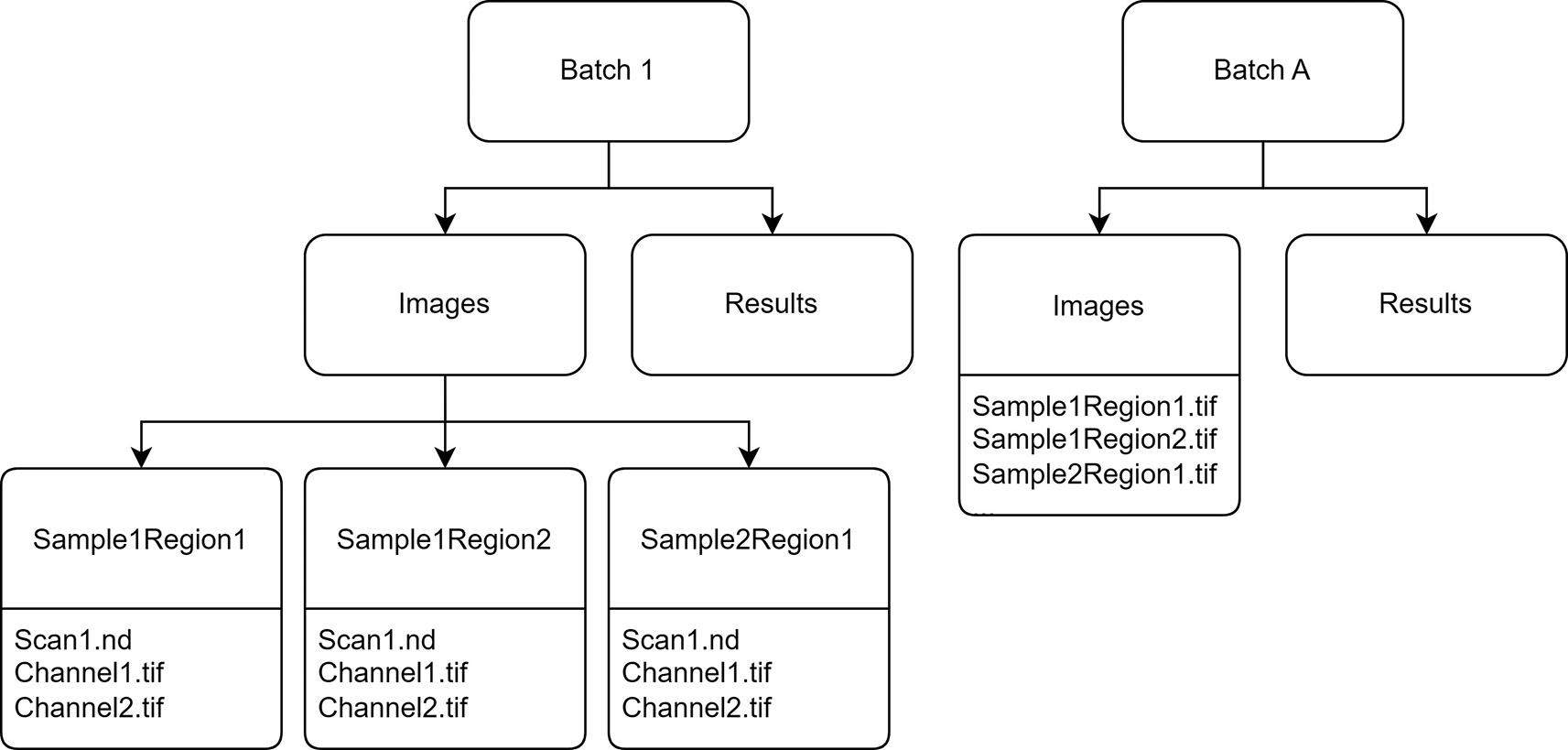
To run, the toolset requires an Image folder containing the experiment and an initially empty Results folder. Two types of Image folder and naming organization are possible (Figure 1): either a master folder contains one subfolder per image (such as is required for .nd files where a given subfolder contains the .nd file and one .tif image per channel), or a single folder contains all the images. In the former case, the name of each subfolder needs to include: the identifier of the sample (such as unique identifying code) and the name of the region analyzed (such as “ACC” for anterior cingulate cortex or “PC” for parietal cortex). In the latter case, the name of the image must include this information.

Figure 1. Examples of suitable folder organization and naming.

The toolset was run on a workstation with an Intel^® Core™ i9-10900 CPU @ 2.80GHz, 128 GB of RAM, and Windows 10 64-bit.

COverlap comprises four macros that can be individually triggered by four action buttons. Each macro performs a specific step (Figure 2):

Figure 2. Complete COverlap workflow.

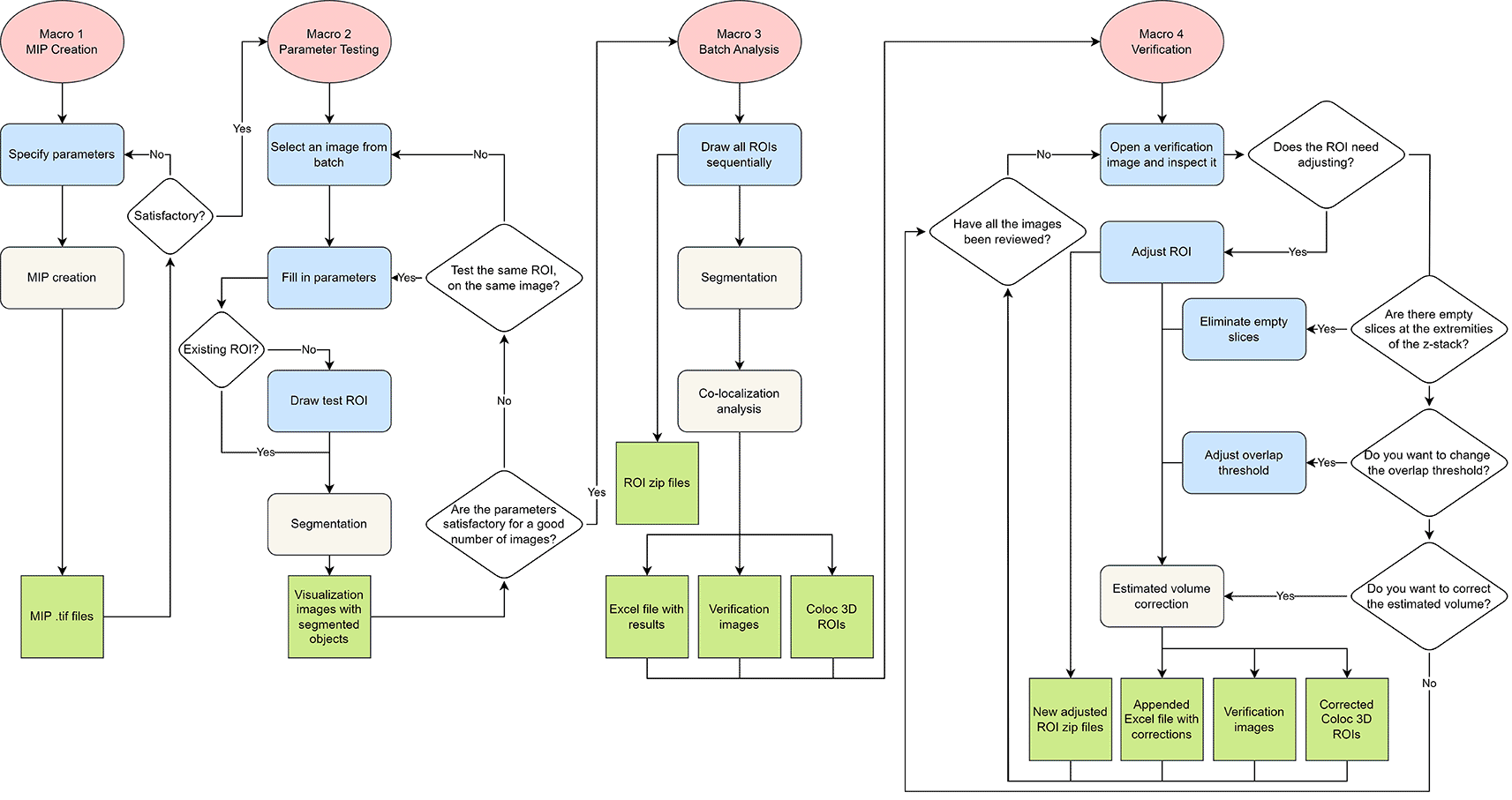
Red bubbles: Macros. Blue: Manual steps. Grey: automated steps. Green: output elements.

The first macro of this toolset allows for the creation of an MIP for each image of the batch and saves it as a TIFF file in the corresponding image folder.

The MIPs generated in this preliminary step will be used as a visualization tool, both as a support for drawing the ROI during the parameter-testing phase (Macro 2) and the batch analysis (Macro 3), and for the creation of verification images on which the positions of co-localization events found during the batch analysis are displayed on the MIP, making it easy for users to locate them and appreciate their distribution (Macros 4).

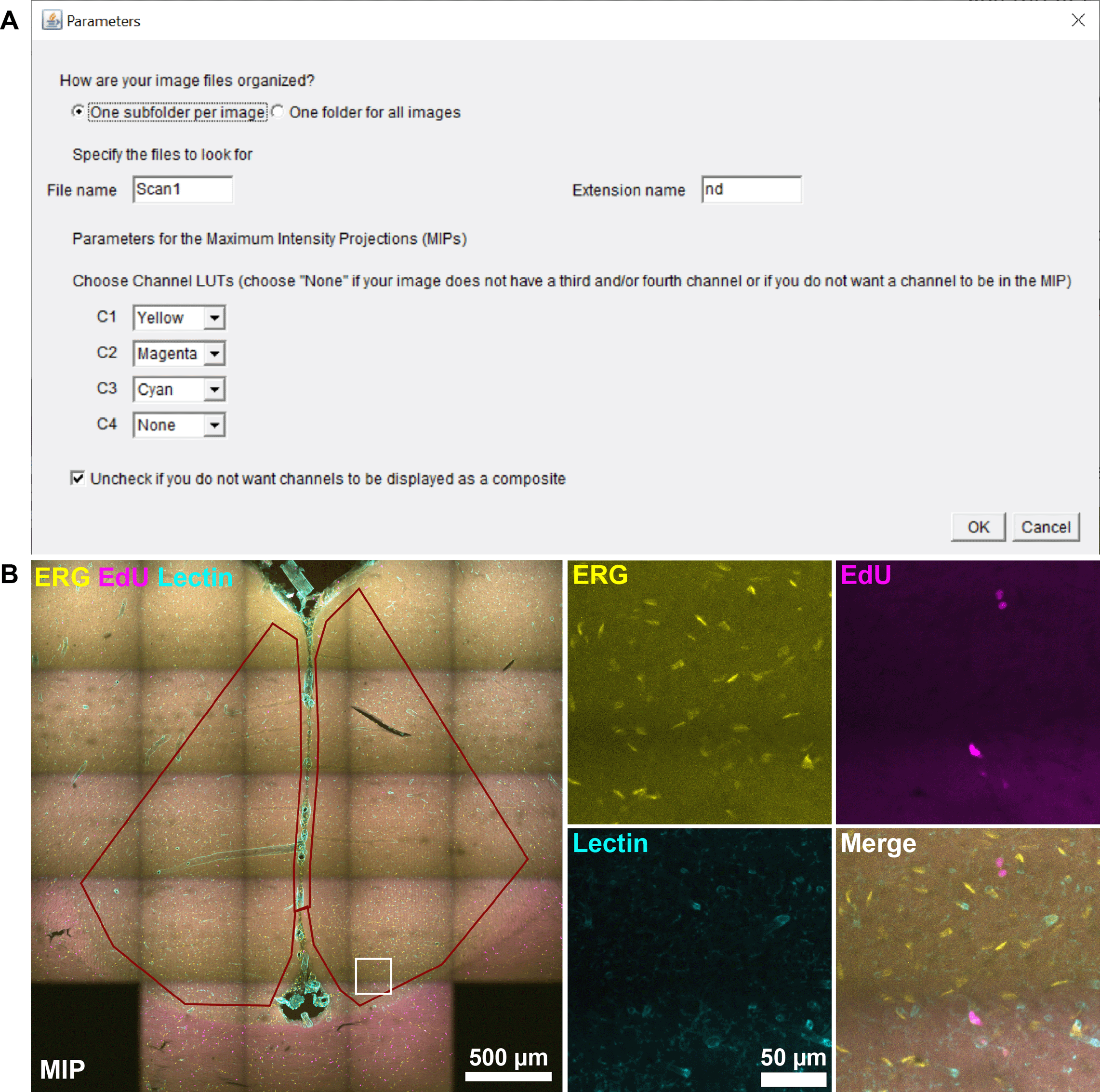
A click on the “1” icon of the toolset launches the first macro, and users are invited to specify the folder organization of their images (Figure 1), a substring (sequence of characters) contained in the file name of all the images, and the extension of images that need to be retrieved from the folder. If no substring is specified, then all images of the specified extension type are processed. Users can then pick a different Lookup Table (LUT) for each channel they want to be part of the MIP or the option “None” for non-existing channels or channels they do not wish to project. An option for disabling the automatic display of all channels as a composite image is also available.

The second macro allows users to test various segmentation parameters (filtering, object minimum size, background subtraction, and threshold) on small portions of images.

Users are invited to point to their Images and Results folders and to specify the names of their target markers and the channel on which they are located. Users can also indicate the names of one and up to two ROIs. These region names should be included in the names of the images that contain them for the macro to properly use their respective associated parameters. If incorrectly spelled or no regions are specified, the left-column parameters will be used for all images. The point of this feature is to allow for region-specific thresholds to be chosen, for example, in cases where different brain regions whose contents are systematically different were imaged. Notably, the current implementation of the macro only works with one ROI per image.

As done previously, users must also provide a substring contained in all image file names, as well as their extension, for the macro to retrieve them in the image folder. These parameters can be saved for retrieval during the subsequent steps of the toolset or later use of the macro.

The macro then displays a list of paths on which users are invited to click to open an MIP from the batch. Once an MIP is opened, users fill in various segmentation parameters in the interface. After they select a representative portion of the image and add it to the ROI Manager, the macro will crop the original image around this test ROI and perform the segmentation test for both channels automatically.

The segmentation of the two nuclear markers of interest performed by this second macro consists of the same steps as those that will be performed during the batch analysis with the third macro (Figure 3). Both macros duplicate the working channels and close the original image to preserve its integrity. Each subsequent step of the segmentation is sequentially performed on each duplicated channel.

Figure 3. Object-segmentation workflow.

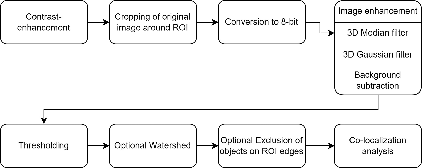
Contrast enhancement is first performed on each slice of the z-stack, by way of the histogram stretching method (also called normalization, Process > Enhance contrast… in ImageJ), where pixel values of the image are recalculated so their range is linearly “stretched” to be equal to the maximum range for the data type (for example 0-65535 for 16-bit images), with 0.35% pixels allowed to become saturated (to prevent a few outlying pixels from causing the histogram-stretch to not work as intended). Each channel is then cropped around the ROI previously drawn by the user and subsequently converted to an 8-bit image by linearly scaling from min-max to 0-255, where min and max values are the “Display range” in Image > Show Info or the values displayed in the Image > Adjust > Brightness > Contrast tool.

Image enhancement processes are then applied: first, denoising is achieved using a 3D median filter¹⁸ (Plugins > 3D Suite > Filters > 3D Fast Filters) chosen for its edge-preserving qualities, followed by a 3D Gaussian filter (Process > Filters > Gaussian Blur 3D) to further smooth images. 3D filtering takes into account possible voxel anisotropy: if the voxels are non-cubic, the ratio between the x and y parameters and the z parameters should approximate that of the ratio between the x and y dimensions and the z dimension of the voxel. The rolling ball background subtraction is then performed (Process > Background subtraction) on each slice of the stack in order to get rid of uneven background fluorescence, which would prevent a global thresholding from working. As a rule of thumb, the selected radius of the rolling ball must be at least as large as the radius of the largest object to be detected in the image. Setting parameters to 0 for any of the enhancement processes will result in the macro skipping this particular step.

The images are then ready for segmentation. The images are processed using the users’ numerical threshold parameter for each channel and the Plugins > 3D Suite > Segmentation > 3D Simple Segmentation. The plugin is based on connected-component analysis, which clusters voxels above an intensity threshold based on their connectivity (here, using an algorithm where all 26 neighboring voxels, including diagonally, are considered connected) and assigns a value to each cluster (see Chapters 2 and 9 of Ref. 20). This method generates a labeled image where each segmented object is attributed to a gray level and has the advantage of including a minimum size filter that allows the exclusion of smaller particles that are out of the nucleus of interest size range.

Users have the option to apply a watershed algorithm to segmented images using the Plugins > 3D Suite > Segmentation > 3D Watershed Split plugin, chosen for its ability to split merged objects based on the local maxima of their Euclidean distance map (i.e., the farthest points from the boundaries of objects, corresponding to their centers). The watershed radius should be approximately the radius of the objects of interest in a given channel.

Users can optionally exclude objects that touch the edges of the ROI. For this, the labeled image is binarized (objects appear in white and the background in black), and the ROI is drawn in white as a two-pixel line on each slice of the z-stack. The image is then converted back into a labeled image, where the ROI and any object that it touches are labeled as a single object. The largest object in the image is then removed, thereby removing the drawn ROI and the touching objects. Users should be advised that this algorithm cannot function properly if the image contains a very large object that comprises more voxels than the object composed of the ROI and the objects it touches. However, this is unlikely in the case of images used for nuclei segmentation and co-localization. The ROI should also be drawn in a single line, so that its border is continuous: any hollow in the ROI created with the “Alt” key will result in the object exclusion feature not functioning. As this feature is mostly useful to avoid detecting spurious co-localization events on the edge of the ROI due to partially segmented objects, we also advise users to disable it during Macro 2 to save processing time.

The result of this automated segmentation test can then be visualized. For both channels, users can compare the original (contrast-enhanced) image, the enhanced (filtered/background subtracted) image, and the composite visualization image displaying the test ROI and the outline of the segmented nuclei (green LUT) on the original image (red LUT). Users can browse the z-stack and toggle the segmentation outline on and off to assess whether their marker of interest has been properly segmented using the chosen parameters.

Parameters can be repeatedly tested until a suitable set is reached without having to reopen the image each time, and users can switch to another image without exiting the macro to test these parameters on a different sample. When a given set of parameters is deemed applicable to the majority of images in the batch, a “Save parameters” box can be ticked before running the test, which generates a file that the third macro retrieves to fill in the graphical user interface (GUI) for parameters automatically. Users can then proceed to batch analysis using the Macro 3.

The third macro performs segmentation and co-localization analysis on the entire batch of images. Users indicate the batch folder containing all the images and MIPs generated with Macro 1 (or image subfolders where each holds an original image and its MIP), as well as a separate output folder (which may contain saved parameters from Macro 2) to store the results, ROIs, and verification images.

Users are prompted to check the targets, channels, and regions parameters that are retrieved from the file saved in Macro 2 and modify them if needed. Similarly, the macro retrieves the segmentation parameters saved in Macro 2 to fill the GUI, and users can check and modify them as needed. If the “Save parameters” box is ticked, the previously saved parameters are overwritten. In any case, when the analysis is started, all the detection parameters used for the batch, as well as the date and time of processing, are saved in the Results folder.

The macro then opens each MIP in turn, and users are prompted to draw one ROI per image, on which the analysis will be performed. As this process may take a long time, proportional to the number of images in the batch and the complexity of the region to be drawn, we advise that users plan ahead and divide their batch into several smaller, more manageable batches if they have a limited amount of time to dedicate to ROI drawing. If users wish to use the edge-exclusion option (see Macro 2), the ROI edges must be continuous (as opposed to having holes drawn in with the Alt key). Users can skip drawing an ROI on images that they do not wish to analyze, as the macro will later ignore images without a matching ROI. Once all the images have been read, the segmentation and co-localization analyses are performed. Alternatively, users can place an already created set of ROIs in the Results folder and uncheck the “Ask for ROI” option in the segmentation GUI. Each ROI must be named after its corresponding image (after the following example “ImageName_ROI.zip”). This technique can also be used in cases where ROIs have already been drawn once, and the analysis must be run again.

For each image, both channels are first segmented using the same process as that described for Macro 2, before the object-based co-localization analysis is performed.

Our method initially defines objects that possess overlapping voxels as co-localized and allows the setting of a minimum percentage of voxels (relative to the total number of voxels in the object, i.e., a minimum volume overlap ratio) that need to be overlapping to be considered as co-localization. For two labeled images obtained from two channels A and B, the MultiColoc plugin of the 3D Suite computes all co-localizations (i.e., all intersections of voxels) between every possible A-B pair of objects. The macro then selects only pairs of objects for which, for at least one of the two objects, the volume overlap ratio meets or exceeds the overlap threshold set in the parameters. If the threshold is set at 50%, only pairs comprising at least one object for which at least 50% of its total volume overlaps the other object will be retained. Notably, this method allows multiple co-localizations to be preserved for a single object.

Depending on the hardware specifications, especially for large batches and/or large images, the analysis can take a long time. The progress is displayed in the Log window (image being processed/total number of images), while the macro runs in the background (images are not displayed). Each time an image is processed, the Results folder is updated, such that if the macro is interrupted before its completion, the results for images that have been successfully analyzed are not lost. Specifically, for each image analyzed, the results table is updated, a.zip file containing a set with the 3D ROIs of each co-localizing object is saved, and two types of verification images are created.

The results table summarizes, for each analyzed sample: the parent folder it belonged to (which can be named after a relevant group or batch name), the sample’s name, its target region, its number of z-slices, the area of the drawn ROI, the total area and the volume analyzed, the number of segmented objects for channels A and B, the number of objects A co-localizing in B, the number of objects B co-localizing in A for a given overlap threshold, and the date and time of processing.

The first type of verification image is a .jpg image based on the MIP from Macro 1, which displays the outline of the analyzed ROI, as well as enlarged outlines around the found co-localization events. Its purpose is to facilitate the localization of these events for users, who can also obtain a general idea of their distribution in the analyzed ROI. The other type of verification image is a .tif image comprised of a z-stack with four binary channels: two (red and green) channels corresponding to each marker segmentation, one (blue) to the co-localization events detected by the macro, and one (grey) to the overlap of objects that were excluded by the co-localization threshold. The first three channels of this image are displayed as a composite, such that any detected co-localization will conveniently appear in white, through the superposition of the three red, green, and blue LUTs. The purpose of this image is to enable users to verify both the segmentation and the co-localization analysis in the analyzed volume: major segmentation problems (such as an inappropriate threshold resulting in noisy segmentation) and spurious co-localization events should be apparent in this image. Users can also review the initially hidden fourth channel to assess the appropriateness of their overlap threshold.

In addition to these verification images, a set of 3D ROIs for co-localizing objects is also saved for each image containing co-localization events. Using the 3D Manager plugin,¹⁸ users can perform additional measurements on co-localized objects, such as intensity measurements on the original image and measurement of volume or other geometric properties.

Once the analysis is completed, a message is displayed in the Log window, and the text file containing the detection parameters is appended with the date and time of completion of the analysis. Users can then proceed to the review step at any time they deem convenient.

The fourth macro allows users to review their analyzed images and perform corrections, such as trimming of the ROI (e.g., to exclude an air bubble trapped in the mounting medium between the slide and coverslip), reslicing of the z-stack (to exclude out-of-focus slices), changing the overlap threshold for co-localizations, or correcting the volume estimation.

After inputting their Images and Results folders, users indicate the name of the targets and their respective channels, as well as the original overlap threshold with which the images have been analyzed. The macro then retrieves and displays the list of verification images from the Results folder. Users are invited to open a composite image from the list to review it. They can open the corresponding MIP visualization image at the same time to check where the detected co-localization events are located, but must close it before the next step. When they are ready to perform corrections, users click on the OK button and are presented with a list of corrections that may be applied to the image. If they confirm that they wish to perform corrections, the “Correction Options” GUI is displayed.

Users can perform several actions:

Once the options are set, the macro performs all the above-mentioned corrections. Objects are quantified again with these new parameters, from the corrected composite image directly, without having to reopen the original image, and co-localizations are analyzed again for these objects. An important feature of this correction step is that it corrects the estimated analyzed volume.

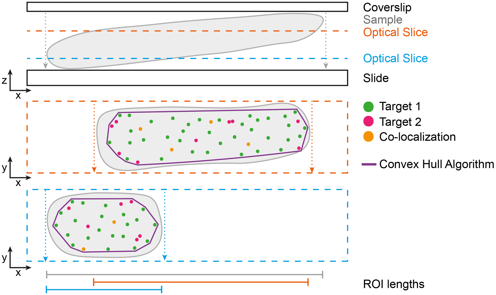
While the initially calculated volume corresponds to the area of the ROI multiplied by the number of z-slices multiplied by the size of the z-step, this algorithm wraps, for each slice, a convex hull selection around all detected cells regardless of the channel and uses the sum of these selections’ areas multiplied by the size of the z-step in place of the original formula. This allows users to base the analysis only on the volume that has objects in it and is especially useful when the biological sample is not perfectly flat on the microscope slide and does not fill the totality of the ROI in the first and/or last few slices of the z-stack (Figure 4). Users can ignore this option and rely on the “cookie-cutter” ROI-based volume estimation, which is also provided and considers the new ROI shape and the new number of slices (e.g., in the case of a very sparse labeling or if the exact same ROI is being used for all images).

Figure 4. Correction of estimated volume with Convex Hull Algorithm.

Following corrections, new files are saved in the Results folder, containing the mention “Adjusted” in their name: the new ROI if it has been modified, the new visualization images (Composite and MIP) showing the corrected analysis, and the new set of 3D ROIs for co-localizing events that users can later review or use for measurements.

One advantage of this review step is that while the whole process may take time for large batches of images, users do not have to review all images at once and can use the macro any number of times to review parts of the batch. Because the macro appends, retrieves, and displays the original Results file, users can easily know where they left off the previous time and continue their review work at a later time.

In the parameters GUI of Macro 1 (Figure 5A), we indicated that our Image folder contained one subfolder per image, in which a file always named “Scan1.nd” was stored with its three corresponding .tif channel images. An example of a resulting MIP with the three chosen LUTs is shown in Figure 5B. Although only the first two channels (ERG and EdU labeling) were used for quantification, we chose to include the third channel with the Lectin staining on MIPs to facilitate the visualization of the vascular network.

Figure 5. A. Macro 1 graphical user interface. B. Example of maximum intensity projection (MIP) with zoomed in inserts. Red outline: anterior cingulate cortex (ACC) region of interest.

We used Macro 2 to determine the best set of parameters for the segmentation of ERG⁺ and EdU⁺ nuclei. Due to slight batch-dependent differences in background fluorescence, we chose different thresholds for a given batch but kept the minimum size, filtering, and background subtraction parameters consistent across batches (Figure 6A). This was made possible by the fact that our experimental conditions were evenly distributed among batches, and we advise against such a choice if it introduces a potential bias in the experimental results. Here, we assume that despite our efforts to perform the staining and imaging protocol in an identical manner for all batches, a number of slight variations may have occurred that could explain this difference, such as the percentage of error during pipetting, temperature variations during heat-induced antibody retrieval, or duration of mounting medium curing (7-10 days before the first day of imaging for one batch).

Figure 6. A. Segmentation graphical user interface for Macros 2 and 3. B. Output of a test on a small region of interest (cyan outline): Top panels: ERG channel, Bottom panels: EdU (5-ethynyl-2’-deoxyuridine) channel. Left: original, contrast-enhanced image. Middle: Original, contrast-enhanced image with Red Lookup Table and yellow outlines of segmented nuclei. Right: Filtered image with cyan outlines of segmented nuclei.

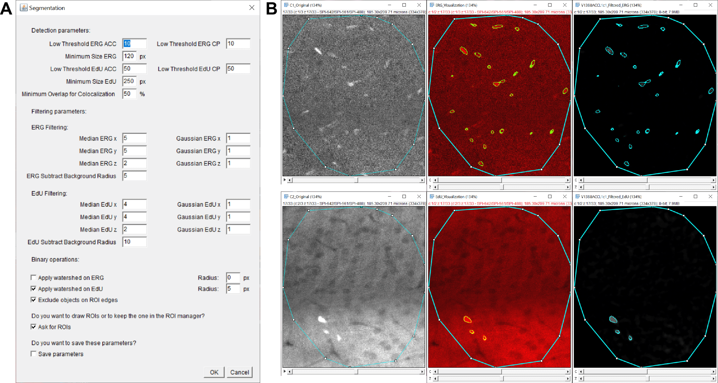
We performed multiple rounds of testing on multiple images. For each image, various small representative ROIs were selected to test the segmentation parameters. The output of such a test is presented in Figure 6B: toggling the outline on and off and examining the filtered image output helped us determine the optimal parameters for the segmentation of our targets. When we found the best compromise for the majority of images in a given batch, we ticked the “Save parameters” box before starting the last test. The parameters selected for each batch are listed in Table 1.

We launched Macro 3 separately for each batch with their set of segmentation parameters determined with Macro 2 (Table 1) and with an overlap threshold set at 30%, chosen to reliably exclude false positives while still accounting for size and shape differences between EdU and ERG labeling.

We drew an ROI for only 359 of the 360 images because the MIP inspection revealed a problem with the tile-stitching of one image in Batch 3. The processing time, number of images, and data size for each batch are listed in Table 2. One GB of images required a mean 3:35 minutes of processing time, which corresponded to a mean of 11:19 min per image.

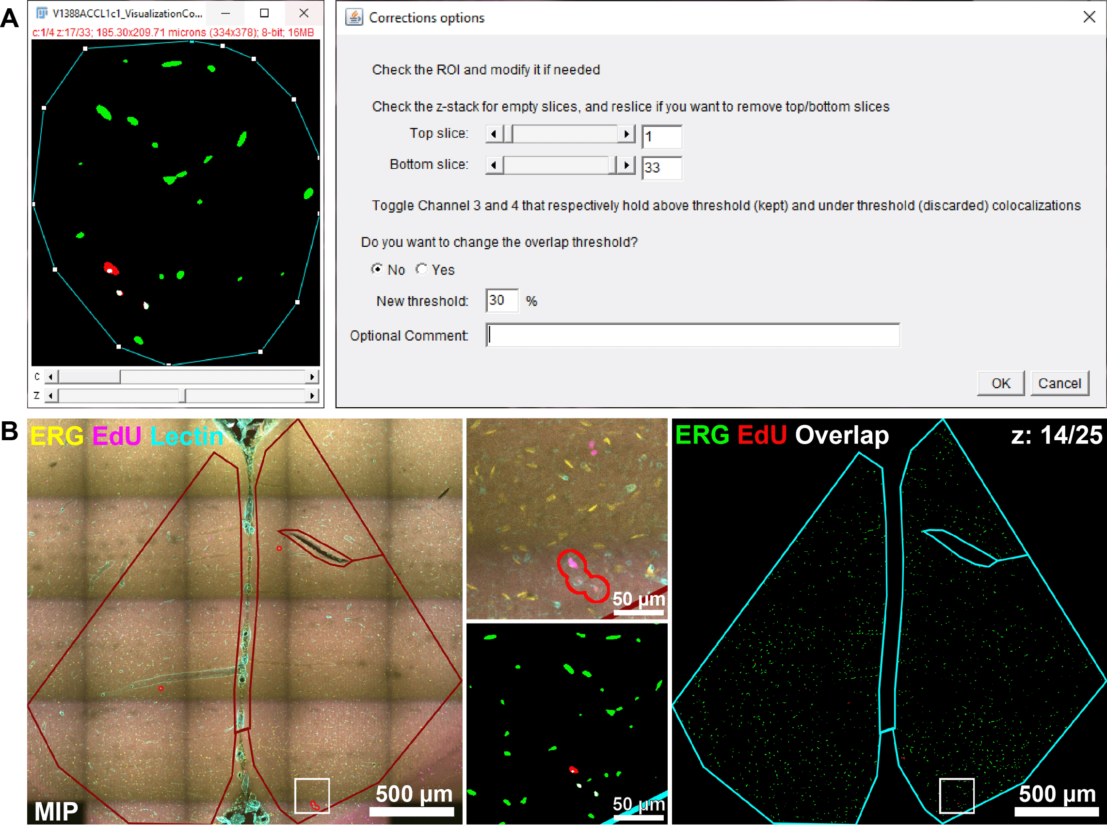
All 359 verification images were inspected using the Macro 4. We filled the corrections GUI (Figure 7A) for each image requiring adjustments and chose to perform volume estimate correction (Figure 4) for all images regardless. Example of adjusted verification images (.jpg MIP and .tif composite files) produced by this correction step are shown in Figure 7B.

Figure 7. A. Left: Example of composite image opened by Macro 4 (a sample region of interest (ROI) was used for better visibility, ERG objects appear in green, EdU (5-ethynyl-2’-deoxyuridine) in red and co-localizing objects in white). Right: Corrections graphical user interface. B. Example of adjusted verification images after corrections have been performed. Left: maximum intensity projection (MIP) with red overlay showing modified ROI excluding a tear and location of co-localization events (inset: middle top). Right: Z-slice 14 of the composite verification image (inset: middle bottom).

The “Comment” section was particularly useful to report problems with images. We also systematically used it to describe the reason for a ROI modification. We tried to be consistent in our qualification of identical issues or justifications across images in order to classify them after the batch was fully reviewed (e.g. using “Sparse” to describe sparsely labeled ERG or “Removed corpus callosum” for a ROI modification).

DISCARDED IMAGES

The review revealed that two animals presented a complete absence of EdU labeling, indicative of injection issues since other animals in the same histology batch were normally labeled; all acquired images for these animals (four of the ACC and two of the PC each) were excluded from further analysis.

Of the 347 remaining images, 15, all from the PC region, were also discarded upon first inspection: one because of an error in which the same slice had been acquired twice, and the others because the tissue was too damaged and/or improperly mounted to produce accurate segmentation. In general, tissue from the PC was more damaged than that from the ACC.

Inspection of the appended results file revealed that due to the rather weak labeling of ERG, some of the remaining 332 images were annotated as “Sparsely labeled” in the optional comments section. We chose to set a density of object/mm³ threshold to exclude sparsely labeled images in a reproducible way and excluded 31 (23 CP, 9 ACC) images for which the density of labeled ERG cells was less than 3500 ERG objects per mm³.

CORRECTIONS PERFORMED

Of the 301 z-stacks left, 292 (97%) were resliced to exclude out-of-focus optical slices, indicating that the range of the z-stack acquisition was consistently too generous. This type of information is crucial for planning future experiments, in which care will be taken to acquire a shorter range in z.

Eighteen (≈6%) ROIs were adjusted to exclude air bubbles in the mounting medium (6), damaged or torn tissue (5, as illustrated in Figure 7B), or part of the corpus callosum that was unduly encompassed in the initial ROI drawing (7).

The co-localization overlap threshold was deemed satisfactory and maintained at 30% for all images.

EXPERIMENTAL RESULTS

For the two targets (number of ERG⁺ and number of EdU⁺ objects) and for the two possible types of co-localization events (number of ERG⁺ objects in EdU⁺ objects and number of EdU⁺ objects in ERG⁺ objects), we calculated the density of objects per mm³ of analyzed tissue (using the corrected volume estimate) for all valid slices, and averaged them to obtain a mean density per region for each animal. The results are shown in Figure 8.

Figure 8. Mean densities of objects per mm³ with standard error of the mean (SEM).

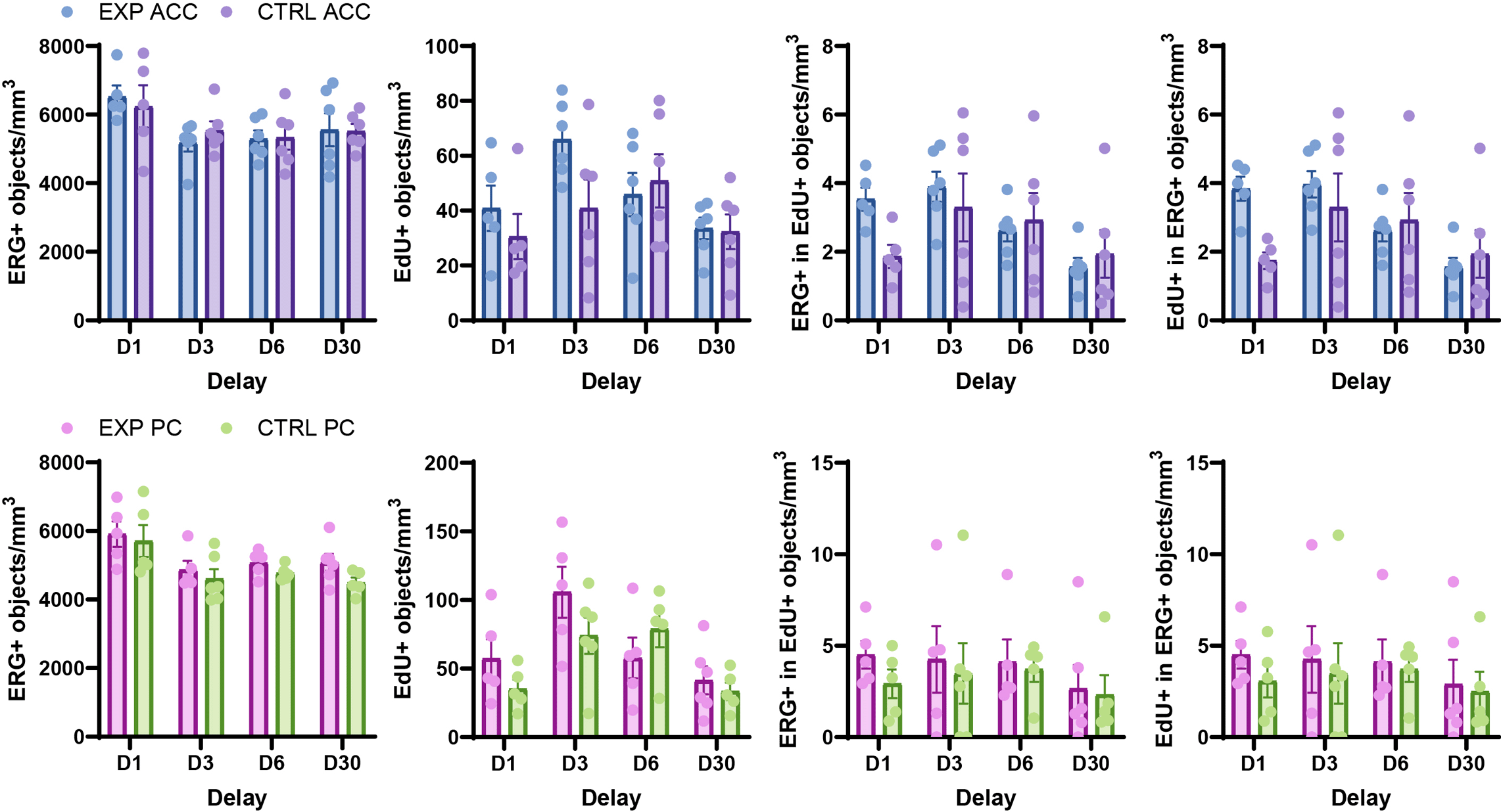
Individual data points correspond to mean of slices per animal.

We performed Šídák’s multiple comparison test using GraphPad Prism for each brain region to determine whether, for each post-encoding delay, the experimental and control groups had significantly different object densities. None of the comparisons revealed significant differences between the groups (Table 3).

Normalization is a critical choice and may not be appropriate for all types of analysis. First, care must be taken that the relative intensity distribution is nearly identical for all images in the experiment. Second, it should be noted that while normalization may be convenient for visualization and segmentation purposes, it represents a loss of information (in our case, 0.35% of pixels are allowed to become saturated) and may alter results if further processing steps are based on absolute gray values.²⁶ Here, normalization facilitates nuclei segmentation despite varying illumination along the depth of the samples.²⁶ Likewise, users may not want to downscale images acquired with a higher bit-depth to 8-bit, as this also results in a loss of information. In our case, however, it allows us to work with lighter images, which speeds up processing without compromising segmentation quality. Additionally, the narrower range of gray values simplifies the testing and selection of a suitable intensity threshold.

We have included three steps in the workflow that are classically used to enhance images for the purpose of segmentation (see Chapter 3 in Ref. 20): two spatial nonlinear (median) and linear (Gaussian) filters to denoise images and smooth out irrelevant details, and Fiji’s rolling ball algorithm (based on Ref. 27) to eliminate background fluorescence. Taking advantage of the parameter GUI, a step can be omitted by setting its parameter to zero, making it possible to apply each step alone or in combination with one or two other steps. Although users can choose the parameters, the order in which the steps are performed cannot be modified without modifying the code. If this workflow proves ineffective in enhancing more complex images, users may want to consider alternative denoising techniques (reviewed in Refs. 28, 29) and illumination correction methods.^30–32

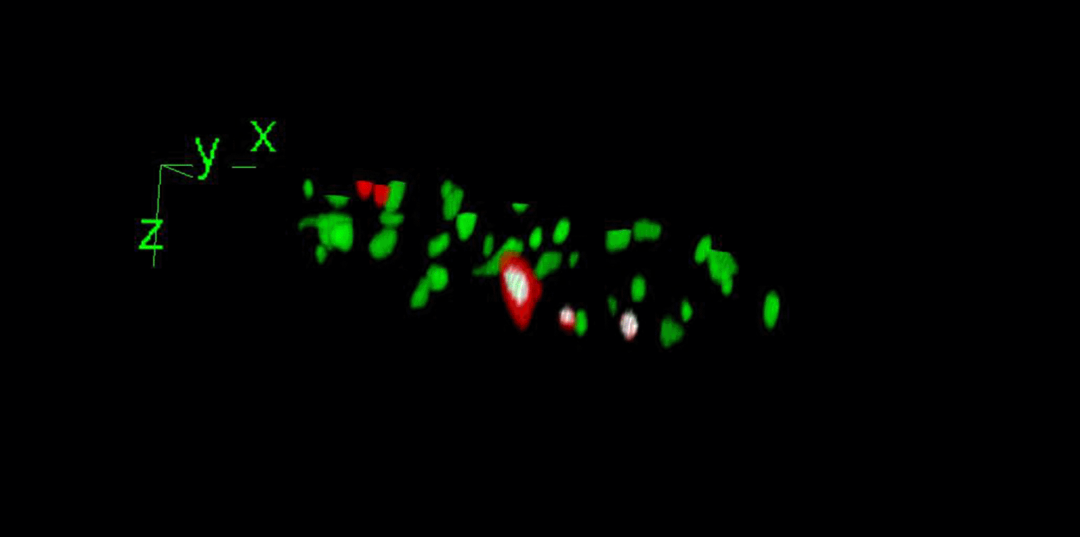
Nucleus segmentation in 3D presents a much greater challenge than in 2D³³ but provides several advantages. In contrast to segmenting the MIP of the stack, it prevents false positives that can occur in the co-localization analysis when nuclei are located atop one another in z. Compared to limiting the analysis to a single z-plane, it maximizes the quantity of information analyzed by allowing the segmentation of at least two layers of nuclei along the z-axis (Figure 9). This has the added benefit of preserving the three-dimensional geometry of the nuclei and better describing their spatial relationship in situ.

Figure 9. 3D representation of segmented objects and co-localization from the example region of interest in Figure 7A.

We implemented the 3D Simple Segmentation of the 3D Suite,¹⁸ which consists of thresholding pre-processed images, performing connected component analysis, and filtering out objects by size. When necessary, the 3D watershed algorithm of the 3D Suite was applied to separate the touching objects. To avoid excluding touching nuclei that the watershed algorithm might not have separated, we solely implemented the minimum size and excluded the maximum-size filter. We employed a numerical threshold, as suggested by the plugin’s interface, which we empirically found performed satisfactorily on our preprocessed images. Nevertheless, if an automatic threshold is preferred, minor modifications to the code would permit it, because the plugin can operate on a previously obtained binary mask by setting the threshold at 1. If both numerical and automatic thresholds fail to consistently extract objects, users can attempt to implement the iterative thresholding algorithm of the 3D Suite.¹⁸

Our segmentation method would certainly exhibit limitations for densely packed or overlapping nuclei that represent a difficult segmentation case, even for more advanced tools.³³ In our experiment, EdU⁺ nuclei were sparsely distributed and often appeared in doublets which the watershed algorithm was able to properly split when they were touching. In addition, the endothelial nuclei were sufficiently spaced to be segmented satisfactorily. However, owing to the elongated shape of ERG⁺ objects, we abstained from applying the watershed algorithm to prevent their over-segmentation. We recognize that our result for the density of ERG⁺ objects might be slightly underestimated because some touching objects were counted as a single entity. While this does not hinder the co-localization analysis, it makes the density of EdU⁺ in ERG⁺ objects a more dependable indicator than the density of ERG⁺ in EdU⁺, because co-localizing EdU⁺ objects are still expected to exceed the overlap threshold, while touching ERG⁺ objects counted as a single object may not.

Deep learning (DL) methods have revolutionized the field of bioimage analysis and are quickly becoming the gold standard for classification, denoising or segmentation.³⁴ For the latter, some DL solutions are now accessible to biologists with limited computational skills (listed in recent reviews^33,35,36), but most are difficult to set up and use, especially for 3D segmentation.³³ Moreover, user-friendly platforms such as deepImageJ³⁷ rely on pretrained models, which are currently not widely available in 3D. Training new models from scratch requires extensive computing power in the case of 3D data as well as large annotated datasets that are time-consuming and difficult to produce.³⁸ While we wager that these challenges will soon be overcome given the rapid expansion of the field, we chose to use a classical method that does not have such heavy hardware or annotation requirements.