Keywords
RNA-Seq, pathway enrichment, R package, topology, KEGG, Reactome, scRNA-seq
This article is included in the Bioconductor gateway.
A common outcome of analysing RNA-Seq data is the detection of biological pathways with significantly altered activity between the conditions under investigation. Whilst many strategies test for over-representation of genes, showing changed expression within pre-defined gene-sets, these analyses typically do not account for gene-gene interactions encoded by pathway topologies, and are not able to directly predict the directional change of pathway activity. To address these issues we have developed sSNAPPY,now available as an R/Bioconductor package, which leverages pathway topology information to compute pathway perturbation scores and predict the direction of change across a set of pathways.
Here, we demonstrate the use of sSNAPPY by applying the method to public scRNA-seq data, derived from ovarian cancer patient tissues collected before and after chemotherapy. Not only were we able to predict the direction of pathway perturbations discussed in the original study, but sSNAPPY was also able to detect significant changes of other biological processes, yielding far greater insight into the response to treatment. sSNAPPY represents a novel pathway analysis strategy that takes into consideration pathway topology to predict impacted biology pathways, both within related samples and across treatment groups. In addition to not relying on differentially expressed genes, the method and associated R package offers important flexibility and provides powerful visualisation tools.
R version: R version 4.3.3 (2024-02-29)
Bioconductor version: 3.18
Package: 1.6.1
RNA-Seq, pathway enrichment, R package, topology, KEGG, Reactome, scRNA-seq
Using pathway enrichment analysis to gain biological insights from gene expression data is a pivotal step in the analysis and interpretation of RNA-seq data, for which numerous methods have been developed (reviewed in1,2). Many existing methods tend to view pathways simply as a collection of gene names, as seen in those relying on the detection of differentially expressed genes and applying over-representation analysis (ORA) strategies, with alternative methods being those scoring all genes using functional class scoring (FCS), such as in Gene Set Enrichment Analysis (GSEA),3 arguably the most widely-used approach. However, databases such as the Kyoto Encyclopaedia of Genes and Genomes (KEGG)4 and WikiPathways5 capture not only which genes are implicated in a certain biological process but also their interactions, activating or inhibitory roles, and their relative importance within the pathway, all of which are overlooked in ORA- and FCS-based approaches.
To fully utilise this additional information, the latest generation of pathway analysis approaches include many which are topology-based such as SPIA,6 DEGraph,7 NetGSA8 and PRS,9 as well as others which explicitly model inter-gene correlations.10 Despite differences in the null hypotheses tested across these approaches, overall, they have demonstrated enhanced sensitivity and specificity due to their abilities to take gene-gene interconnections into account.11,12 Nevertheless, most topology-based methods focus only on comparing the activity of pathways between two treatment groups and cannot be used to score individual samples (Figure 1). However, in heterogeneous data where more than one factor may be influencing observations,13 incorporating scoring within paired samples may be desirable and may be able to reveal more nuanced insights. To address this gap, we present a Single-Sample directioNAl Pathway Perturbation analYsis methodology called sSNAPPY, available as an R/Bioconductor package. This article defines how sSNAPPY computes changes in gene expression within paired samples and propagates this through gene-set topologies, to predict the perturbation in pathway activities within paired samples, before providing summarised results across an entire dataset (Figure 1). The practical usage of the sSNAPPY R/Bioconductor package is illustrated through the analysis of a public scRNA-seq dataset using a pseudo-bulk approach, demonstrating its applicability to both bulk RNA-Seq and scRNA-Seq datasets.
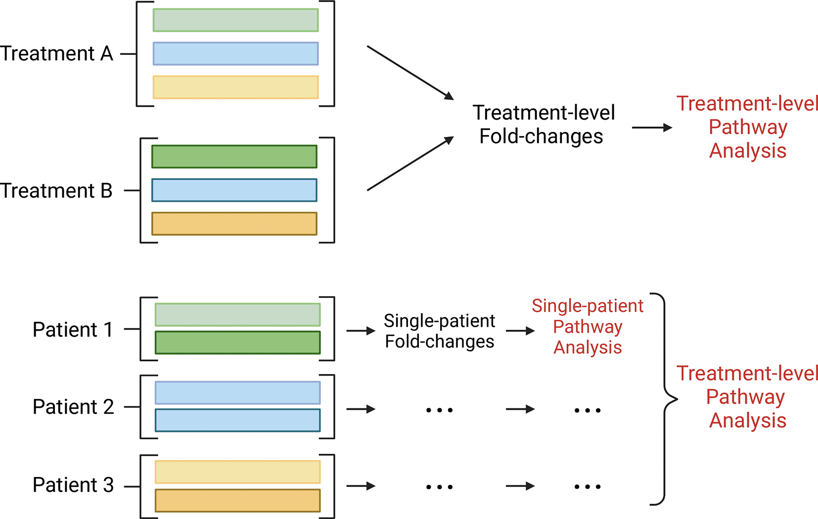
Instead of being limited to treatment-level analyses, sSNAPPY allows the detection of pathway perturbation within individual samples by using sample-specific estimates of fold-change instead of experiment-wide estimates. (Created with BioRender.com).
sSNAPPY is an R package that has been reviewed and published on the open-source bioinformatics software platform Bioconductor with all source code available via GitHub. The methodology itself is topology-based, designed to compute directional, single-sample, pathway perturbation scores for gene expression datasets with matched-pair, or nested designs (e.g. samples collected before and after treatment). Common examples of such designs may include treated vs control samples within cell-line passages, or across multiple treatments applied to tissue samples from within a specific donor. This allows for the detection of pathway perturbations within all samples from a treatment group, but also within individual samples, with sSNAPPY providing results in the form of pathway perturbation scores 1) for each set of paired samples, and 2) across all paired samples within an experimental grouping. The only data required to run sSNAPPY, is a log-transformed expression matrix (e.g. logCPM) with matching sample metadata describing treatment groups and the nested structure. It is assumed that all pre-processing has been performed beforehand, such as the exclusion of low-signal genes or normalisation to minimise technical artefacts like GC-bias.
The first step performed by sSNAPPY, is to estimate sample-specific log fold-change () across all genes , for each treatment , and within each set of nested replicates , by subtracting expression estimates for the baseline samples from those in treatment group . It should also be noted that sSNAPPY is applicable to any number of treatment/condition levels and that sample numbers within each treatment group are not required to be balanced.
It is well known that in RNA-seq data, genes with lower expression tend to have greater variability in signal and more broadly spread estimates of change.14 As such, we utilise a gene-level weighting strategy to down-weight fold-change estimates for low-abundance genes prior to passing these estimates to sSNAPPY. Gene-level weights are obtained in a treatment-agnostic manner by fitting a loess curve through the relationship between observed gene-level variance () and average signal ()(Figure 2), and taking the inverse of the loess-predicted variance as the weight , where is the predicted value from the loess curve and the constant ensures . We then use these globally-weighted estimates of log fold-change () in the calculation of all subsequent pathway perturbation scores.
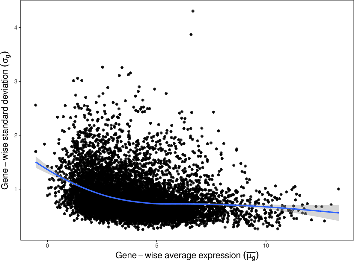
The relationship between standard deviations and expression levels is modelled by a loess fit. Whilst standard deviations are shown for the purposes of visualisation, gene-level weights are calculated using variances at this stage of the sSNAPPY algorithm.
sSNAPPY extends the topology-based scoring algorithm initially proposed in SPIA6 which propagates fold-change estimates from genes considered as differentially expressed through pathway topologies, to compute a perturbation score for each pathway. In contrast to SPIA, which relies on a defined set of differentially expressed genes, sSNAPPY uses fold-change estimates from all detected genes. By modifying the algorithm to incorporate single-sample, weighted estimates of fold-change, we are able to numerically represent changes in a pathway within a given sample, and subsequently model these across all samples within a treatment group. Thus, we define the single-sample perturbation score () for a given pathway and treatment for a set of nested samples :
and:• represents the set of genes in pathway , such that
• is the gene-, treatment- and sample-specific perturbation score for pathway
• is the weighted log fold-change of gene as described above
• is the subset of containing only the genes directly upstream of gene , and not including gene
• is the pair-wise gene-gene interactions6 encoded by the topology matrix for genes and
• is the number of downstream genes from any gene
• is the accumulated pathway perturbation score for pathway in treatment within sample across all genes in the pathway
To scale single-sample pathway perturbation scores () so they are comparable across pathways, and to test for significance of individual scores, null distributions of perturbation scores for each pathway are generated through a sample permutation strategy, which retains any existing correlation structures between genes within a pathway. During permutation, all sample labels are randomly shuffled and permuted pseudo-pairs formed from the re-shuffled labels. Single-sample fold-changes are then calculated for each pseudo-pair of permuted samples while the rest of the scoring algorithm remains unchanged. The median and median absolute deviation (MAD) are calculated from the set of permuted perturbation scores within each pathway and used to normalise the raw perturbation scores to robust -scores, i.e. .
All possible permuted pseudo-pairs are sampled unless otherwise specified, such that in an experiment with total samples, the maximum number of unique permuted pairs is . Permutation p-values are calculated for each value, indicating the approximate significance of pathway perturbation at the single-sample level. Relying on symmetry around zero, these are derived by assessing the proportion of permuted scores with absolute values as extreme, or more extreme, than the absolute value of test perturbation score within each pathway.15 Since the smallest achievable permutation p-value is 1/, accurate estimation of small p-value requires a large number of permutations that is only feasible in data with a large sample size. As a guideline, GSEA recommends a minimum of 7 samples in each treatment group for utilizing their phenotype permutation approach,16 and under sSNAPPY this would yield = 182 unique permuted pseudo-pairs and minimal permutation p-values of at each individual sample and pathway-level.
Apart from assessing whether a pathway’s activity is changed significantly within an individual sample, an important question may be the detection of changes in pathway activity across all samples within a treatment. This can be performed by modelling values using regression models and incorporating Smyth’s moderated t-statistic17 as implemented in limma.18 The single-sample nature of sSNAPPY’s pathway perturbation scores is particularly helpful for datasets with complex experimental designs or known confounding factors as these can also be incorporated into the final regression models.
The Bioconductor package graphite19 provides functions that can be used to retrieve pathway topologies from a database and convert topology information to adjacency matrices. To streamline this process, we have implemented a convenience function, where users only need to provide the name of the desired database and species to retrieve all topology information in the format required by the scoring algorithm with the correct type of gene identifiers (i.e. EntrezID). Importantly, we noted that graphite19 retrieves topology matrices in varied orientations from different databases; in KEGG pathways, columns represent downstream relationships, whereas in Reactome and WikiPathway, columns indicate upstream regulation. However, this discrepancy is not taken account of in the runSPIA() function of graphite. We resolve the issue by transposing the topology matrices retrieved from the Reactome and WikiPathway as part of our convenience function.
The set of additional required packages for this workflow can be installed using
pkg <- c(
  "tidyverse", "patchwork", "kableExtra", "AnnotationHub", "edgeR", "here",
  "pander", "colorspace", "SPIA", "fgsea"
)
BiocManager::install(pkg, update = FALSE, force = FALSE, ask = FALSE)
Once installed, the complete set of packages can be loaded into the session.
library(sSNAPPY)
library(tidyverse)
library(magrittr)
library(patchwork)
library(kableExtra)
library(AnnotationHub)
library(edgeR)
library(pander)
library(colorspace)
library(SPIA)
library(fgsea)
Retrieving pathway topology information from a chosen database is the next key step required during preparation for running sSNAPPY, and this is the only step requiring internet access. If running on an HPC cluster where internet access may be restricted, this step can be performed separately with topologies saved by the user as an RDS object. Using the Reactome database20 in this workflow, the retrieved topology information will be stored as a list where each element corresponds to a pathway and the numbers in the matrices encode gene-gene interactions.
gsTopology <- retrieve_topology(database = "reactome", species = "hsapiens")
In addition to downloading topology matrices for all pathways, it is also possible to provide a restricted set of keywords for a targeted analysis. For example, passing the argument keyword = c("metabolism", "estrogen") would only return the subset of pathways which match either of these keywords. Multiple databases are also able to be searched by passing a vector of database names to the database argument.
To demonstrate the application of sSNAPPY, we used pre-processed counts from a publicly available scRNA-seq dataset, retrieved from Gene Expression Omnibus (GEO) with accession code GSE165897. This dataset consists of 11 high-grade serous ovarian cancer (HGSOC) patient samples taken before and after chemotherapy.21 sSNAPPY was used to re-analyse data from the epithelial cells as they were the primary focus of the original study. Since sSNAPPY was designed primarily for bulk RNA-seq data, counts from epithelial cells within the same samples were first summed into pseudo-bulk profiles, giving rise to a total of 22 samples. We considered a gene detectable if we observed >1.5 counts per million in 11 of the 22 samples, ideally representing all samples from a complete treatment group. 11,101 (33.8%) of the 32,847 annotated genes passed this selection criteria and were included for downstream analyses. Conditional quantile normalisation22 was then applied to mitigate potential biases introduced by gene length and GC content. The normalised logCPM matrix of the processed dataset and sample metadata can be downloaded from here.
To begin running the sSNAPPY workflow, we first load our expression matrix and define our sample-level metadata. Importantly, the row names of the expression matrix must be specified as EntrezGene IDs, for compatibility with pathway databases. Genes without EntrezGene IDs were excluded during pre-processing, leaving 10,098 genes in the example expression matrix. The treatment column within our metadata is expected to be a factor, with the reference level interpreted as the control treatment.
readr::local_edition(1)
logCPM <- read_tsv(here::here("data/logCPM.tsv")) %>%
  column_to_rownames("entrezid")
sample_meta <- read_tsv(here::here("data/sample_meta.tsv"), col_types = "cfccncnc")
head(sample_meta)

## # A tibble: 6 × 8
##   sample         treatment  patient_id anatomical_location Age Stage PFI CRS
##   <chr>           <fct>       <chr>      <chr>             <dbl> <chr> <dbl> <chr>
## 1 EOC372_treat … treatmen … EOC372     Peritoneum         68 IIIC    460 1
## 2 EOC372_post- … post-NACT  EOC372     Peritoneum         68 IIIC    460 1
## 3 EOC443_post- … post-NACT  EOC443     Omentum            54 IVA     177 3
## 4 EOC443_treat … treatmen … EOC443     Omentum            54 IVA     177 3
## 5 EOC540_treat … treatmen … EOC540     Omentum            62 IIIC    126 2
## 6 EOC540_post- … post-NACT  EOC540     Omentum            62 IIIC    126 2
To compute the single-sample fold-changes (i.e. logFC) required for the set of perturbation scores, samples must be ‘matched pairs’ or nested, as discussed earlier, and treatments performed within each patient represents the nesting structure in this dataset. The factor (patient_id) defining the nested structure is passed to weight_ss_fc() using the groupBy parameter.
weightedFC <- weight_ss_fc(
  as.matrix (logCPM), metadata = sample_meta,
  sampleColumn = "sample", groupBy = "patient_id", treatColumn = "treatment"
)
glimpse (weightedFC)
The output of weight_ss_fc() is a list where one element is the matrix of weighted single-sample fold-changes (), with rows corresponding to genes and columns to samples, and the other element is the vector of gene-wise weights () used to calculate the weighted log fold-change (). By default, the string ENTREZID: is added to all row names of the matrix to be compatible with the format Reactome pathway topologies are retrieved in.
The matrix of values is then passed to pathway topologies to compute gene-wise perturbation scores for all genes within a pathway, before being summed into a single score for each pathway. The function raw_gene_pert() returns an initial list, with each element containing the gene-level perturbation scores for a given pathway. These matrices are also able to be used during downstream analysis to identify which genes play the most significant roles in each pathway, as demonstrated in later sections. Pathway-level perturbation scores () are then returned as a data.frame containing sample and gene-set names after calling pathway_pert(). Pathways with zero perturbation scores across all genes and samples are automatically dropped at this step. In addition, pathways with aggregated pathway-level scores of zero in all samples will also be dropped by default, unless otherwise specified through the drop parameter of the pathway_pert() function.
genePertScore <- raw_gene_pert(weightedFC$weighted_logFC, gsTopology)
ssPertScore <- pathway_pert(genePertScore, weightedFC$weighted_logFC)
ssPertScore %>%
    split(f = .$gs_name) %>%
    keep(~all(. != 0)) %>%
    length()
## [1] 1093
head (ssPertScore)
##             sample         score                           gs_name
## 1 EOC372_post-NACT -2.292688e-04 reactome. Interleukin-6 signaling
## 2 EOC443_post-NACT -2.447003e-04 reactome. Interleukin-6 signaling
## 3 EOC540_post-NACT -1.848758e-04 reactome. Interleukin-6 signaling
## 4   EOC3_post-NACT -1.229489e-04 reactome. Interleukin-6 signaling
## 5  EOC87_post-NACT  3.427132e-05 reactome. Interleukin-6 signaling
## 6 EOC136_post-NACT  2.822155e-04 reactome. Interleukin-6 signaling
The range of values obtained from the complete set of pathways will vary greatly, due to the variability in topology structures. To determine the significance of individual scores and transform scores to ensure they are comparable across pathways, sSNAPPY utilises a sample-permutation strategy to estimate the null distributions of perturbation scores and derive scores. Since sample labels will be permuted randomly to put samples into pseudo-pairs, sample metadata is not required by the generate_permuted_scores function. All possible random pairs between samples will be sampled unless otherwise specified. In this example dataset with a total of 22 samples, the full set of 462 (i.e. ) permuted scores will be computed for each pathway.
permutedScore <- generate_permuted_scores(
  as.matrix (logCPM),
  gsTopology = gsTopology[names(genePertScore)],
  weight = weightedFC$weight
)
Apart from pathways whose permuted perturbation scores are consistently zero, and which will be dropped by default, the empirical distributions of remaining pathways are expected to be approximately normally distributed with mean , but with the scale of distributions heavily impacted by both the number of genes within each pathway and the overall topology. To demonstrate this, we randomly selected 6 pathways to demonstrate their quantile-quantile (q-q) plot and visualised the distributions of their permuted perturbation scores as boxplots (Figure 3).
set.seed(123)
random_pathways <- permutedScore %>%
  keep(~all(. != 0)) %>%
  .[sample(seq_along(.), 6)] %>%
  as.data.frame() %>%
  pivot_longer(
    cols = everything(), names_to = "gs_name", values_to = "score"
  ) %>%
  mutate(
    gs_name = str_replace_all(gs_name, "\\.", " "),
    gs_name = str_remove_all(gs_name, "reactome ")
  )
p1 <- random_pathways %>%
  ggplot(aes (sample = score, colour = gs_name)) +
  stat_qq() +
  stat_qq_line(colour = "black") +
  facet_wrap(~str_wrap(gs_name, width = 25), scales= "free") +
  labs(y = "Permuted Perturbation Score", x = "Theoretical Quantiles") +
  theme_bw() +
  theme(
    legend.position = "none",
    text = element_text(size = 14),
    strip.text = element_text(size = 16))
p2 <- random_pathways %>%
  ggplot(aes (gs_name, score, fill = gs_name)) +
  geom_boxplot() +
  scale_x_discrete(labels = function(x) str_wrap(x, width = 10)) +
  scale_fill_discrete(name = "Gene-set Name") +
  labs(x = "Pathway", y = "Permuted Perturbation Score") +
  theme_bw() +
  theme(
    legend.position = "none",
    axis.title = element_text(size = 16),
    axis.text = element_text(size = 14)
  )
(p1/p2) +
  plot_annotation(tag_levels = "A") +
  plot_layout(heights = c(0.6, 0.4))
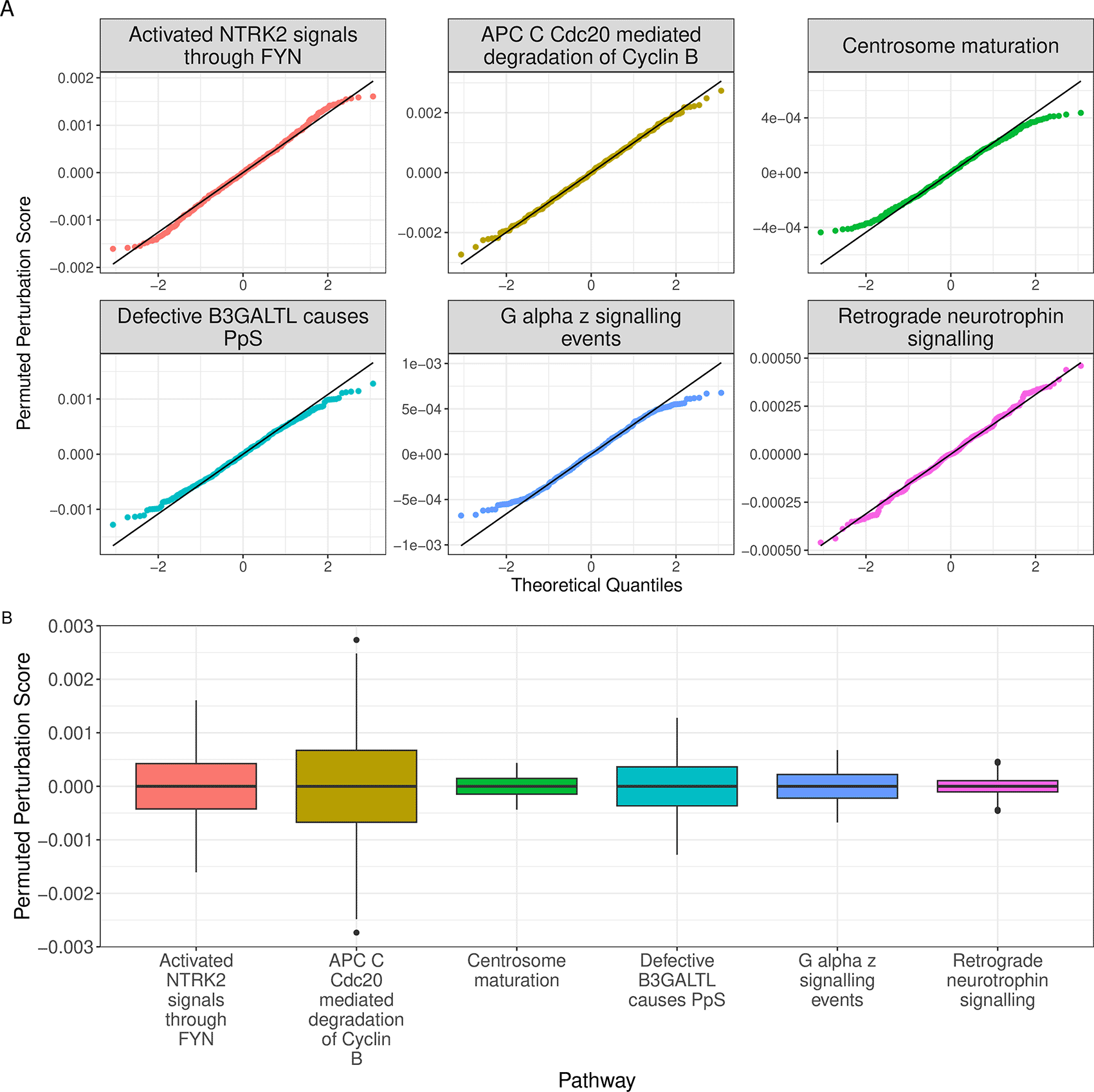
All sampled empirical distributions are approximately normally distributed with a mean of zero.
The distributions obtained from label permutations are then used to convert each pathway-level score into the robust -score using the function normalise_by_permu(). Two-sided p-values for individual scores are computed based on how extreme test scores are in comparison to permuted scores for each pathway and corrected for multiple testing using any of the available methods, returning the FDR-adjusted values by default. In our example data, no pathways would be considered as significantly perturbed at the single-sample level using an FDR adjustment with = 0.05.
normalisedScores <- normalise_by_permu(permutedScore, ssPertScore,
                                       sortBy = "pvalue")
head (normalisedScores)

##               MAD MEDIAN
## 2306 0.0006067519      0
## 2525 0.0002909911      0
## 5869 0.0001652241      0
## 5871 0.0001652241      0
## 5872 0.0001652241      0
## 7721 0.0275863198      0
##                                                           gs_name
## 2306 reactome.Golgi Cisternae Pericentriolar Stack Reorganization
## 2525       reactome.DNA Damage/Telomere Stress Induced Senescence
## 5869                        reactome.Defective CHST6 causes MCDC1
## 5871           reactome.Defective ST3GAL3 causes MCT12 and EIEE15
## 5872       reactome.Defective B4GALT1 causes B4GALT1-CDG (CDG-2d)
## 7721                        reactome.Mitochondrial protein import
##                sample         score   robustZ      pvalue adjPvalue
## 2306 EOC153_post-NACT -0.0013632057 -2.246727 0.004329004 1.0000000
## 2525 EOC153_post-NACT  0.0006149637  2.113342 0.004329004 1.0000000
## 5869 EOC349_post-NACT -0.0003304944 -2.000279 0.004329004 0.9993248
## 5871 EOC349_post-NACT -0.0003304944 -2.000279 0.004329004 0.9993248
## 5872 EOC349_post-NACT -0.0003304944 -2.000279 0.004329004 0.9993248
## 7721 EOC443_post-NACT -0.0598366717 -2.169070 0.004329004 0.9471861
A key question of interest in our example dataset is to identify which biological processes were impacted by chemotherapy across the entire group of patients. Using the sample-level output obtained above, we can explore this by applying t-tests or regression models across all samples. In order to minimise spurious results, Smyth’s moderated t-statistics17 can be applied across the complete dataset, with a constant variance assumed across all pathways, given that we are using Z-scores. To perform this analysis, values were converted to a matrix and standard limma methodologies were used. For our use case here, where only one treatment group is present, no design matrix is required, and a simple t-test is appropriate.
z_matrix <- normalisedScores %>%
  dplyr::select (robustZ, gs_name, sample) %>%
  pivot_wider(names_from = "sample", values_from = "robustZ") %>%
  column_to_rownames("gs_name") %>%
  as.matrix()
z_fits <- z_matrix %>%
  lmFit(design = rep(1, ncol(.))) %>%
  eBayes()
top_table <- topTable(z_fits, number = Inf) %>%
  as_tibble(rownames = "gs_name")
sigPathway <- dplyr::filter (top_table, adj.P.Val < 0.05)
121 out of the 1094 tested Reactome pathways have an FDR < 0.05 in the moderated t-test, and were considered to be significantly perturbed at the group level. Table 1 presents the top 10 significantly inhibited and activated pathways, along with their predicted direction of change.
table 1 <- sigPathway %>%
  mutate(
    Direction = ifelse (logFC < 0, "Inhibited", "Activated"),
    gs_name = str_remove_all(gs_name, "reactome.")
  ) %>%
  split(f = .$Direction) %>%
  lapply (dplyr::slice, 1:10) %>%
  bind_rows() %>%
  dplyr::select(
    Pathway = gs_name, Change = logFC, P.Value, FDR = adj.P.Val, Direction
  )
For enrichment analysis in the original study,21 unsupervised clustering was performed on all cells labelled as cancer cells. Clusters were then annotated manually by performing pathway enrichment testing on cluster marker genes. Two clusters, associated with proliferative DNA repair signatures and stress-related markers, contained significantly higher numbers of post-chemotherapy cells than pre-treatment ones.21 The representative pathways enriched in the stress-associated cluster were IL6-mediated signaling events, TNF signaling pathway, and cellular responses to stress, and the other post-chemotherapy cell dominated cluster in the original study was enriched for pathways associated with cell proliferation and DNA repair, such as the Cell cycle, DNA repair, Homology directed repair (HDR) through homologous recombination, and the Fanconi anaemia pathway.
Whilst the published enrichment analysis was performed using ConsensusPathDB,23 in order to use pathway topologies we chose the Reactome set of pathways.20 sSNAPPY not only detected many significant perturbed pathways that are highly concordant with the pathways reported to be enriched in the original study but also includes an expected direction of change in activity. For example, the DNT repair pathway SUMOylation of DNA damage response and repair proteins pathway was predicted to be significantly inhibited by chemotherapy. The single-sample nature of the sSNAPPY output also provides great flexibility: apart from considering all treated samples as biological replicates, users may elect to perform an analysis incorporating other phenotypic traits which may impact a patient’s responses to chemotherapy, such as disease stages or tumour grades. To perform this step using the moderated t-statistic strategy and extend the above analysis, an appropriate design matrix is the only additional requirement for model-fitting, or alternatively, samples may be subset as may be appropriate.
A valuable feature of sSNAPPY is the provision of several visualisation functions to assist in the presentation and interpretation of results. Biological pathways are not independent of each other with many genes playing a role across multiple pathways, and as such, viewing pathway analysis results as a network can be a powerful way to intuitively summarise the results and facilitate interpretation of the underlying biology. The plot_gs_network() function allows users to easily convert a list of relevant biological pathways to a network where edges between pathway nodes represent overlapping genes. Defined by the colorBy parameter, pathway nodes can be coloured by either the predicted direction of change or by significance levels (Figure 4). The returned plot is a ggplot224 object, meaning that components of the plotting theme and other parameters can be customized as for any other ggplot2 objects.
In the following example, we’ll inspect the 10 most significantly inhibited and 10 most significantly activated pathways, which involved four steps to prepare the data: 1) rename the logFC column to reflect the true meaning of the value and, 2) create a categorical variable with the pathway status, 3) transform p-values for simpler visualisation and 4) obtain a subset of pathways to visualise.
sigPathway <- sigPathway %>%
  dplyr::rename(Z = logFC) %>%
  mutate(
    status = ifelse(Z > 0, "Activated", "Inhibited"),
    status = as.factor(status),
    '-log10(p)' = -log10(P.Value)
  ) %>%
  split(f = .$status) %>%
  lapply(dplyr::slice, 1:10) %>%
  bind_rows()
# Plot the network structure
set.seed(150)
p1 <- plot_gs_network(
  normalisedScores = sigPathway, gsTopology = gsTopology, colorBy = "status",
  gsNameSize = 3
) +
  scale_colour_manual(values = c("red", "blue", "grey30")) +
  theme_void() +
  theme(
    legend.text = element_text(size = 10),
    legend.position = "inside",
    legend.position.inside = c(0.95, 0.95)
  )
set.seed(150)
p2 <- plot_gs_network(
  normalisedScores = sigPathway,
  gsTopology = gsTopology,
  colorBy= "-log10(p)",
  gsNameSize = 3,
  gsLegTitle = expression(paste(-log[10], "p"))
) +
  scale_colour_viridis_c() +
  theme_void() +
  theme(
    legend.text = element_text(size = 8),
    legend.title = element_text(size = 10),
    legend.position = "inside",
    legend.position.inside = c(0.95, 0.95)
  )
p1/p2 + plot_annotation(tag_levels = "A")
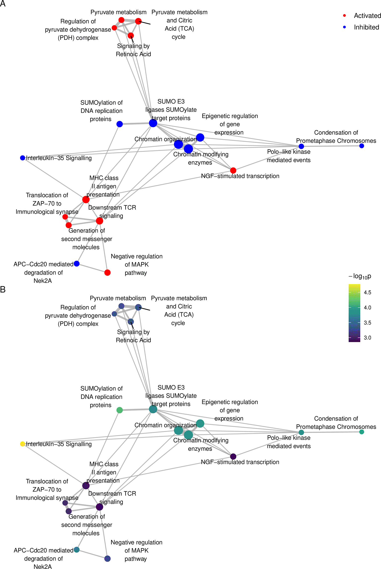
Each node represents a significantly perturbed Reactome pathway, with nodes coloured by (A) predicted direction of change and (B) -log10(p). The 10 most significantly inhibited and 10 most significantly activated pathways are shown.
An advantage of visualising pathway analysis results using network structures is that it allows the identification of highly connected pathways (Figure 4). To summarise related pathways and further enable interpretation, we can apply community detection25 to group related pathways into ‘communities’. sSNAPPY’s plot_community() function is a “one-stop shop” for applying a community detection algorithm of the user’s choice to the network structure and annotating identified communities by the most common pathway category, denoting the main biological processes perturbed in that community. The most recent categories for both KEGG and Reactome databases were curated from their respective website (KEGG website & Reactome website) and included as parts of sSNAPPY. Analyses involving other pathway databases may require user-provided pathway categories. When the information about pathway categorisations is available, annotation of pathway communities is automatically completed. In the current dataset, the Louvain method was applied to the network of biological pathways and revealed five primary communities: 1) Adaptive Immune System; 2) Cell Cycle, Mitotic; 3) Chromatin modifying enzymes & Epigenetic regulation of gene expression; 4) Post-translational protein modification and 5) The citric acid (TCA) cycle and respiratory electron transport (Figure 5). The largest community formed was the Adaptive Immune System pathway, indicating a clear immune-signalling aspect to these results.
load(system.file("extdata", "gsAnnotation_df_reactome.rda", package = "sSNAPPY"))
set.seed(199)
plot_community(
    normalisedScores = sigPathway,
    gsTopology = gsTopology,
    gsAnnotation = gsAnnotation_df_reactome,
    colorBy = "status",
    lb_size = 3
) +
  scale_colour_manual(values = c("red", "blue")) +
  scale_fill_viridis_d() +
  scale_x_continuous(expand = expansion(0.2)) +
  scale_y_continuous(expand = expansion(0.2)) +
  guides (fill = "none") +
  theme_void() +
  theme(
      legend.position = "inside",
      legend.position.inside = c(0.9, 0.1)
  )
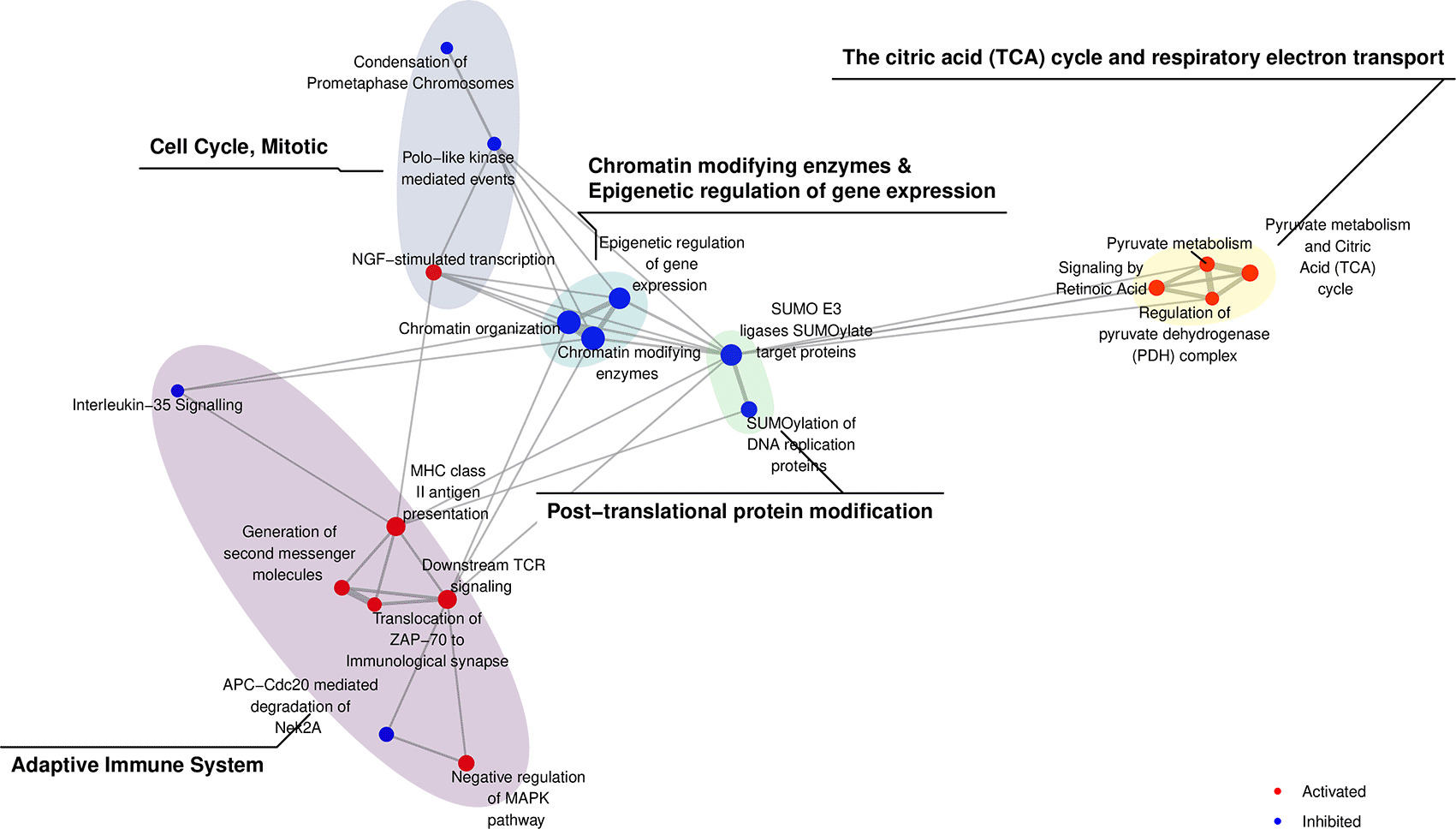
The Louvain algorithm was applied to detect community structures, revealing biological processes associated with highly ranked pathways. The top 20 which were the most perturbed by chemotherapy are shown.
A key advantage of sSNAPPY is that it does not require the prior identification of differentially expressed genes, as this is a common challenge faced within clinical datasets. However, knowing which genes are implicated in the perturbation of pathways, particularly those which influence multiple pathways, can provide valuable insights for hypothesis generation and the underlying biological mechanisms. Therefore, sSNAPPY provides another visualisation feature called plot_gs2gene, which enables the inclusion of select genes from each pathway using network structures. Users can provide a vector of fold-change estimates to visualise genes within pathways, showing their estimated change in expression. As pathways often include hundreds of genes, it is recommended to filter for genes most likely to be playing a significant role. In this example dataset, only genes within the top 500 when ranking by the magnitude of the mean ssFC were included (Figure 6). An alternative strategy will be to select genes based on test-statistics, however, this decision is up to the individual researcher.
meanFC <- rowMeans(weightedFC$weighted_logFC)/weightedFC$weight
top500 <- rank(1/abs (meanFC)) <= 500
Since Reactome pathway topologies were retrieved using EntrezIDs, users can provide a data.frame mapping EntrezIDs to their chosen identifiers, such as gene names, through the mapEntrezID parameter, in order to make the visualisations more informative. A data.frame converting EntrezIDs to Ensembl gene names was derived from the Ensembl Release 10126 and has been made available as part of the package and serves as a helpful template for future mapping operations by users.
load(system.file("extdata", "entrez2name.rda", package = "sSNAPPY"))
head(entrez2name)

## # A tibble: 6 × 2
##   entrezid           mapTo
##   <chr>              <chr>
## 1 ENTREZID:84771     DDX11L1
## 2 ENTREZID:727856    DDX11L1/DDX11L9/DDX11L10
## 3 ENTREZID:100287102 DDX11L1
## 4 ENTREZID:100287596 DDX11L1/DDX11L9
## 5 ENTREZID:102725121 DDX11L1
## 6 ENTREZID:653635    WASH7P

set.seed(195)
plot_gs2gene(
  normalisedScores = sigPathway,
  gsTopology = gsTopology,
  colorGsBy = "status",
  mapEntrezID = entrez2name,
  geneFC = meanFC[top500],
  layout = "kk",
  edgeAlpha = 1,
  gsNodeSize = 5,
  geneNodeSize = 3,
  gsNameSize = 4,
  geneNameSize = 3.5
) +
  scale_colour_gradient2(name = "Mean ssFC", low = "orange", high = "green4") +
  scale_fill_manual(values = c("red", "blue")) +
  theme_void() +
  theme(
    legend.text = element_text(size = 12),
    legend.title = element_text(size = 12)
  )
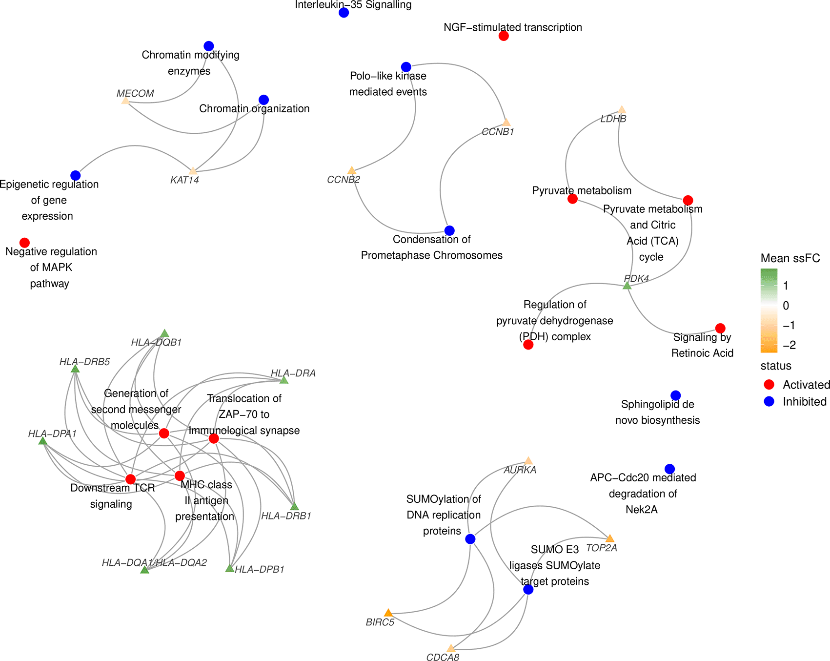
Significantly perturbed Reactome pathways identified among post-chemotherapy samples using sSNAPPY, showing any genes in the top 500 ranked by magnitude of change in expression, and which pathways they are likely contributing to. Only the 10 most significantly inhibited and 10 most significantly activated pathways are shown.
To further investigate a specific pathway and elucidate which are the key genes contributing to the final perturbation score, we can generate a heatmap via plot_gene_contribution() which shows the gene-level perturbation scores for the top-ranked members of a given pathway. This function takes advantage of the plotting capabilities of the pheatmap package,27 and as such, other annotations are also able to be easily included, such as patient response, or which general ranges the pathway-level normalised Z-Scores are in. Inclusion of the Z-Scores enabled the assessment of the level of perturbation predicted in each sample and key genes involved (Figure 7).
path_name <- "SUMOylation of DNA replication proteins"
z_breaks <- round(qnorm(c(0, 0.025, 0.05, 0.25, 0.75, 0.95, 0.975, 1)), 2)
annotation_df <- normalisedScores %>%
  dplyr::filter(str_detect(gs_name, path_name)) %>%
  left_join(dplyr::select(sample_meta, sample, CRS), by = "sample") %>%
  mutate(
    'Z Range' = cut(robustZ, breaks = z_breaks, include.lowest = TRUE),
    sample = str_remove_all(sample, "_post-NACT")
  ) %>%
  dplyr::select(sample, 'Z Range', CRS)
z_levels <- levels (annotation_df$'Z Range')
annotation_col <- list(
  CRS = c("3" = "#4B0055", "2" = "#009B95", "1" = "#FDE333"),
  'Z Range' = setNames(
    colorRampPalette(c("navyblue", "white", "darkred"))(length(z_levels)),
    z_levels
  )
)
mat <- genePertScore %>%
  .[[which (str_detect(names(.), path_name))]] %>%
  set_colnames(str_remove_all(colnames(.), "_post-NACT")) %>%
  .[rownames(.) %in% rownames (weightedFC$weighted_logFC),]
max_pert <- max (abs (range (mat))) * 1.01
plot_gene_contribution(
  genePertMatr = mat,
  color = rev (colorspace::divergex_hcl(100, palette = "RdBu")),
  breaks = seq(-max_pert, max_pert, length.out = 100),
  annotation_df =annotation_df,
  annotation_colors = annotation_col,
  filterBy = "mean",
  mapEntrezID = entrez2name,
  cutree_rows = 2,
  cutree_cols = 2,
  main = paste (path_name, "[REACTOME]")
)
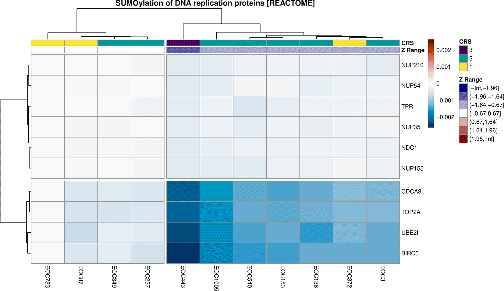
All pathway genes were ranked by average contribution to the perturbation score to select the top 10 genes. Samples were annotated by patient chemotherapy response score (CRS), along with the range for sample-level Z-scores as a guide to sample-specific pathway perturbation. The genes CDCA8, TOP2A, UBE2I, BIRC5 were identified as possible key drivers of inhibition for this pathway.
From this heatmap we can identify four candidate genes which are likely to be making a contribution to the inhibition of the SUMOylation of DNA replication proteins pathway upon chemotherapy, such as CDCA8, TOP2A, UBE2I, BIRC5 (Figure 7). These four genes are all associated with tumour progression and invasiveness and have been studied in the context of ovarian cancer. Both ubiquitin conjugating enzyme E2I (UBE2I) and cell division cycle associated 8 (CDCA8) genes have been identified as oncogenes in numerous cancer types, including ovarian cancer.28,29 Notably, in ovarian cancer, elevated UBE2I expression has been associated with poorer clinical outcomes.30 Similarly, BIRC5 encodes a protein which is also a predictor of inferior ovarian cancer patient outcome.31 Lastly, Topoisomerase II (TOP2A), which encodes DNA topoisomerase, has been identified as a gene that promotes the tumorigenesis of HGSOC tumours.32 Aligning with the report by Chekerov et al.33 that expression of TOP2A in ovarian tumour cells decreases as a response to chemotherapy,33 the median single-sample logFC of TOP2A was negative among the HGSOC post-chemotherapy samples included in this study (Figure 8). The other three selected potential driver genes (CDCA8, UBE2I, and BIRC5) also had negative median single-sample logFC in post-chemotherapy samples (Figure 8). Considering the implication of these four genes in ovarian cancer, decreases in their expression after chemotherapy treatment potentially indicate a favorable response to therapy.
By annotating the heatmap of gene-wise perturbation scores with patient chemotherapy response score (CRS), we also noted that the strongest inhibition of the SUMOylation of DNA replication proteins pathway was in the patient with the highest CRS score of 3 (i.e sample EOC443). CRS is an indicator of the relative length of progression-free survival after chemotherapy, where a score of 3 represents the longest survival. Hence inhibition of the SUMOylation of DNA replication proteins pathway might mediate favorable response to chemotherapy in ovarian cancer patients. We acknowledge that our analysis was limited to a small number of patients, which restricts the generalizability of the results. However, despite this limitation, these findings underscore the strength of sSNAPPY as a valuable tool for hypothesis generation not otherwise possible. Not only can sSNAPPY predict directional pathway perturbations, but it also enables the identification of potential driver genes which are strongly associated with these perturbations.
gene2plot <- entrez2name %>%
  dplyr::filter(mapTo %in% c("CDCA8", "TOP2A", "UBE2I", "BIRC5"))
(weightedFC$weighted_logFC/weightedFC$weight) %>%
  as.data.frame() %>%
  rownames_to_column("entrezid") %>%
  pivot_longer(
    cols = -all_of("entrezid"), names_to = "sample", values_to = "ssFC"
  ) %>%
  inner_join(gene2plot, by = "entrezid") %>%
  ggplot(aes(mapTo, ssFC, fill = mapTo)) +
  geom_boxplot() +
  labs(x = "", fill = "Gene") +
  geom_hline(yintercept = 0, color = "red", linetype = "dashed") +
  theme_bw()
We also performed pathway analysis on this example dataset using three other methods to compare their performance against sSNAPPY. Details on the implementation of those methods and the comparisons performed are available at 10.5281/zenodo.10127829. We initially performed an analysis using SPIA.6 However, SPIA relies on differentially expressed genes and given that only 49 genes were identified in our analysis using conventional differential expression analysis, no pathways were considered to be significant using SPIA. Additionally, we also performed pathway analysis on this example dataset using two non-topological-based approaches: 1) GSEA3 using ranking statistics derived from differential expression analysis and 2) the fast version of rotation gene set testing for linear models (roast)34 fry, neither of which rely on the presence of differentially expressed genes, Importantly, both methods test for signal within genes at either the up-regulated, or down-regulated extremes. Of the 219 gene sets considered associated with down-regulated genes by GSEA, 61 were considered as inhibited using sSNAPPY. Similarly, of the 21 pathways considered as associated with up-regulated genes by GSEA, 5 were considered as activated using sSNAPPY. GSEA produced a further 173 gene-sets not detected by sSNAPPY, whilst sSNAPPY produced an additional 54 pathways of interest.
Analysis using fry yielded 117 pathways associated with down-regulated genes, with sSNAPPY considering 36 of these as inhibited. However, 5 pathways classified as inhibited under fry were considered as activated under sSNAPPY, highlighting that down-regulation of some genes may lead to activation of a pathway, which is vital information not available under fry. Similarly, for the 13 pathways associated with up-regulation under fry, two were considered activated by sSNAPPY, with one considered inhibited. A further 88 pathways were detected as being of interest under fry, without being considered as activated or inhibited by sSNAPPY, with 77 pathways uniquely detected under sSNAPPY.
In conclusion, we have presented and provided a demonstration for the R/Bioconductor package sSNAPPY which offers a novel single-sample pathway perturbation testing approach, tailored for heterogeneous tissue samples where experiments are performed using a matched-pair design. In contrast to many common enrichment methods, sSNAPPY uses pathway topology information to compute perturbation scores which indicate the likely impact on the activity of a pathway, by predicting direction of change and enabling deeper characterisation of biological responses. By applying sSNAPPY to a public scRNA-seq data collected before and after HGSOC patients were subjected to chemotherapy, we demonstrated its ability to detect significant pathway perturbations of various interesting biological processes consistent with, and far beyond what was shown in the original study. Whilst initially conceived for bulk-RNA studies, this demonstration has also provided clear applicability to scRNA datasets when using using pseudo-bulk approaches sSNAPPY addresses the limitations of alternative strategies which fail to account for gene-gene interactions encoded by pathway topologies and are unable to predict the direction of pathway activities, nor the cumulative effect of expression change across multiple genes. In addition, the single-sample nature of the method can be utilised to address the increasing demand for personalised medicine. Through identifying shared and divergent responses between individuals, sSNAPPY can provide valuable insights into the heterogeneous responses across clinical samples. Overall, we believe sSNAPPY represents a valuable addition to the existing body of pathway analysis methods.
WL’s contributions include Conceptualization, Data Curation, Formal Analysis, Investigation, Methodology, Project Administration, Software, Validation, Visualisation, Writing - Original Draft Preparation, and Writing - Review & Editing. VM was involved with Conceptualization, Methodology and Writing - Review & Editing. WDT contributed to Writing - Review & Editing. SMP’s contributions include Conceptualization, Methodology, Project Administration, Software, Supervision, Writing - Original Draft Preparation, and Writing - Review & Editing.
The processed dataset used in this manuscript, along with the code used for data preparation is available at https://doi.org/10.5281/zenodo.10867706.
Raw data was obtained from Gene Expression Omnibus: Longitudinal single-cell RNA-seq data of metastatic ovarian cancer. Accession GSE165897; https://www.ncbi.nlm.nih.gov/geo/query/acc.cgi?acc=GSE165897. 21
• Software available from: https://bioconductor.org/packages/release/bioc/html/sSNAPPY.html
• Source code available from: https://github.com/Wenjun-Liu/sSNAPPY
• Archived source code at time of publication: https://zenodo.org/doi/10.5281/zenodo.8185450
• License: GNU General Public License v3.0 GPL-3
| Views | Downloads | |
|---|---|---|
| F1000Research | - | - |
|
PubMed Central
Data from PMC are received and updated monthly.
|
- | - |
Is the rationale for developing the new software tool clearly explained?
Yes
Is the description of the software tool technically sound?
Yes
Are sufficient details of the code, methods and analysis (if applicable) provided to allow replication of the software development and its use by others?
Yes
Is sufficient information provided to allow interpretation of the expected output datasets and any results generated using the tool?
Yes
Are the conclusions about the tool and its performance adequately supported by the findings presented in the article?
Yes
Competing Interests: No competing interests were disclosed.
Reviewer Expertise: bioinformatics, clinical bioinformatics, transcriptomics, genetics
Is the rationale for developing the new software tool clearly explained?
Partly
Is the description of the software tool technically sound?
Yes
Are sufficient details of the code, methods and analysis (if applicable) provided to allow replication of the software development and its use by others?
Yes
Is sufficient information provided to allow interpretation of the expected output datasets and any results generated using the tool?
Yes
Are the conclusions about the tool and its performance adequately supported by the findings presented in the article?
Yes
References
1. Yang P, Patrick E, Tan SX, Fazakerley DJ, et al.: Direction pathway analysis of large-scale proteomics data reveals novel features of the insulin action pathway.Bioinformatics. 2014; 30 (6): 808-14 PubMed Abstract | Publisher Full TextCompeting Interests: No competing interests were disclosed.
Reviewer Expertise: Statistical Bioinformatics
Alongside their report, reviewers assign a status to the article:
| Invited Reviewers | ||
|---|---|---|
| 1 | 2 | |
|
Version 1 13 Jun 24 |
read | read |
Provide sufficient details of any financial or non-financial competing interests to enable users to assess whether your comments might lead a reasonable person to question your impartiality. Consider the following examples, but note that this is not an exhaustive list:
Sign up for content alerts and receive a weekly or monthly email with all newly published articles
Already registered? Sign in
The email address should be the one you originally registered with F1000.
You registered with F1000 via Google, so we cannot reset your password.
To sign in, please click here.
If you still need help with your Google account password, please click here.
You registered with F1000 via Facebook, so we cannot reset your password.
To sign in, please click here.
If you still need help with your Facebook account password, please click here.
If your email address is registered with us, we will email you instructions to reset your password.
If you think you should have received this email but it has not arrived, please check your spam filters and/or contact for further assistance.
Comments on this article Comments (0)