Hybrid Quantum or Purely Classical? Assessing the Utility of Quantum Feature Embeddings

1.1 Literature review

The Quantum Feature Embeddings (QFE) methodology proposed by Xu et al.³ is a special case of the VQC technique. It applies a VQC to the node features of the graph input to generate embeddings, which are then passed to a classical message-passing model (e.g. a Graph Convolutional Network⁴). This is depicted in Figure 1. (Note that an additional pooling layer has been included. Although this was not mentioned by Xu et al.,³ it is necessary for graph classification.)

Figure 1. The QFE Methodology created by Xu et al.³ (with an inferred pooling layer).

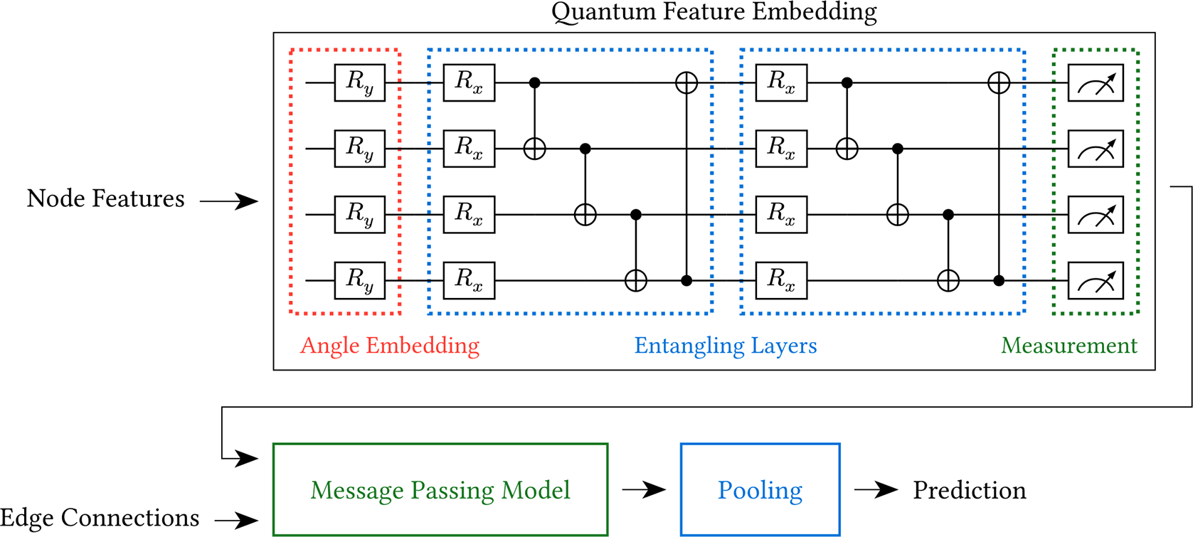
Xu et al. argue that using a VQC to create embeddings provides several benefits. First, because of the unitary nature of the circuit, the norms of the embeddings are preserved. This preservation helps increase the stability of the model during training. The unitary nature of the VQC also implies that it acts as a bijective function, which means that distinct inputs will not be mapped to the same output. This implies that information will not be lost during the embedding process. Finally, the exponential nature of the circuit’s vector space allows the VQC to approximate complex functions with exponentially fewer trainable parameters compared to classical models.

To test QFE empirically, Xu et al. evaluated its performance on the classification problems defined by two benchmark datasets: PROTEINS^5,6 and ENZYMES.^5,7 That performance was then compared with the performance of two classical embedders using Multi-Layer Perceptrons (MLPs). One had $D$ hidden nodes (to approximate the number of parameters in QFE), where $D$ is the number of input features; the other had $2^D$ hidden nodes (to approximate the expressive power of QFE’s vector space). Notably, Xu et al. did not compare QFE with a model with no embedding layer.

Their results, as depicted in Figure 2, led them to conclude that QFE provides an increased accuracy compared to classical models with similar numbers of parameters and can keep up with classical models that have exponentially more parameters.

Figure 2. The results reported by Xu et al. as depicted in their article.³

Note: The State-Of-The-Art (SOTA) performance on PROTEINS is $85.7\%,$⁸ which is much higher than what QFE achieved. However, because QGL and QML in general are young fields, we do not necessarily expect QML models to achieve SOTA performance. Instead, we simply want to determine if the methodology has a positive impact and if it might be useful in the future.

1.2 Our contributions

We critically examine QFE using an improved experimental design with state-of-the-art hyperparameter tuning. This approach yields classical models that perform comparably to QFE and significantly outperform the small classical models used in Xu et al.’s comparison. In addition, we demonstrate that it is possible to obtain similar accuracies with classical models that have fewer trainable parameters.

While this paper may not explore new and exciting QML methodologies, it does provide a rigorous evaluation of an existing technique, which is scientifically valuable. Without negative and critical results like this one, it would be impossible to allocate precious research resources efficiently.

2.1 The embedder

The structure of the individual models we tested remains largely unchanged from the methodology created by Xu et al. During inference, node features are taken from the input graph (or batch of graphs) and passed to the embedder component (if it exists). There are five options for the embedder component:

The QFE embedder, a VQC, starts with an angle embedding component using $R_y$ gates (defined below). This component is used to convert the classical node features into a state the quantum computer can process.

In the entangling component, parameterized $R_x$ gates and controlled not gates (defined below) are combined to create entangling layers which allow the circuit to represent complex functions. The parameters (i.e. the many instances of $\theta$) in these layers are used to update the circuit based on loss calculated between the circuit’s output and the expected output.

The number of layers used in the entangling component is a hyperparameter of our model. As in Xu et al.’s article,³ we finish with a measuring component that measures all of the wires in the quantum circuit.

2.2 The message-passing model

Following that, the embeddings and the edge connections from the input graph are given to the message-passing model. This model can use any type of message-passing layer (including any one of the $66$ convolutional layers provided by the PyTorch Geometric python package⁹). We chose to test the three layer types chosen by Xu et al.³:

The number of hidden channels and the number of layers used by the message-passing model are hyperparameters. The number of output channels is equal to the number of classes in the classification problem.

2.3 Pooling

Next, a pooling layer is used to aggregate the data spread across the nodes of the graph being processed. We tested the three simple options below.

Finally, a log Softmax function is applied.

2.4 Training

During initial training runs, we tried both cross-entropy loss, which was used by Xu et al.,³ and Negative Log Likelihood (NLL) loss, which was used in PyTorch Geometric⁹ examples and in HGP-SL,⁸ the classical model which achieved the SOTA accuracy on the PROTEINS dataset. Both losses produced similar results; we chose to use NLL loss for its popularity.

To optimize the parameters of the entire model (including the QFE embedder, when applicable), we used Adam.¹²

To mitigate overfitting, we implemented early stopping with a patience of $30$ epochs and a maximum training duration of $200$ epochs. The metric used for early stopping is the loss taken from the validation dataset. We also employed dropout, the rate of which is a hyperparameter of the model.

2.5 Hyperparameter tuning

For each embedder option, we optimized our hyperparameters by running a multi-objective Optuna¹³ study that used the Non-dominated Sorting Genetic Algorithm II (NSGA-II) algorithm.¹⁴ Each study included approximately $200$ experiments. Their objectives were to …

The hyperparameters we optimized are listed below.

We also optimized the batch size during our initial experiments. However, since this hyperparameter was shown to have low importance (using the fANOVA evaluation method¹⁵) and since the varying memory usage it caused made it difficult to run experiments in parallel, we ultimately chose to hold it constant at $1024$.

To increase the stability of each experiment within the Optuna¹³ study and obtain an estimate of variability, we performed stratified$$five-fold cross-validation on the provided training dataset and then bootstrapped the accuracies to obtain a $95\%$ confidence interval.

2.6 Cross-validation and testing

Stratified five-fold cross-validation was conducted on the entire dataset to control for the bias caused by our train/test data split and to provide multiple test accuracies which could be used to estimate the variability of the test statistic.

For each of the train/test data splits provided by cross-validation and for each embedder option, we ran hyperparameter tuning and then selected three of the best models produced, each maximizing one of the utility functions below.

To decrease the storage and maintenance burden during hyperparameter tuning and because each model only took a few minutes to train [2], we chose not to save model weights. Instead, we retrained each of the selected models after tuning, this time using a stratified shuffle split to divide the training dataset into a training dataset and a validation dataset (for use during early stopping). To decrease the non-deterministic effects of our training script on the results, we also implemented a minimum training duration of 60 epochs. If early stopping was triggered before then (which likely indicates that training had failed to produce a well-performing model), then the model would be retrained. This could happen up to five times before the training script progresses to the next model.

Finally, we evaluated the selected models from each fold on their corresponding test dataset and then used bootstrapping to calculate a $95\%$ confidence interval for the mean test accuracy.

4.1 PROTEINS

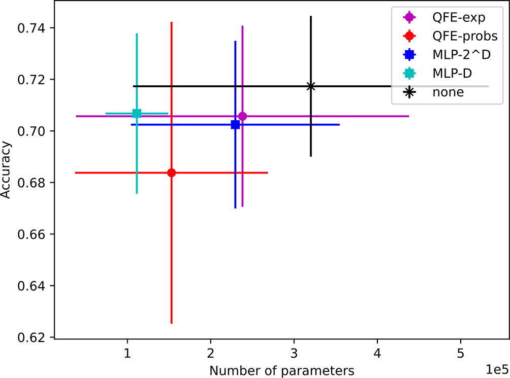
Using $U_{\text{Best Accuracy}}$, we found models with average test accuracies on the PROTEINS dataset ranging from $0.68$ to $0.72$. In particular, we achieved an average accuracy of $0.68$ using the QFE-probs embedder and an average accuracy of $0.71$ using the QFE-exp embedder, both of which are comparable to the results achieved by Xu et al.³ However, we also achieved an average accuracy of $0.71$ using the MLP-$D$ embedder and an average accuracy of $0.72$ using no embedder, which are comparable to the QFE accuracies and significantly higher than the MLP-$D$ accuracies produced by Xu et al.³

The average sizes of our models range from 111K to 320K trainable parameters. Notably, the average number of trainable parameters used by our MLP-$D$-based models is lower than the average for our QFE-based-models (but not significantly lower) even though it exceeds their average accuracies. The results for all five embedder types are depicted with error bars ($\alpha =0.05$) in Figure 5.

Figure 5. Average accuracies and sizes of the models found with $U_{\mathit{\text{Best Accuracy}}}$ on PROTEINS, plotted together with error bars ($\alpha =0.05$).

Unfortunately, Xu et al. did not report their models’ total sizes, so we cannot make direct size comparisons between our models and theirs. They did report the number of floating-point operations (FLOPS) required for MLP-$2^D$ embedder to process a graph with $40$ nodes and the quantum gate operations required for their QFE embedder to process a graph of the same size.^3,18 However, these metrics are not relevant to our analysis since the sizes of the embedders are overshadowed by the variance in the sizes of the message-passing layers.

The models found using $U_{\text{Best}\mathrm{All}}$ performed almost as well as those found with $U_{\text{Best Accuracy}}$, but with an order of magnitude fewer parameters. They achieve accuracies ranging from $0.68$ to $0.71$ with average parameter counts ranging from 13K to 43K. Their results are depicted in Figure 6.

Figure 6. Average accuracies and sizes of the models found with $U_{\mathit{\text{Best}}\mathit{\text{All}}}$ on PROTEINS, plotted together with error bars ($\alpha =0.05$).

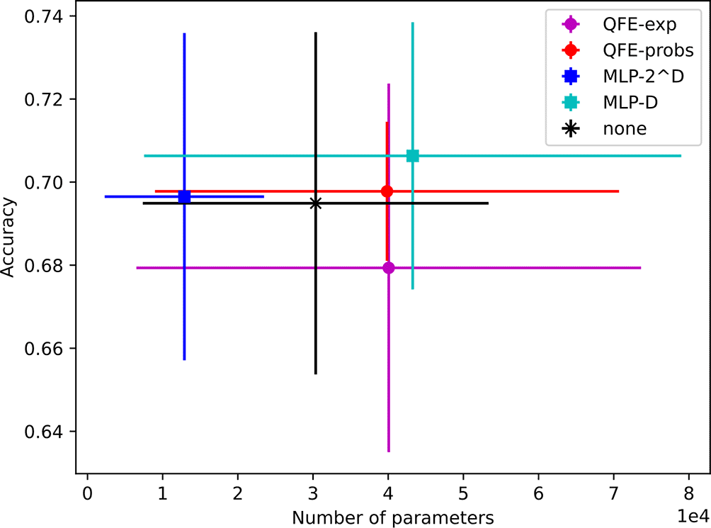
Finally, we found models using $U_{\text{Low}\text{Parameters}}$ that maintain that performance with even fewer parameters. Their average accuracies range from $0.69$ to $0.72$ and their average sizes range from 3K to 11K trainable parameters. Notably, this includes the models using MLP-$2^D$, which maintain an average accuracy of $0.69$ using an average of 3K trainable parameters. The results for all five embedder types are shown in Figure 7.

Figure 7. Average accuracies and sizes of the models found with $U_{\mathit{Low}\mathit{\text{Parameters}}}$ on PROTEINS, plotted together with error bars ($\alpha =0.05$).

4.2 ENZYMES

Our results from ENZYMES represent an even more drastic departure from the results reported by Xu et al. In fact, every single average taken from the models using MLP-$D$ or no embedder is significantly greater than the highest MLP-$D$ accuracy that Xu et al. achieved [3].

The models found using $U_{\text{Best Accuracy}}$ achieve average accuracies ranging from $0.32$ to $0.46$ with average parameter counts ranging from 124K to 299K. Notably, the models with no embedder achieved the highest average accuracy ($0.46$) with an average of 269K trainable parameters. This average is significantly greater than all of the accuracies reported by Xu et al. The results for all five embedders are depicted in Figure 8.

Figure 8. Average accuracies and sizes of the models found with $U_{\mathit{\text{Best Accuracy}}}$ on ENZYMES, plotted together with error bars ($\alpha =0.05$).

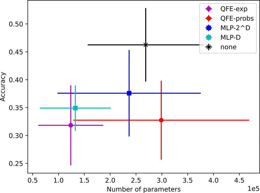
Again, most of the models found using $U_{\text{Best}\mathrm{All}}$ achieve similar average accuracies (although the highest average is no longer $0.46$) using an order of magnitude fewer parameters. Their average accuracies range from $0.26$ to $0.35$ and their average parameter counts range from 18K to 46K. These results are shown in Figure 9.

Figure 9. Average accuracies and sizes of the models found with $U_{\mathit{\text{Best}}\mathit{All}}$ on ENZYMES, plotted together with error bars ($\alpha =0.05$).

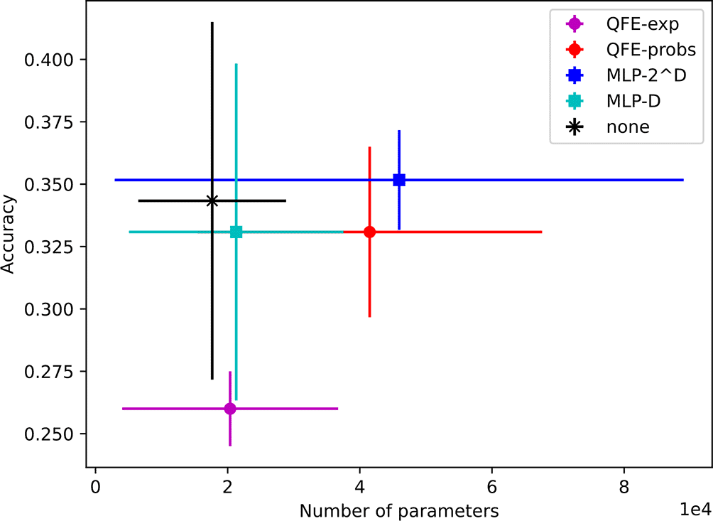
Finally, the models found by $U_{\mathrm{Low}\text{Parameters}}$ achieve similar results with marginally fewer parameters for some and essentially the same number of parameters for others. They achieve accuracies ranging from $0.27$ to $0.40$ with sizes ranging from 3K to 48K trainable parameters. These results are shown in Figure 10.

Figure 10. Average accuracies and sizes of the models found with $U_{\mathit{Low}\mathit{\text{Parameters}}}$ on ENZYMES, plotted together with error bars ($\alpha =0.05$).

5.1 Limitations and future research

There are several limitations (and corresponding future research directions) to this study.