Advanced Numerical Methods for the Fisher-Kolmogorov Reaction-Diffusion Equation: A Quintic Hermite Splines Approach with Richardson Extrapolation

Kedir Aliyi Koroche

doi:10.12688/f1000research.163959.1

Home Browse Advanced Numerical Methods for the Fisher-Kolmogorov Reaction-Diffusion...

ALL Metrics

-

Views

-

Downloads

Get PDF

Get XML

Export

▬

✚

Research Article

Advanced Numerical Methods for the Fisher-Kolmogorov Reaction-Diffusion Equation: A Quintic Hermite Splines Approach with Richardson Extrapolation

[version 1; peer review: awaiting peer review]

Kedir Aliyi Koroche

PUBLISHED 24 Oct 2025

Author details Author details

Mathematics, Ambo University College of Natural and Computational Sciences, Ambo, Oromia, 19, Ethiopia

Kedir Aliyi Koroche
Roles: Conceptualization, Data Curation, Formal Analysis, Funding Acquisition, Investigation, Methodology, Project Administration, Resources, Software, Supervision, Validation, Visualization, Writing – Original Draft Preparation, Writing – Review & Editing

OPEN PEER REVIEW

REVIEWER STATUS AWAITING PEER REVIEW

Abstract

This study introduces a robust numerical method for addressing the fourth-order Fisher-Kolmogorov reaction-diffusion equation, employing a combination of quintic Hermite splines and Richardson extrapolation. The proposed technique effectively transformed the original equation into a system of linear and nonlinear equations, achieving sixth-order convergence in space and fourth-order convergence in time. A thorough stability analysis confirmed the unconditional stability of the method, ensuring that the numerical solutions remained accurate throughout various perturbation scenarios. Extensive numerical experiments validated the performance of the method, revealing significant improvements in accuracy compared to existing approaches. The findings underscore the applicability of the method in mathematical biology and related fields, where the precise modelling of dynamic processes is crucial. Overall, this study contributes to the advancement of numerical techniques for complex differential equations, demonstrating enhanced reliability and precision in computational simulations.

Keywords

Fisher-Kolmogorov Reaction-Diffusion Equation, Quintic Hermite Splines, Richardson Extrapolation, Stability and Convergence of the Method.

Corresponding author: Kedir Aliyi Koroche

Competing interests: No competing interests were disclosed.

Grant information: The author(s) declared that no grants were involved in supporting this work.

Copyright: © 2025 Koroche KA. This is an open access article distributed under the terms of the Creative Commons Attribution License, which permits unrestricted use, distribution, and reproduction in any medium, provided the original work is properly cited. The author(s) is/are employees of the US Government and therefore domestic copyright protection in USA does not apply to this work. The work may be protected under the copyright laws of other jurisdictions when used in those jurisdictions.

How to cite: Koroche KA. Advanced Numerical Methods for the Fisher-Kolmogorov Reaction-Diffusion Equation: A Quintic Hermite Splines Approach with Richardson Extrapolation [version 1; peer review: awaiting peer review]. F1000Research 2025, 14:1160 (https://doi.org/10.12688/f1000research.163959.1) First published: 24 Oct 2025, 14:1160 (https://doi.org/10.12688/f1000research.163959.1) Latest published: 24 Oct 2025, 14:1160 (https://doi.org/10.12688/f1000research.163959.1)

1. Introduction

Various types of non-linear partial differential equations (PDEs) are employed to analyze phenomena in real-life applications, with non-linear advection-diffusion²⁰ and reaction-diffusion equations receiving significant attention (see^20,21,47). These equations have been studied using a variety of numerical methods; however, these techniques often encounter challenges. For instance, Rajan and Reddy¹ proposed a generalized regularization approach to address singularly perturbed parabolic PDEs, which exhibit complex behavior owing to their small perturbation factors. They discussed the characteristics of singular perturbations in parabolic PDEs and the associated numerical challenges, such as boundary layers and steep gradients. Furthermore, the behavior of small solutions in a reaction-diffusion model problem was studied near a co-dimension 2 point in.² The focus on co-dimension 2 points may oversimplify the complex dynamics present in reaction-diffusion models. This could limit the understanding of small solutions and their behaviors in more general contexts. Building on these insights, we introduced a novel regularization strategy aimed at enhancing the solution stability and accuracy by modifying the original PDE to mitigate the effects of singular perturbations.

In addition, numerous researchers have explored various non-linear PDEs using distinct numerical techniques. For example,³ enhanced the numerical analysis of non-linear PDEs, particularly in the context of porous media. Dahab et al.⁴ investigated the behavior of the Casson nanofluid flow over a nonlinearly heated porous medium influenced by magnetic fields (MHD), shedding light on the effects of an extended surface with suction/injection. The numerical solutions for higher-order PDEs in two-dimensional coupled systems were examined using finite difference and finite element methods.⁵ Furthermore, Mebarek⁶ explored the convective heat-transfer properties of titanium nanofluids using various base fluids in a cylindrical annulus with discrete heat sources. Clark and Meyer⁷ focused on two-signed solutions for a specific class of second-order semi-linear parabolic PDEs with non-Lipschitz nonlinearities. Despite these advancements, numerical approaches for solving non-linear PDEs can yield unreliable results owing to their heavy reliance on the initial conditions. Additionally, the complexities of the boundary conditions and high computational demands may restrict their practical applications, highlighting the need for innovative solutions, such as the one we propose.

Building on the highlighted challenges, the application of numerical methods extends to fuzzy nonlinear equations. For instance, Abbasbandy and Asady⁸ presented a variation of Newton’s method tailored for these equations, which is relevant for uncertain systems and decision-making processes. Furthermore, Arora et al.⁹ introduced a stable variable mesh approach for one-dimensional nonlinear parabolic PDEs, and Dehghan et al.¹⁰ developed a numerical simulation technique that integrates the finite element method with proper orthogonal decomposition (POD) to model and mitigate groundwater contamination. Their work emphasized the complexities involved in accurately simulating contamination processes, underscoring how various factors, such as source strength and hydrodynamic conditions, can influence transport dynamics.

In addition to these innovative methodologies, the significance of reaction-diffusion equations is underscored in the work of,¹¹ which provides an overview of the extended Fisher-Kolmogorov equation, particularly relevant in mathematical biology for modeling population dynamics and spreading processes. Further contributions include Samir et al.,¹² who derived exact wave solutions for a fourth-order nonlinear PDE describing the dynamics of optical fiber pulses, thereby revealing implications for optical communication technologies. Knibb and Scraton¹³ presented a collocation method designed for nonlinear parabolic PDEs, which demonstrated advantages over traditional techniques in terms of flexibility and accuracy. Moreover, Abbasbandy¹⁴ demonstrated the effectiveness of the variational iteration method for solving nonlinear Klein-Gordon equations, highlighting its broader potential despite the challenges in convergence and stability when applied to more complex equations.

Continuing this discourse, Gavete et al.¹⁵ discussed an efficient numerical method for second-order nonlinear elliptic PDEs, while Mansour¹⁶ investigated traveling wave solutions for nonlinear reaction-diffusion equations, which are crucial for understanding spatial phenomena across scientific disciplines. Their numerical simulations elucidated how varying parameters influence the behavior of traveling waves, providing insights applicable to population dynamics, chemical reactions, and ecological models. Zhou et al.¹⁷ further explored exact solitary wave solutions for the generalized Fisher equation, which is essential for modeling population dynamics and chemical reactions.

Beitia et al.¹⁸ developed and analyzed effective particle methods for solving Fisher-Kolmogorov equations, which are vital for modeling biological invasion and brain tumor dynamics. Their particle-based numerical method enables the simulation of complex dynamics, emphasizing computational efficiency and flexibility, and yielding insights into tumor growth mechanisms with potential implications for treatment strategies.

However, despite the promising advancements in these studies, we recognize challenges in accurately obtaining solutions for various types of nonlinear reaction-diffusion parabolic equations. Each equation exhibits distinct characteristics that reveal different aspects of biological and physical phenomena. However issues such as the boundary layers, associated perturbation parameters, and nonlinearities complicate the solution process. This underscores the necessity for more effective methods to enhance the solution reliability. In light of these considerations, this study focuses on examining the solutions of a fourth-order nonlinear reaction-diffusion parabolic PDE, known as the Fisher-Kolmogorov equation, with the objective of developing strategies to improve stability and accuracy in the presence of singular perturbations. The fourth-order Fisher-Kolmogorov equation discussed in this paper is presented in the following form:

(1)

u_{t} + β u_{xxxx} - u_{xx} + h (u) = 0, (x, t) \in (a, b) \times (0, T)

where

β > 0

and nonlinear source function

h (u) = u - u^{3}

subjected to the initial and boundary conditions, respectively, is defined as

(2)

\begin{matrix} u (x, 0) = u 0 (x), x \in (a, b); \\ u (a, t) = g_{1} (t), u (b, t) = g_{2} (t); \\ u_{xx} (a, t) = g_{3} (t), u_{xx} (b, t) = g_{4} (t) . \end{matrix}

According to,¹⁹ when $0 < β \leq 1$ , Eq. (1) is called the extended Fisher-Kolmogorov equation: When $β = 0$ , Eq. (1) is termed the standard Fisher-Kolmogorov equation and was developed by Fisher and Kolmogorov to model complex biological processes (see^20,21). According to the investigation in,²² the requirement $β > 0$ was chosen for the stability of this equation at short wavelengths. These findings indicate that the various physical phenomena described by this equation are governed by the perturbation parameter.

Building on this foundational understanding, various physical phenomena, including pattern formation owing to propagating fronts,²³ spatial-temporal chaos in bistable systems,²⁴ chemical waves,²⁵ phase transitions,²⁶ front propagation near Lipschitz points,²⁷ instabilities in liquid crystals,²⁸ and propagating waves in reaction-diffusion systems,²⁹ are described by the EFK equation. According to,³⁰ this equation approaches critical amplitudes near certain degenerate points. Additionally, the transition from periodic patterns predicted by the Ginzburg–Landau equation to multi-bump solutions anticipated by the EFK equation was discussed in.³¹ Furthermore, different investigators have explored various behaviors associated with the EFK equation, such as periodicity,³² chaotic behavior,³³ stationary states,³⁴ solution uniqueness,³⁵ kink existence,³⁶ and traveling wave solutions.

To deepen our understanding of these phenomena, the solution of the EFK equation has been analyzed using variational methods to investigate saddle-focus equilibrium connections (see^37,46). These techniques include a variety of approaches, including the topological shooting method for kink existence and property analysis,³⁸ interpolating element-free Galerkin method,³⁹ orthogonal cubic spline collocation method,⁴⁰ quintic B-spline collocation method,⁴¹ mixed finite element method,¹¹ quintic trigonometric differential quadrature method,⁴² finite element method,⁴³ Galerkin approximation technique,⁴⁴ and compact difference method.⁴⁵ In addition quasi-exact solutions have been explored along with local radial basis functions and finite difference methods (see^46,47), respectively.

Although the analysis of the EFK equation offers valuable insights, it is crucial to acknowledge the limitations of the employed methods. Techniques, such as variational methods and various collocation approaches, often struggle with complex phenomena, including chaotic behavior and traveling wave solutions. For example, mixed finite-element methods frequently encounter issues related to stability and accuracy, particularly near critical points or degenerate regions. Although variational methods provide insights into saddle-focus equilibria, they typically require significant computational resources and may not fully capture the complexities of multibump solutions. This reliance on specific numerical techniques can hinder the generalization of results across different scenarios, complicating the exploration of solution uniqueness and periodicity.

To address these challenges, this study introduces a novel approach that integrates quintic Hermite spline techniques with Richardson extrapolation, aiming to enhance the analysis solutions of the EFK equation. This combined framework seeks to deliver robust solutions that effectively address the complexities of various physical phenomena described by the EFK equation. Quintic Hermite spline methods have shown high-order convergence in solving nonlinear partial differential equations, as evidenced in previous studies (see^48,49). For instance, Arora and Kaur⁵⁰ presented an efficient scheme utilizing quintic Hermite interpolating polynomials for the Burgers equation, which significantly improved both computational accuracy and efficiency. Their subsequent work by Arora et al.⁴⁸ further validated the robustness of quintic Hermite splines, demonstrating their applicability in a variety of fluid dynamics problems. Additionally, Jain et al.⁴⁹ effectively employed collocation methods with quintic Hermite splines to address the Benjamin–Bona–Mahony–Burgers equation, demonstrating the versatility of these techniques in tackling nonlinear phenomena. Furthermore, Alba-Fernández et al.⁵¹ introduced a bootstrap algorithm using trigonometric Hermite spline interpolation, highlighting the utility of the Hermite spline methods in statistical analysis. Collectively, these contributions emphasize the effectiveness and versatility of Hermite spline techniques across both mathematical and applied domains.

Moreover, this work effectively utilizes Richardson extrapolation to enhance the accuracy of numerical solutions. This technique accelerates the accuracy of solutions for various differential equations, as documented in several studies. For instance, Merga and Chemeda⁵² presented a modified Crank-Nicolson scheme that incorporates Richardson extrapolation for the one-dimensional heat equation, significantly improving the solution accuracy and stability. Similarly, Siraj et al.⁵³ applied a fourth-order stable central difference method with Richardson extrapolation to address second-order self-adjoint singularly perturbed boundary-value problems, demonstrating enhanced accuracy in challenging scenarios. Additionally, Chemeda et al.⁵⁴ employed a compact finite-difference scheme with Richardson extrapolation for Fisher’s equation, demonstrating the effectiveness of the method in capturing critical dynamics. Together, these studies highlight the Richardson extrapolation as a powerful technique for enhancing the accuracy and reliability of numerical solutions in various mathematical and engineering contexts.

Based on these findings, the proposed method combines quintic Hermite spline techniques with Richardson extrapolation to offer superior accuracy and stability compared with previously discussed techniques. This approach leverages the smoothness and simplicity of quintic splines, achieving super-convergence and significantly enhancing solution precision. Furthermore, it improves the efficiency of the collocation technique by interpolating the function and its derivatives up to the second order at the nodal sites. Unlike traditional methods, which often struggle with stability and accuracy, this combined approach effectively reduces discretization errors through Richardson extrapolation, making it especially powerful for high-order nonlinear equations. This represents a significant advancement in the numerical analysis of these challenging problems.

This paper also discusses how this method enhances accuracy through a uniform mesh in the temporal direction and a non-uniform mesh in the spatial direction. In addition, it analyzes the traveling wave behavior of the solution using various parameter values and nonlinear source functions. To address these perspectives, the paper is structured as follows: Section 1 introduces the topic; Section 2 formulates the current method; Section 3 discusses the stability and convergence analysis; Section 4 outlines the criteria for measuring the accuracy and rate of convergence of the present method; Section 5 presents numerical experiments; Section 6 discusses and analyzes the findings; and Section 7 concludes the study.

2. Formulating of current numerical techniques

2.1 Quintic Hermit Splines

To address fourth-order non-linear equations, which involve a differential equation alongside four constraints, numerical techniques leverage these constraints to discretize the equation effectively. Specifically, the Quintic Hermite techniques we re employed. Quintic Hermite splines inherently include the discretized form of the differential equation at collocation points along with two boundary constraints for the interpolating polynomial. To obtain such a scheme, the fourth-order differential equation was split into a second-order form by introducing a twice continuously differentiable function, thereby reducing the constraints to two for each interpolating polynomial. To execute this, the following theorem is considered a necessary part of implementing the proposed technique:

Theorem 1:

The Hermite interpolation problem of order $n \in N$ is applicable to two-point boundary value problems.¹⁹

Consider the non-linear EFK type Equation (1). To implement the proposed technique, we introduce a twice continuously differentiable function $v (ζ, t)$ such that:-

v (ζ, t) = - u_{ζζ} (ζ, t) .

As investigated in,⁵⁵ the induced coupled system of differential equations of our governing problem is given as

(3)

v + u_{ζζ} = 0,

(4)

u_{t} - β v_{ζζ} + v + f (u) = 0,

where

f (u) = u - u^{m}

for

m \in ℝ,

subject to the following initial and boundary conditions:

(5)

u (ζ, 0) = u_{0} (ζ),

(6)

u (a, t) = g_{1} (t), u (b, t) = g_{2} (t) .

(7)

v (a, t) = 0, v (b, t) = 0 .

These equations are the transformed forms of EFK into a system comprising one linear equation and one semi-linear equation that involves two functions, u and v.

2.2 The hybrid Quintic Hermite Spline collocation method

The hybrid technique employs semi-discretization methods to discretize both the time and spatial directions. This two-step approach was utilized for a second-order coupled system of singularly perturbed partial differential equations (PDEs):

a. Time discretization

For temporal discretization, we utilized the Crank-Nicolson scheme, a specific instance of the weighted finite difference method, as investigated in.⁵⁶ This scheme takes advantage of the nearest neighboring points to maintain continuity in behavior, avoiding any time discontinuities (see⁵⁷). To apply this technique to the reduced coupled system of the EFK equation, we define the following terms.

Let us consider that both $v^{n + 1}$ and $u^{n + 1}$ are represent the approximating polynomial function at the current time, $t_{n + 1}$ . Also, let $∆ t = \frac{T}{N}, N > 0,$ for $t_{n} = n ∆ t$ for $n = 0, 1, 2, \dots, N$ , be the cell of the time step, and N be the maximum of the sub-interval in the temporal direction. Since, for any function F, we have

(8)

F^{n + \frac{1}{2}} = \frac{F^{n + 1} + F^{n}}{2}

Hence, using the above condition, the semi-discretized forms of our coupled systems are given as

(9)

\begin{matrix} v^{n + \frac{1}{2}} = - u_{ζζ}^{n + \frac{1}{2}} \\ \frac{u^{n + 1} - u^{n}}{∆ t} = β v_{ζζ}^{n + \frac{1}{2}} - v^{n + \frac{1}{2}} - {(u^{n} - u)}^{n + \frac{1}{2}} \end{matrix}

with the corresponding boundary conditions given in Eqs. (6) and (7), respectively.

b. Spatial discretization

Let $a = ζ_{0} < ζ_{1} < ζ_{2} < \dots < ζ_{M} = b,$ where $M$ is the maximum number of subintervals of $I$ in the spatial direction. This indicates that we have a non-uniform grid spacing $ζ_{i} \in I = [a, b]$ for which $h_{i} = ζ_{i + 1} - ζ_{i}$ . Hence, our subintervals are given by $I_{i} = [ζ_{i}, ζ_{i + 1}]$ . For each sub-interval, $I_{i}$ , six collocation points were selected, including two boundary points. These collocation points are the roots of a shifted Legendre polynomial of order six, which is not equidistant from the mean. Details of these collocation points can be found in.⁵⁸ In the spatial direction, we utilized the quintic Hermite interpolating polynomials $p_{i} (ζ)$ , $\bar{p_{i}} (ζ)$ and $\overset{̿}{p_{i}} (ζ)$ that introduced in¹⁹ to approximate the trial function within each partition $I_{i}$ of the solution domain. The approximate function is defined as follows:

(10a)

u (ζ) = u (ζ_{i}) \sum_{i = 1}^{2} P_{i} (ζ) + u^{'} (ζ_{i}) \sum_{i = 1}^{2} \bar{p_{i}} (ζ) + u^{''} (ζ_{i}) \sum_{i = 1}^{2} \overset{̿}{p_{i}} (ζ)

where

p_{i} (ζ)

is the interpolated function

u (ζ)

at each nodal point of sub-interval

I_{i}

and

\bar{p_{i}} (ζ)

and

\overset{̿}{p_{i}} (ζ)

are the interpolated slope and curvature at the nodal points, respectively. As in,¹⁹ they are, respectively, given by

(10b)

\begin{matrix} p_{i} (ζ) = {\begin{matrix} 6 \frac{{(ζ_{i + 1} - ζ)}^{5}}{{(ζ_{i + 1} - ζ_{i})}^{5}} - 15 \frac{{(ζ_{i + 1} - ζ)}^{4}}{{(ζ_{i + 1} - ζ_{i})}^{4}} + 10 \frac{{(ζ_{i + 1} - ζ)}^{3}}{{(ζ_{i + 1} - ζ_{i})}^{3}}, ζ_{i} \leq ζ \leq ζ_{i + 1} \\ 6 \frac{{(ζ - ζ_{i - 1})}^{5}}{{(ζ_{i} - ζ_{i - 1})}^{5}} - 15 \frac{{(ζ - ζ_{i - 1})}^{4}}{{(ζ_{i} - ζ_{i - 1})}^{4}} + 10 \frac{{(ζ - ζ_{i - 1})}^{3}}{{(ζ_{i} - ζ_{i - 1})}^{3}}, ζ_{i - 1} \leq ζ \leq ζ_{i} \\ 0, otherwise \end{matrix}; \\ \bar{p_{i}} (ζ) = {\begin{matrix} 3 \frac{{(ζ_{i + 1} - ζ)}^{5}}{{(ζ_{i + 1} - ζ_{i})}^{4}} - 7 \frac{{(ζ_{i + 1} - ζ)}^{4}}{{(ζ_{i + 1} - ζ_{i})}^{3}} + 4 \frac{{(ζ_{i + 1} - ζ)}^{3}}{{(ζ_{i + 1} - ζ_{i})}^{2}}, ζ_{i} \leq ζ \leq ζ_{i + 1} \\ - 3 \frac{{(ζ - ζ_{i - 1})}^{5}}{{(ζ_{i} - ζ_{i - 1})}^{4}} + 7 \frac{{(ζ - ζ_{i - 1})}^{4}}{{(ζ_{i} - ζ_{i - 1})}^{3}} - 4 \frac{{(ζ - ζ_{i - 1})}^{3}}{{(ζ_{i} - ζ_{i - 1})}^{2}}, ζ_{i - 1} \leq ζ \leq ζ_{i} \\ 0, otherwise \end{matrix}; \\ \overset{̿}{p_{i}} (ζ) = {\begin{matrix} 2 \frac{{(ζ_{i + 1} - ζ)}^{5}}{{(ζ_{i + 1} - ζ_{i})}^{3}} - \frac{{(ζ_{i + 1} - ζ)}^{4}}{{(ζ_{i + 1} - ζ_{i})}^{2}} + 2 \frac{{(ζ_{i + 1} - ζ)}^{3}}{(ζ_{i + 1} - ζ_{i})}, ζ_{i} \leq ζ \leq ζ_{i + 1} \\ 2 \frac{{(ζ - ζ_{i - 1})}^{5}}{{(ζ_{i} - ζ_{i - 1})}^{3}} + \frac{{(ζ - ζ_{i - 1})}^{4}}{{(ζ_{i} - ζ_{i - 1})}^{3}} + 2 \frac{{(ζ - ζ_{i - 1})}^{3}}{{(ζ_{i} - ζ_{i - 1})}^{2}}, ζ_{i - 1} \leq ζ \leq ζ_{i} \\ 0, otherwise \end{matrix} . \end{matrix}

To apply orthogonal collocation within each subinterval $I_{i}$ , a new variable $ω$ is introduced, such that $ω = \frac{ζ - ζ_{i}}{h_{i}}$ where $ω$ varies from $0$ to $1$ as $ζ$ varies from $ζ_{i}$ to $ζ_{i + 1}$ . This transformation reduces the polynomial structure in Eq. (10) into the tabular form shown in Table 1. The Quintic Hermit polynomials are presented in the interval $[ζ_{i}, ζ_{i + 1}]$ in Table 1, and the values of the Hermit splines and their derivatives are presented in Table 2 at $ω = {0, 1}$ . Hence, using this idea, the approximating function at each time $t_{n + 1}$ in each subinterval is taken as

(11)

\begin{matrix} u^{n + 1} (ω) = \sum_{i = 1}^{6} c_{i}^{n + 1} H_{i} (ω) \\ v^{n + 1} (ω) = \sum_{i = 1}^{6} d_{i}^{n + 1} H_{i} (ω) \end{matrix}

where

c_{i}^{n + 1}

and

d_{i}^{n + 1}

are constants of approximations.

Table 1. Presentation of quintic Hermit splines as defined in.¹⁹

$i$	$H_{i}$	${H_{i}}^{'}$	${H_{i}}^{''}$
1	$1 - 10 ω^{3} + 15 ω^{4} - 6 ω^{5}$	$- 30 ω^{2} + 60 ω^{3} - 30 ω^{4}$	$- 60 ω + 180 ω^{2} - 120 ω^{3}$
2	$h (ω - 6 ω + 8 ω^{4} - 3 ω^{5})$	$h (1 - 18 ω^{2} + 32 ω^{3} - 15 ω^{4})$	$h (- 36 ω + 96 ω^{2} - 60 ω^{3})$
3	$\frac{h^{2}}{2} (ω^{2} - 3 ω^{3} + 3 ω^{4} - ω^{5})$	$\frac{h^{2}}{2} (2 ω - 9 ω^{2} + 12 ω^{3} - 5 ω^{4})$	$\frac{h^{2}}{2} (2 - 18 ω + 36 ω^{2} - 20 ω^{3})$
4	$\frac{h^{2}}{2} (ω^{3} - 2 ω^{4} + ω^{5})$	$\frac{h^{2}}{2} (3 ω^{2} - 8 ω^{3} + 5 ω^{4})$	$\frac{h^{2}}{2} (6 ω - 24 ω^{2} + 20 ω^{3})$
5	$10 ω^{3} - 15 ω^{4} + 6 ω^{5}$	$30 ω^{2} - 60 ω^{3} + 30 ω^{4}$	$60 ω - 180 ω^{2} + 120 ω^{3}$
6	$h (- 4 ω^{3} + 7 ω^{4} - 3 ω^{5})$	$h (- 12 ω^{2} + 28 ω^{3} - 15 ω^{4})$	$h (- 24 ω + 84 ω^{2} - 60 ω^{3})$

Table 2. Value of quintic Hermite splines and corresponding first and second order derivatives at boundary points as evaluated in.¹⁹

$i$	$H_{i}$		$H_{i}^{'}$		$H_{i}^{''}$
$i$	$ω = 0$	$ω = 1$	$ω = 0$	$ω = 1$	$ω = 0$	$ω = 1$
$1$	$1$	$0$	$0$	$0$	$0$	$0$
$2$	$0$	$0$	$h$	$0$	$0$	$0$
$3$	$0$	$0$	$0$	$0$	$h^{2}$	$0$
$4$	$0$	$0$	$0$	$0$	$0$	$h^{2}$
$5$	$0$	$1$	$0$	$0$	$0$	$0$
$6$	$0$	$0$	$0$	$h$	$0$	$0$

The process of selecting collocation points is crucial in the Hermit collocation methods. To obtain these colocation points, we use the zeros of the orthogonal polynomials called Jacobi polynomials. The Legendre and Chebyshev polynomials are special cases of Jacobi polynomials. Hence, in this study, we utilized the zeros of the shifted Legendre polynomials as collocation points.

However, at each of these collocation points, the semi-discretization of the aforementioned equation by substituting Eq. (8) into Eq. (9) in the coupled system, we obtain

(12)

\begin{matrix} \frac{v^{n + 1} + v^{n}}{2} = - [\frac{u_{ζζ}^{n + 1} + u_{ζζ}^{n}}{2}] \\ u^{n + 1} - u^{n} = β ∆ t [\frac{v_{ζζ}^{n + 1} + v_{ζζ}^{n}}{2}] - ∆ t [\frac{v^{n + 1} + v^{n}}{2}] - \frac{∆ t}{2} [f^{n + 1} (u) + f^{n} (u)] . \end{matrix}

As investigated in,⁵⁹ the quasi-linearization of $f (u) = u^{m} - u$ where $m \in ℝ$ has been obtained using the Taylor series approximation, and it is given as

(13)

\begin{matrix} u^{m} (t + ∆ t) = u^{m} (t) + ∆ t {(u^{m})}_{t} + O {(∆ t)}^{2} \\ = u^{m} (t) + ∆ tm u^{m - 1} u_{t} + O {(∆ t)}^{2} \end{matrix}

By using finite difference approximation of $u (t + ∆ t)$ with order two, we have:

u (t + ∆ t) = u (t) + ∆ t u_{t} + O {(∆ t)}^{2}

Then, neglecting ${(∆ t)}^{2}$ , this equation gives us:

(14)

u_{t} = \frac{u (t + ∆ t) - u (t)}{∆ t}

Substituting Eq. (14) into Eq. (13), at $t = t_{n}$ , we obtain

\begin{matrix} u^{m} (t_{n} + ∆ t) = u^{m} (t_{n}) + m u^{m - 1} (u (t_{n} + ∆ t) - u (t_{n})) + O {(∆ t)}^{2} \\ = u^{m} (t_{n}) + m u^{m - 1} u (t_{n} + ∆ t) + m u^{m} (t_{n}) + O {(∆ t)}^{2} . \end{matrix}

By approximating the value of $u (t_{n + 1})$ from the above difference equation, we obtain:

(15)

u (t_{n + 1}) = u^{m} (t_{n}) + m u^{m - 1} u (t_{n} + ∆ t) + m u^{m} (t_{n}) + O {(∆ t)}^{2} .

Using Eq. (15) in Eq. (12) after neglecting the second-order truncation term, we obtain

\frac{v^{n + 1} + u_{ζζ}^{n + 1}}{2} = - \frac{(v^{n} + u_{ζζ}^{n})}{2} u^{n + 1} - u^{n} = β ∆ t (\frac{v_{ζζ}^{n + 1} + v_{ζζ}^{n}}{2}) - ∆ t (\frac{v^{n + 1} + v^{n}}{2}) + ∆ t (\frac{u^{n + 1} + u^{n}}{2}) - \frac{∆ t}{2} ({mu}^{n + 1} {(u^{m - 1})}^{n} - (m - 2) u^{mn}) .

By rearranging the terms, we obtain the coupled system of equations given by:

(16)

\begin{matrix} v^{n + 1} + u_{ζζ}^{n + 1} = - v^{n} - u_{ζζ}^{n} \\ u^{n + 1} + \frac{∆ t}{2} (v^{n + 1} + {mu}^{n + 1} {(u^{m - 1})}^{n} - u^{n + 1} - β v_{ζζ}^{n + 1}) = u^{n} + \frac{∆ t}{2} (β v_{ζζ}^{n} + (m - 2) u^{mn} + u^{n} - v^{n}) \end{matrix}

Since, from Eq. (11), the discretization of both $u^{n + 1}$ and $v^{n + 1}$ in the spatial direction for $0 \leq ω \leq 1$ is given by $u^{n + 1} = \sum_{i = 1}^{6} c_{i}^{n} H_{i} (ω)$ ;

(17)

v^{n + 1} = \sum_{i = 1}^{6} d_{i}^{n} H_{i} (ω) .

Since we know that The approximate solution lies in each subinterval $I_{i}$ , where $H_{i} (ω)$ are quintic Hermite splines defined over the interval [0, 1]. Therefore, using this concept and Eq. (17), the system of collocation equations obtained after discretization is explained as follows:

(18)

\sum_{i = 1}^{6} {c_{4 (r - 1) + i}^{n + 1} K_{ji} + d_{4 (r - 1) + i}^{n + 1} η_{ji}} = \sum_{i = 1}^{6} {c_{4 (r - 1) + i}^{n} ν_{ji} + d_{4 (r - 1) + i}^{n} α_{ji}}

(19)

\sum_{i = 1}^{6} {c_{4 (r - 1) + i}^{n + 1} ρ_{ji} + d_{4 (r - 1) + i}^{n + 1} γ_{ji}} = \sum_{i = 1}^{6} {c_{4 (r - 1) + i}^{n} χ_{ji} + d_{4 (r - 1) + i}^{n} λ_{ji}} + \frac{(m - 2) Δ t}{2} {[\sum_{i = 1}^{6} c_{4 (r - 1) + i}^{n} H_{i} (ω)]}^{m}

where

r = 1 (1) M

,

j = 1 (1) 4

,

c_{i}, & d_{i}

are the unknown coefficients to be determined. The constant parameters are defined as in,¹⁹ and are given by

(20)

\begin{matrix} ρ_{ji} = H_{i} (ω_{j}) - \frac{Δt}{2} H_{i} (ω_{j}) + \frac{mΔt}{2} H_{i} (ω_{j}) {[\sum_{i = 1}^{6} c_{4 (r - 1) + i}^{n} H_{i} (ω_{j})]}^{m}; \\ K_{ji} = \frac{1}{2 h^{2}} H''_{i} (ω_{j}), η_{ji} = \frac{1}{2} H_{i} (ω_{j}), α_{ji} = \frac{- 1}{2} H_{i} (ω_{j}); \\ \begin{matrix} γ_{ji} = \frac{- βΔt}{2 h^{2}} H''_{i} (ω_{j}) + \frac{Δt}{2} H_{i} (ω_{j}); λ_{ji} = \frac{βΔt}{2 h^{2}} H''_{i} (ω_{j}) - \frac{Δt}{2} H_{i} (ω_{j}); \\ χ_{ji} = H_{i} (ω_{j}) + \frac{Δt}{2} H_{i} (ω_{j}), ν_{ji} = \frac{- 1}{2 h^{2}} H''_{i} (ω_{j}) . \end{matrix} \end{matrix}

The total number of variables was 8M + 4, and the collocation equations were 8M. The additional four variables are computed from the boundary conditions of the system of equations. Therefore, by introducing a vector of unknown variables, the compact form of the system of difference equations is

(21)

[A] Y^{n + 1} = [B] Y^{n} + f^{n}

where $A$ and $B$ are $8 M \times 8 M$ diagonally dominated matrices with each block $A_{r}$ and $B_{r}$ for $r = 2, \dots, M - 1$ of order $8 \times 12$ and they are given as:

Y^{n} = {[\begin{matrix} d^{n} (i) \\ c^{n} (i) \end{matrix}]}_{8 M \times 1}, d^{n} = {[\begin{matrix} d_{1}^{n} \\ d_{2}^{n} \\ \begin{matrix} ⋮ \\ d_{4 M}^{n} \end{matrix} \end{matrix}]}_{4 M \times 1}, c^{n} = {[\begin{matrix} c_{1}^{n} \\ c_{2}^{n} \\ \begin{matrix} ⋮ \\ c_{4 M}^{n} \end{matrix} \end{matrix}]}_{4 M \times 1},

A = {[\begin{matrix} \begin{matrix} \begin{matrix} \begin{matrix} A_{1} \end{matrix} \end{matrix} \\ \begin{matrix} \begin{matrix} \begin{matrix} A_{2} \end{matrix} \end{matrix} \end{matrix} \end{matrix} & \begin{matrix}  \end{matrix} \\ ⋱ \\ \begin{matrix} \begin{matrix} \begin{matrix} \begin{matrix} \begin{matrix}  \end{matrix} \end{matrix} & \begin{matrix} \begin{matrix}  \end{matrix} \end{matrix} \end{matrix} & \begin{matrix} \begin{matrix}  \end{matrix} \end{matrix} \end{matrix} & \begin{matrix} A_{r} \\ \begin{matrix}  \end{matrix} \end{matrix} \end{matrix} & \begin{matrix} \begin{matrix} ⋱ \end{matrix} \end{matrix} & \begin{matrix} \begin{matrix} A_{M} \end{matrix} \end{matrix} \end{matrix}]}_{8 M \times 8 M}, B = {[\begin{matrix} \begin{matrix} \begin{matrix} \begin{matrix} \begin{matrix} B_{1} \end{matrix} \end{matrix} \end{matrix} \\ \begin{matrix} \begin{matrix} \begin{matrix} B_{2} \end{matrix} \end{matrix} \end{matrix} \end{matrix} & \begin{matrix}  \end{matrix} \\ ⋱ \\ \begin{matrix} \begin{matrix} \begin{matrix} \begin{matrix} \begin{matrix}  \end{matrix} \end{matrix} & \begin{matrix} \begin{matrix}  \end{matrix} \end{matrix} \end{matrix} & \begin{matrix} \begin{matrix}  \end{matrix} \end{matrix} \end{matrix} & \begin{matrix} B_{r} \\ \begin{matrix}  \end{matrix} \end{matrix} \end{matrix} & \begin{matrix} \begin{matrix} ⋱ \end{matrix} \end{matrix} & \begin{matrix} \begin{matrix} B_{N} \end{matrix} \end{matrix} \end{matrix}]}_{8 M \times 8 M};

and the source term

f^{n}

contains both the nonlinear term

\frac{(m - 2) Δ t}{2} {[\sum_{i = 1}^{6} c_{4 (r - 1) + i}^{n} H_{i} (ω)]}^{m}

and the non-homogeneous boundary data points of the functional values. It is given by:

fn = [\begin{matrix} \begin{matrix} 0 \\ \frac{(m - 2) Δ t}{2} {[\sum_{i = 1}^{6} c_{i}^{n} H_{i} (ω_{j})]}^{m} \end{matrix} \\ \begin{matrix} ⋮ \\ 0 \\ \frac{(m - 2) Δ t}{2} {[\sum_{i = 1}^{6} c_{4 (r - 1) + i}^{n} H_{i} (ω_{j})]}^{m} \end{matrix} \\ \begin{matrix} ⋮ \\ 0 \\ \frac{(m - 2) Δ t}{2} {[\sum_{i = 1}^{6} c_{4 (M - 1) + i}^{n} H_{i} (ω_{j})]}^{m} \end{matrix} \end{matrix}]

Each block matrix, $A_{r}$ and $B_{r}$ also contained a sub-block matrix of order $2 \times 2 .$ The block matrices $A_{r}$ and $B_{r}$ having the following structures:

A_{r} = [{[\begin{matrix} η_{ji} & K_{ji} \\ γ_{ji} & ρ_{ji} \end{matrix}]}_{ij}], B_{r} = [{[\begin{matrix} α_{ji} & ν_{ji} \\ λ_{ji} & χ_{ji} \end{matrix}]}_{ij}]

where

i = 1, 2, 3, 4

and

j = 1, 2, \dots, 6

except for the case of r = 1 and

M

due to known boundary data. This means that for known boundary constraints, all block matrixes

, A_{1}

,

A_{M}, B_{1}

, and

B_{r}

have an order

8 \times 10 .

Hence, from Eq. (21),

Y^{n + 1}

is

8 M \times 1

column vectors given by.

(22)

Y^{n + 1} = [A^{- 1} B] Y^{n} + [A^{- 1} f^{n}]

After determining the unknown parameters $c_{i}, & d_{i}$ from the coupled system of difference equations in Eq. (22), we can determine the discretized functional values $u^{n + 1}$ and $v^{n + 1}$ in the spatial direction by applying Eq. (17).

However, in the numerical scheme above, the presence of a non-linear term may lead to error propagation during the iteration process to solve the problem. Therefore, we mitigated this issue by linearizing our coupled system of difference equations.

2.3 Linearization of discretized scheme

Let u be considered a locally constant value, denoted as μ, for quasi-linearization of the non-linear term. The implemented technique involves operators Ψ and Φ, which operate on u and v, given as $Ψ_{u, v}$ and $Φ_{u, v}$ respectively. This operator approximates two sets of values for each iteration at the selected collocation points for the two approximate solutions, ŭ and $\overset{˘}{v}$ . This means that the iterative scheme at each time step approximates a function comprising two component functional values $U = {u, v}$ . To obtain this approximate function using the scheme, we employed the component Hermite interpolating polynomial, defined as follows: $H = {\overset{˘}{H_{1}}, \overset{˘}{H_{2}}}$ on $C^{6} [a, b]$ . Let u be the bounded functional value. The operators can then be linearized by considering: $μ = max_{m, n} {[u (t_{n})]}^{m - 1}$ .

We assume that $\overset{˘}{U} = {\overset{˘}{u}, \overset{˘}{v}}$ is an approximation of $U = {u, v}$ . As investigated in,¹⁹ we applied the Crank-Nicolson discretization scheme to our operators, which are given as follows:

(23a)

\begin{matrix} Ψ_{u, v} (ω_{i}) = P_{1} (u^{j} (ω_{i}), v^{j} (ω_{i})); \\ Φ_{u, v} (ω_{i}) = P_{2} (u^{j} (ω_{i}), v^{j} (ω_{i})); \end{matrix}

where

Ψ (U (ω_{i})) \approx Ψ_{u, v} (ω_{i}) = v^{j + 1} (ω_{i}) + u_{ζζ}^{j + 1} (ω_{i})

Φ (U (ω_{i}) \approx Φ_{u, v} (ω_{i})) = u^{j + 1} (ω_{i}) - \frac{∆ t}{2} (β v_{ζζ}^{j + 1} (ω_{i}) - v^{j + 1} (ω_{i}) + (1 - mμ) u^{j + 1} (ω_{i}));

P_{1} (u^{j} (ω_{i}), v^{j} (ω_{i})) ≅ - v^{j} (ω_{i}) - u_{ζζ}^{j} (ω_{i});

P_{2} (u^{j} (ω_{i}), v^{j} (ω_{i})) ≅ u^{j} (ω_{i}) + \frac{∆ t}{2} (β v_{ζζ}^{j} (ω_{i}) - v^{j} (ω_{i}) + (1 - mμ) u^{j} (ω_{i}))

j = 0, 1, 2, \dots, N & i = 0, 1, 2, \dots, M .

The matrix notation for the parameters and collocation equations can be expressed as follows:

(23b)

A Y^{j + 1} = [\begin{matrix} Ψ_{u, v} \\ Φ_{u, v} \end{matrix}], B Y^{j} = [\begin{matrix} P_{1}^{j} \\ P_{2}^{j} \end{matrix}], Y^{j} = [\begin{matrix} d_{i}^{j} \\ c_{i}^{j} \end{matrix}]

where

Y^{j}

contains the coefficients of Hermite polynomials. In this approximation technique, both A and B are symmetrical and diagonally dominant. Consequently, every symmetric and diagonally dominant matrix is positive definite. Thus, by employing the Gauss-Seidel iterative method, we can determine the unknown coefficients of Hermite polynomials.

2.4 Order of the proposed method

Because, to discretize Eq. (1), the Crank-Nicolson scheme is applied to discretize the temporal derivative, which has a second-order accurate numerical technique, as indicated in Eq. (13). Subsequently, the quintic hermite spline collocation technique was employed in the spatial direction. The degree of the interpolated quintic hermite splines function on the collocation points is six. Thus, the numerical method resulting from this interpolation has 6th-order-accurate as shown in Eq. (10) in a specific direction. Therefore, by combining these cases, the method proposed in Eq. (16) exhibits a six-order accuracy in the spatial direction and a second-order accuracy in the temporal direction. This implies that the order of accuracy of the proposed method is $O (h^{6} + ∆ t^{2}) .$

2.5 Application of Richardson Extrapolation

One advantage of the RE technique is that it enhances the accuracy of the approximate solutions for given differential equation (see^52,60). It is also used to accelerate the convergence of the underlying method in solving the provided equation (see⁵³).

However, the goal of this extrapolation is to apply the difference scheme to two consecutive grids and then combine the resulting solutions to achieve higher-order approximations (see^54,61). To do this, let us consider a set containing consecutive grid points, which are called $Ω_{h_{i}}^{∆ t}$ coarser and $Ω_{h_{i}}^{∆ t / 2}$ finer points that are defined on the grid points of the temporal direction. Hence, at each and every one of these grid points, we can obtain a numerical solution of Eq. (1) using the following difference equations:

(24a)

u_{h_{i}}^{∆ t} = u^{m} (t_{n}) + m u^{m - 1} u (t_{n} + ∆ t) + m u^{m} (t_{n}) + C ∆ t^{2} + R (h_{i}, ∆ t), (x_{i}, t_{n}) \in Ω_{h_{i}}^{∆ t} .

(24b)

u_{h_{i}}^{∆ t / 2} = u^{m} (t_{n}) + m u^{m - 1} u (t_{n} + ∆ t) + m u^{m} (t_{n}) + \frac{C}{2} ∆ t^{2} + R (h_{i}, ∆ t / 2), (x_{i}, t_{n}) \in Ω_{h_{i}}^{∆ t / 2}

where

R (h_{i}, ∆ t)

and

R (h_{i}, ∆ t / 2)

are the remainders of order

O (h^{6} + ∆ t^{4})

and C is a constant independent of h and

∆ t

. To eliminate

C ∆ t^{2}

, Eq. (24a) by

- 1 / 15

and Eq. (24b) by

16 / 15

and combining the results, we obtain a more accurate approximate solution using the formulas given by

(25a)

u (t_{n}) = \frac{16 u_{h_{i}}^{∆ t / 2} - u_{h_{i}}^{∆ t}}{15} + O (h^{6} + ∆ t^{4}), (x_{i}, t_{n}) \in Ω_{h_{i}}^{∆ t}

This can be extended to both $v$ and $u .$ Based on Eq. (16), we define the values of $V$ and $U$ as:

V_{n} = v^{n} + u_{ζζ}^{n}

U_{n} = u^{n} + \frac{∆ t}{2} (β v_{ζζ}^{n} + (m - 2) u^{mn} + u^{n} - v^{n})

Now using Richardson Extrapolation Formula, we have:

V (t_{n}) = \frac{2^{p} V_{h_{i}}^{n / 2} - V_{h_{i}}^{n}}{2^{p} - 1} + O (h^{6} + ∆ t^{p})

U (t_{n}) = \frac{2^{p} U_{h_{i}}^{n / 2} - U_{h_{i}}^{n}}{2^{p} - 1} + O (h^{6} + ∆ t^{p})

where

p

is the order of convergence,

∆ t / 2 \approx n / 2

, V

(t_{n})

and U

(t_{n})

represent the extrapolated values of

v

and

u

at time

t_{n}

,

V_{h_{i}}^{n / 2}

and

U_{h_{i}}^{n / 2}

are their approximations values using a smaller time step

∆ t / 2

,

V_{h_{i}}^{n}

and

U_{h_{i}}^{n}

are the approximations using the original time step

∆ t

respectively. In our case, the order of convergence for the time variable was

= 4 .

Using this and cutting off the truncation error, the extrapolation for V is given by

(25b)

V (t_{n}) = \frac{16 V_{h_{i}}^{n / 2} - V_{h_{i}}^{n}}{15}

Again, by eliminating the truncation error, the extrapolation of U is given by

(25c)

U (t_{n}) = \frac{16 U_{h_{i}}^{n / 2} - U_{h_{i}}^{n}}{15}

where V

(t_{n})

and U

(t_{n})

represent the improved approximations for velocity and displacement, respectively, based on the values computed at the original and halved time steps.

These schemes demonstrate that the order of accuracy of the proposed scheme increases by two in the temporal direction after applying the Richardson extrapolation process. This means that the accuracy of the present scheme improved to the sixth order in the spatial direction and fourth order in the temporal direction following the Richardson extrapolation. The order of accuracy can be expressed as $O (h^{6} + ∆ t^{4}) .$ This demonstrates that applying Richardson extrapolation doubles the convergence rate of the proposed scheme compared to that of the original scheme.

3. Stability and convergence analysis

For any numerical technique involving iterations for analyzing transient partial differential equations, stability is one of the most important concepts to be considered to ensure control over errors. Otherwise, the accumulation of errors in one stage may overwhelm the solution. Therefore, we must analyze the stability of our numerical method to determine its convergence.

However, the stability of the proposed hybrid numerical algorithm was completely stored in the component matrices of $[A^{- 1} B]$ which improved the initial solution at each iteration. Consequently, the component matrices A and B depend on the perturbation parameters, grid sizes toward both the spatial and time directions, and Hermite splines adopted for approximation. Therefore, to analyze the stability of the current method, we can identify the magnitude of the eigenvalue of matrix $[A^{- 1} B]$ in the side-unit circle.

Based on this idea, let us consider λ as the eigenvalue of the matrix $[A^{- 1} B]$ . So, we observe computationally, the magnitude of these eigenvalues must be bounded by unity. It means we must show the Lax–Richtmyer definition for stability criteria. (i.e $| λ | \leq 1$ ). To show this stability condition we use Lyapunov stability techniques. Another requirement of stability analysis techniques is Von Neumann stability analysis techniques. This technique requires the linearity of the difference equations (see⁶²). So, due to this case, we use Lyapunov stability techniques to analyze the stability of the current numerical scheme. To do this, let us consider the following lemma and theorems given below.

Definition 1:

If the amplification factor associated with the eigenvalues of the coefficient matrices is bounded, this typically indicates that the system of equations is stable.

Lemma 1:

In the proposed difference scheme, given in Eq. (22), all the sequences of $f^{n}$ are bounded.

Proof:

Let us assume that the sequence $Y^{n}$ is bounded. This means that there exists a constant $M_{Y}$ such that

‖ Y^{n} ‖ \leq M_{Y} for all n .

We know that $A^{- 1}$ is a matrix that transforms vector $Y^{n}$ . If A is invertible, then $A^{- 1}$ is bounded. Therefore, there exists a constant $M_{A} > 0$ such that

‖ A^{- 1} ‖ \leq M_{A}

This holds true, because A is a diagonally dominant matrix. Every diagonal dominant matrix is invertible.

Using the triangular inequality, the first term on the right-hand side can be bounded as follows:

∥ A^{- 1} B Y^{n} ∥ \leq ∥ A^{- 1} ∥ ∥ B ∥ ∥ Y^{n} ∥ \leq M_{A} ∥ B ∥ M_{Y} .

Let $M_{1} = M_{A} ∥ B ∥ M_{Y}$ . Thus, $∥ A^{- 1} B Y^{n} ∥ \leq M_{1}$ .

Now consider the second term in the right hand side, we have:

∥ A^{- 1} f^{n} ∥ \leq ∥ A^{- 1} ∥ ∥ f^{n} ∥ \leq M_{A} ∥ f^{n} ∥ .

Combining both terms, we have:

∥ Y^{n + 1} ∥ \leq ∥ A^{- 1} B Y^{n} ∥ + ∥ A^{- 1} f^{n} ∥ \leq M_{1} + M_{A} ∥ f^{n} ∥ .

Hence, if $Y^{n}$ is bounded, to prevent $Y^{n + 1}$ from becoming unbounded, $f^{n}$ must also be bounded. Therefore, for a unique constant $M_{Y}$ , we have

M_{1} + M_{A} ∥ f^{n} ∥ \leq M_{Y}

Therefore, this show that $f^{n}$ is bounded as $n \to \infty .$

Theorem 2:

If each amplification factor of the linear-difference equation in Eq. (22) is bounded, the system of difference equations is stable.

Proof:

To prove this theorem, we utilize Von Neumann’s stability criteria. We assume that the magnitudes of all eigenvalues of $A^{- 1} B$ and the sequence $A^{- 1} G^{j}$ are bounded, where $f^{j} \approx G^{j}$ at $j^{th}$ iterative value. Therefore, for $Ζ^{j} \approx Y^{j}$ , the system can be rewritten as a first-order difference equation of the form

(26)

Ζ^{j + 1} = A^{- 1} B Ζ^{j} + A^{- 1} G^{j} .

where

j = 0, 1, 2, \dots, N .

Assume that the solution to the difference equation in Eq. (26) can be expressed as a Fourier series expansion as follows:

(27)

Ζ^{j} = \sum_{k} Ζ_{k} e^{\frac{i 2 πkj}{N}};

where

i = \sqrt{- 1}, Ζ_{k}

are the Fourier coefficients, and N is maximum number of grid points in temporal direction. Then, substituting Eq. (26) into Eq. (27), we obtain

(28)

\begin{matrix} \sum_{k} Ζ_{k}^{j + 1} e^{\frac{i 2 πkj}{N}} = A^{- 1} B \sum_{k} Ζ_{k}^{j} e^{\frac{i 2 πkj}{N}} + A^{- 1} G^{j}; \\ \sum_{k} Ζ_{k}^{j + 1} e^{\frac{i 2 πkj}{N}} = \sum_{k} A^{- 1} {BΖ}_{k}^{j} e^{\frac{i 2 πkj}{N}} + A^{- 1} G^{j} \end{matrix}

By equating the coefficients of the exponential terms, we defined the amplification factor, denoted as $Λ_{k}$ . This factor represents the ratio of the Fourier coefficients at two consecutive time steps, given by

(29)

Λ_{k} = Ζ_{k}^{j + 1} / Ζ_{k}^{j}

Now, using Eq. (29) in Eq. (28) and simplifying the results, we obtain

(30)

Λ_{k} = A^{- 1} B + A^{- 1} G^{j} / Ζ_{k}^{j}

By applying the triangular inequality on Eq. (30), we obtain:

‖ Λ_{k} ‖ = ‖ A^{- 1} B + \frac{A^{- 1} G^{j}}{Ζ_{k}^{j}} ‖ \leq ‖ A^{- 1} B ‖ + ‖ \frac{A^{- 1} G^{j}}{Ζ_{k}^{j}} ‖

To show that $‖ Λ_{k} ‖$ is bounded, we draw on the principles established in the proof of Lemma 1. Here, is structured argument.

Because $A$ is a diagonally dominant matrix, $A^{- 1} B$ is bounded, which means that by Lemma 1, there exists a constant $M_{A}$ such that

∥ A^{- 1} ∥ \leq M_{A}

Consequently, we can assert that:

(i)

‖ A^{- 1} B ‖ \leq ‖ A^{- 1} ‖ ‖ B ‖ \leq M_{A} ‖ B ‖

Hence, $A^{- 1} B$ is bounded. Again, by Lemma 1, assuming $Ζ_{k}^{j}$ is bounded and nonzero (to prevent division by zero), there exists a constant $M_{Z}$ such that

‖ Ζ_{k}^{j} ‖ \geq M_{Z} > 0

Thus, we can write:

(ii)

‖ \begin{matrix} \frac{A^{- 1} G^{j}}{Ζ_{k}^{j}} \end{matrix} ‖ \leq \frac{‖ A^{- 1} G^{j} ‖}{M_{Z}}

From the properties of $A^{- 1}$ :

‖ A^{- 1} G^{j} ‖ \leq ‖ A^{- 1} ‖ ‖ G^{j} ‖ \leq M_{A} ‖ G^{j} ‖

Therefore, combining this to (ii), we obtain:

(iii)

‖ \begin{matrix} \frac{A^{- 1} G^{j}}{Ζ_{k}^{j}} \end{matrix} ‖ \leq \frac{‖ A^{- 1} G^{j} ‖}{M_{Z}} \leq \frac{‖ A^{- 1} ‖ ‖ G^{j} ‖}{M_{Z}} < \frac{M_{A} ‖ G^{j} ‖}{M_{Z}}

Substituting inequalities (i) and (ii) into the triangular inequalities above, we obtain:

‖ Λ_{k} ‖ = ‖ A^{- 1} B + \frac{A^{- 1} G^{j}}{Ζ_{k}^{j}} ‖ \leq ‖ A^{- 1} B ‖ + ‖ \frac{A^{- 1} G^{j}}{Ζ_{k}^{j}} ‖ < M_{A} ‖ B ‖ + \frac{M_{A} ‖ G^{j} ‖}{M_{Z}}

This shows that $‖ Λ_{k} ‖$ is bounded for all k as long as $‖ B ‖$ and $‖ G^{j} ‖$ are bounded and $Ζ_{k}^{j}$ remains nonzero and bounded. This aligns with the findings of Lemma 1, where boundedness is established under the necessary conditions. Hence, according to Definition 1, the proposed system of difference equations is stable.

Theorem 3:

If the eigenvalues of $A^{- 1} B$ and sequence $A^{- 1} G^{j}$ are bounded, then the difference equation in Eq. (22) is asymptotically stable at all the equilibrium points within the solution domain.

Proof:

To prove this theorem, we use Lyapunov stability analysis techniques. Now, we express the difference equation as a first-order difference equation.

(31)

Ζ^{j + 1} = A^{- 1} B Ζ^{j} + A^{- 1} G^{j}

Let $Ζ^{j + 1} ≅ Ζ^{j} \approx Z_{e}$ be an equilibrium point within the solution domain. From Eq. (31), at equilibrium, we have

(32)

Z_{e} = {[I - A^{- 1} B]}^{- 1} A^{- 1} G^{j}

where

I

denotes an identity matrix. In this equation, it is assumed that (

I - A^{- 1} B

) is invertible and the equilibrium point

Z_{e}

is well defined.

Choose a Lyapunov function $L (Z^{j})$ that satisfies the following conditions:

L (Z^{j}) = {(Z^{j} - Z_{e})}^{T} (Z^{j} - Z_{e}) .

This function satisfies the conditions $L (Z^{j}) \geq 0$ for all $Z^{j}$ , and $L (Z^{j}) = 0$ if and only if $Ζ^{j} \approx Z_{e} .$

The difference between successive values of the Lyapunov function can then be expressed by expanding the results using Eq. (31), we obtain

\begin{matrix} ∆ L = L (Z^{j + 1}) - L (Z^{j}) \\ = {[(A^{- 1} B Z^{j} + A^{- 1} G^{j}) - Z_{e}]}^{T} [(A^{- 1} B Z^{j} + A^{- 1} G^{j}) - Z_{e}] - {(Z^{j} - Z_{e})}^{T} (Z^{j} - Z_{e}) \end{matrix}

By Simplifying $∆ L$ , we obtain:

∆ L = {(Z^{j + 1} - Z_{e})}^{T} (Z^{j + 1} - Z_{e}) - {(Z^{j} - Z_{e})}^{T} (Z^{j} - Z_{e})

This can be expressed as:

∆ L = {(Z^{j + 1} - Z_{e})}^{T} (A^{- 1} B - I) (Z^{j} - Z_{e}) + 2 {(Z^{j} - Z_{e})}^{T} A^{- 1} G^{j}

By Theorem 2, the eigenvalues of $A^{- 1} B$ are bounded. Thus, the matrix $A^{- 1} B - I$ is also bounded. Again, from Lemma 1, all the sequences of $G^{j}$ are bounded. Thus, the sequence $A^{- 1} G^{j}$ is bounded by the assumption.

Therefore, both terms in the expression for $∆ L$ are non-positive, leading to

∆ L \leq 0 for all Z^{j}

If the eigenvalues of $A^{- 1} B - I$ are strictly negative, the first term in $∆ L$ will be negative and the second term will also be non-positive. This implies:

∆ L < 0 for all Z^{j} \neq Z_{e}

Hence, the equilibrium point $Z_{e}$ is asymptotically stable.

Lemma 2:

After applying Richardson extrapolation to the Crank–Nicolson scheme, the estimates for the local truncation error $e_{n + 1}$ and the global truncation error $E_{n + 1}$ are $O {(∆ t)}^{5}$ and ${(∆ t)}^{4}$ , respectively, as given by:

‖ e_{n + 1} ‖ \leq C {(∆ t)}^{5}, and ‖ E_{n + 1} ‖ \leq C {(∆ t)}^{4} .

Theorem 4:

Let $U (ζ, t)$ be a function such that $£ U = 0$ and $U \leq C$ , C is an arbitrary constant; then, $U_{t}$ is also bounded by some constant C (see^19,63).

Lemma 3:

Let $u (ζ, 0)$ be the positive continuous initial solution of the non-linear reaction–diffusion equation with $0 \leq u (ζ, 0) \leq 1$ then, the bounds for solution $u (ζ, t)$ remain constant with time (see^19,64,65).

Theorem 5:

If any Hermite interpolation problem defined on at most two distinct points has a unique solution on $Ω$ then any Hermite interpolation problem (regardless of the number of points) has a unique solution in $Ω$ . Consequently, this implies that any Hermite interpolation problem has a unique solution in polynomial space $P_{n}$ of degree $n$ on $I$ (see⁶⁵).

Theorem 6:

The univariate Hermite interpolating polynomials are regular for any set of nodes. Moreover, Hermite interpolating polynomials are regular for any nodal set, as well as for any choice of derivatives to be interpolated (see⁶⁵).

Theorem 7:

Let $\overset{˘}{H}$ be the space of all Hermite interpolating polynomials of order five defined on [0, 1]. The Hermite splines of order five are then bounded with an upper bound of unity. Moreover $\sum_{i = 1}^{6} | H_{i} (ζ) | \leq 6$ , for all 0 ≤ ζ ≤ 1 (see^19,65).

Theorem 8:

Suppose $H \in H_{ζ}^{2 q} (ζ)$ is the piecewise Hermite spline of degree $2 q - 1$ over the subinterval $[ζ_{i}, ζ_{i + 1}]$ approximating $U \in C^{2 q} [a, b],$ then $‖ H (r) - U (r) ‖ \infty \leq O (h^{2 q - r})$ , $r = 1, 2, \dots, q - 1$ (see ^19,65).

Proof:

Let us define a function

(33)

\overset{˘}{H} (ζ) = \sum_{j = 1}^{2} u (ζ) φ_{j 1} (ζ) + \sum_{j = 1}^{2} u^{'} (ζ) φ_{j 2} (ζ) + \dots + \sum_{j = 1}^{2} u^{(q - 1)} (ζ) φ_{jq} (ζ)

(34)

\overset{˘}{\overset{˘}{H}} (ζ) = \sum_{j = 1}^{2} v (ζ) ℧_{j 1} (ζ) + \sum_{j = 1}^{2} v^{'} (ζ) ℧_{j 2} (ζ) + \dots + \sum_{j = 1}^{2} v^{(q - 1)} (ζ) ℧_{jq} (ζ)

where both sets

{φ_{ji} (ζ)}

and

{℧_{ji} (ζ)}

are 2q polynomial members, each of degree

2 q - 1

satisfying

(35)

φ_{ji}^{(i - 1)} (ζ_{k}) = δ_{jk}, ℧_{ji}^{(i - 1)} (ζ_{k}) = δ_{jk}

where

ζ_{k}

are the node points for

k = 1, 2, 3, 4, \dots, q

and at each of these points,

H (ζ)

satisfies:

(36)

H^{(r)} (ζ) \approx U^{(r)} (ζ)

for

= 0, 1, 2, \dots, q - 1

,

H^{(r)} (ζ_{i}) = {{\overset{˘}{H}}^{(r)} (ζ_{i}), {\overset{˘}{\overset{˘}{H}}}^{(r)} (ζ_{i})}

and

U^{(r)} (ζ) = {u^{(r)} (ζ), v^{(r)} (ζ)}

with the conditions:

{\overset{˘}{H}}^{(r)} (ζ_{i}) = u^{(r)} (ζ) .

and

{\overset{˘}{\overset{˘}{H}}}^{(r)} (ζ_{i}) = v^{(r)} (ζ) .

Considering Eq. (36) and Rolle’s theorem, the expression $H^{(r)} (ζ) - U^{(r)} (ζ)$ has $r + 2$ roots in $[ζ_{1}, ζ_{2}]$ , which are given as follows:

ζ_{1} = σ_{1} \leq σ_{2} \leq σ_{3} \leq \dots \leq σ_{r + 1} \leq σ_{r + 2} = ζ_{2}

Let us define a function $T (ζ) = {T_{1} (ζ), T_{2} (ζ)}$ on the solution domain with collection $σ_{i}^{'} s$ s glued with $Y,$ as its zeroes such that

T (ζ) = [H^{(r)} (ζ) - U^{(r)} (ζ)] - [H^{(r)} (Y) - U^{(r)} (Y)] \frac{Q (ζ)}{Q (Y)}

where

Q (ζ)

is defined as a polynomial function of degree 2q − r having

σ_{i}^{'} s

as single zeroes except

σ_{1}

and

σ_{2}

of equal multiplicity, and

Y

is any arbitrary point in

[ζ_{1}, ζ_{2}]

differs from

σ_{i}^{'} s

. For any r,

T (ζ)

has

r + 3

zeros and the degree of polynomial

Q (ζ)

decreases as

r

increases. Combine Eq. (35), Eq. (36) and Rolle’s theorem, we obtain

{(q - r - 1)}^{th}

derivative of

T (ζ)

with

q + 2

zeroes. Thus, assuming that there exists a real

ξ \in [a, b]

, such that

(37)

\begin{matrix} T^{(2 q - 1)} (ξ) = 0 \\ U^{(2 q)} (ξ) - \frac{U^{(r)} (Y) - H^{(r)} (Y)}{Q (Y)} (2 q - 1)! = 0 \\ U^{(r)} (Y) - H^{(r)} (Y) = \frac{U^{(2 q)} (ξ)}{(2 q - 1)!} Q (Y) \end{matrix}

Because, the maximum of $| (ζ - ζ_{1}) (ζ - ζ_{2}) |$ is $\frac{{(ζ 2 - ζ 1)}^{2}}{4}$ and $Y$ is an arbitrary point in $[ζ 1, ζ 2]$ , so, from Eq. (37), we obtain

{‖ H^{(r)} (ζ) - U^{(r)} (ζ) ‖}_{\infty} \leq M_{r} h^{2 q - 1}

where

h = ζ_{i + 1} - ζ_{i}

and

M_{r} = \frac{U^{(2 q)} (ξ)}{2^{2 q - ⌈ r ⌉} (2 q - r)!},

r = 0, 1, 2, \dots . q - 1

and

⌈ r ⌉ = {\begin{matrix} r + 1, if r is odd \\ r, otherwise \end{matrix} .

Hence, for q = 3, the proof satisfies the error bounds for quintic Hermite splines.

Theorem 9:

Let $\overset{˘}{U} (ζ)$ be the approximate solution of the function $U (ζ)$ defined in $[a, b]$ such that $U (ζ) \in C^{6} [a, b]$ and $H (ζ)$ be the quintic Hermite splines interpolating of $U (ζ)$ . Then, the error estimate $‖ U - \overset{˘}{U} ‖$ is bounded and defined by

{‖ U (ζ) - \overset{˘}{U} (ζ) ‖}_{\infty} \leq C (M_{0} h^{6} + max {h^{4} (M_{2} + M_{0} h^{2}), h^{4} (\frac{ε ∆ t M_{2}}{2} + \frac{∆ t M_{0}}{2} h^{2} + \frac{∆ t (1 - μm) M_{0}}{2} h^{2})})

Proof:

Let $\overset{˘}{U_{1}} (ζ)$ and ${\overset{˘}{U}}_{2} (ζ)$ be the appropriate approximating functions defined in theorem five, and $\overset{˘}{U} = {\overset{˘}{U_{1}}, {\overset{˘}{U}}_{2}}$ . Let $h$ be the step length between two successive grids in the spatial direction and $H (ζ) = {\bar{H} (ζ), \overset{̿}{H} (ζ)}$ is the quintic Hermite spline approximating to functions $U (ζ) = {u (ζ), v (ζ)},$ (i.e. $\bar{H} (ζ)$ is the quintic hermite spline of $u (ζ)$ and $\overset{̿}{H} (ζ)$ is the quintic Hermite spline of $v (ζ)$ ). Now, using the operator in this approximation with the maximum norm, we have

{‖ Ψ U (ζ_{I}) - ΨH (ζ_{i}) ‖}_{\infty} = {‖ v (ζ_{i}) - \overset{̿}{H} (ζ_{i}) + u^{''} (ζ_{i}) - {\bar{H}}^{''} (ζ_{i}) ‖}_{\infty}

{‖ Φ U (ζ_{I}) - ΦH (ζ_{i}) ‖}_{\infty} = {‖ \begin{matrix} (u (ζ_{i}) - \bar{H} (ζ_{i})) - \frac{ε ∆ t}{2} (v^{''} (ζ_{i}) - {\overset{̿}{H}}^{'' (ζ_{i})}) + \\ \frac{∆ t}{2} (v (ζ_{i}) - \overset{̿}{H} (ζ_{i})) - \frac{∆ t (1 - μm)}{2} (u (ζ_{i}) - \bar{H} (ζ_{i})) \end{matrix} ‖}_{\infty}

Applying theorem 8 on the above equation, we obtain:

(38)

\begin{matrix} {‖ Ψ U (ζ_{I}) - ΨH (ζ_{i}) ‖}_{\infty} \leq C h^{6} + C h^{4} \leq C h^{4} (1 - h^{2}) \\ {‖ Φ U (ζ_{I}) - ΦH (ζ_{i}) ‖}_{\infty} \leq C (h^{6} + \frac{ε ∆ t}{2} h^{4} + \frac{∆ t}{2} h^{6} + \frac{∆ t (1 - μm)}{2} h^{6}) \\ \leq C h^{4} (\frac{ε ∆ t}{2} + (\frac{2 + ∆ t (2 - μm)}{2}) h^{2}) \end{matrix}

Now, assuming that both $Ψ H (ζ_{i}) = P_{1} (ζ_{i})$ and $ΦH (ζ_{i}) = P_{2} (ζ_{i})$ are fully discretized explicit forms of the differential problem mentioned in Eq.(23a). Then, from Eq. (38), we obtain

{‖ Ψ H (ζ_{i}) - Ψ \overset{˘}{U} (ζ_{i}) ‖}_{\infty} = {‖ P_{1} (ζ_{i}) - Ψ \overset{˘}{U} (ζ_{i}) ‖}_{\infty};

{‖ Φ H (ζ_{i}) - Φ \overset{˘}{U} (ζ_{i}) ‖}_{\infty} = {‖ P_{2} (ζ_{i}) - Φ \overset{˘}{U} (ζ_{i}) ‖}_{\infty};

This implies:

(39)

\begin{matrix} {‖ Ψ H (ζ_{i}) - Ψ \overset{˘}{U} (ζ_{i}) ‖}_{\infty} \leq {‖ Ψ U (ζ_{i}) - Ψ \overset{˘}{U} (ζ_{i}) ‖}_{\infty} \leq C h^{4} (1 - h^{2}) \\ {‖ Φ H (ζ_{I}) - Φ \overset{˘}{U} (ζ_{I}) ‖}_{\infty} \leq {‖ Φ H (ζ_{I}) - Φ \overset{˘}{U} (ζ_{I}) ‖}_{\infty} \\ \begin{matrix} \leq C (h^{6} + \frac{ε ∆ t}{2} h^{4} + \frac{∆ t}{2} h^{6} + \frac{∆ t (1 - μm)}{2} h^{6}) \\ \leq C h^{4} (\frac{ε ∆ t}{2} + (\frac{2 + ∆ t (2 - μm)}{2}) h^{2}) \end{matrix} \end{matrix}

Let $Ψ \overset{˘}{U} (ζ_{i}) = \overset{⏞}{P_{1}} (ζ_{i})$ and $Φ \overset{˘}{U} (ζ_{I}) = \overset{⏞}{P_{2}} (ζ_{i})$ . Then, the compact matrix form of the proposed scheme becomes

(40)

A {\overset{⏞}{Y}}^{n + 1} = B {\overset{⏞}{Y}}^{n} + f^{n}

By subtracting Eq. (40) from Eq. (21), we obtain

A (Y^{n + 1} - {\overset{⏞}{Y}}^{n + 1}) = B (Y^{n} - {\overset{⏞}{Y}}^{n})

(Y^{n + 1} - {\overset{⏞}{Y}}^{n + 1}) = A^{- 1} B (Y^{n} - {\overset{⏞}{Y}}^{n})

Now, by theorem 2 and theorem 3, ${‖ A^{- 1} B ‖}_{\infty} \leq ∁$ where C is some arbitrary constant. Therefore, using this idea and Eq. (39), from the above expressions, we obtain

(41)

\begin{matrix} ‖ Y^{n + 1} - {\overset{⏞}{Y}}^{n + 1} ‖ \leq {‖ Y^{n} - {\overset{⏞}{Y}}^{n} ‖}_{\infty} \leq max {| P_{1} (ζ_{i}) - \overset{⏞}{P_{1}} (ζ_{i}) |, | P_{2} (ζ_{i}) - \overset{⏞}{P_{2}} (ζ_{i}) |} \\ \leq max {| Ψ H (ζ_{i}) - Ψ \overset{˘}{U} (ζ_{i}) |, | Φ H (ζ_{I}) - Φ \overset{˘}{U} (ζ_{I}) |} \\ \leq C max {h^{4} (1 - h^{2}), h^{4} (\frac{ε ∆ t}{2} + (\frac{2 + ∆ t (2 - μm)}{2}) h^{2})} \end{matrix}

This demonstrates that the sequences of errors generated in approximation $Y^{n + 1}$ at every grid point are bounded. Additionally, in Hermite interpolation approximations, the error sequence between the two approximation constants must remain bounded. To establish this, the difference between $(\overset{˘}{H} (ζ), \overset{˘}{\overset{˘}{H}} (ζ))$ and $(\overset{⏞}{u} (ζ) \overset{⏞}{, v} (ζ))$ must be bounded, as given by:

(42)

\begin{matrix} {‖ \overset{˘}{\overset{˘}{H}} (ζ) - \overset{⏞}{v} (ζ) ‖}_{\infty} = {‖ \sum_{i = 1}^{6} (d_{i} (t) - {\overset{˘}{d}}_{i} (t)) H_{i} (ζ) ‖}_{\infty} \\ \leq \sum_{i = 1}^{6} | H_{i} (ζ) | {‖ d_{i} (t) - {\overset{˘}{d}}_{i} (t) ‖}_{\infty} \\ \leq C h^{4} (M_{2} + M_{0} h^{2}) \end{matrix}

Similarly we have:

(43)

\begin{matrix} {‖ \overset{˘}{H} (ζ) - \overset{⏞}{u} (ζ) ‖}_{\infty} = {‖ \sum_{i = 1}^{6} (c_{i} (t) - {\overset{˘}{c}}_{i} (t)) H_{i} (ζ) ‖}_{\infty} \\ \leq \sum_{i = 1}^{6} | H_{i} (ζ) | {‖ c_{i} (t) - {\overset{˘}{c}}_{i} (t) ‖}_{\infty} \\ \leq h^{4} (\frac{ε ∆ t M_{2}}{2} + (\frac{2 + ∆ t (2 - μm)}{2}) M_{0} h^{2}) \end{matrix}

From the successive application of Eqs. (42) and (43), we obtain

(44)

{‖ H (ζ) - \overset{⏞}{U} (ζ) ‖}_{\infty} \leq C max {h^{4} (M_{2} + M_{0} h^{2}), h^{4} (\frac{ε ∆ t M_{2}}{2} + (\frac{2 + ∆ t (2 - μm)}{2}) M_{0} h^{2})}

Because $H (ζ)$ is an approximation of $U (ζ)$ using Hermite interpolation, we can apply the triangle inequality to obtain

{‖ U (ζ) - \overset{⏞}{U} (ζ ‖}_{\infty} \leq {‖ U (ζ) - H (ζ ‖}_{\infty} + {‖ H (ζ) - \overset{⏞}{U} (ζ ‖}_{\infty}

Thus, by applying Theorem 8 and Eq. (44) to the inequality above, we obtain

(45)

\begin{matrix} {‖ U (ζ) - \overset{⏞}{U} (ζ) ‖}_{\infty} \leq C M_{0} h^{6} + C max {h^{4} (M_{2} + M_{0} h^{2}), h^{4} (\frac{ε ∆ t M_{2}}{2} + (\frac{2 + ∆ t (2 - μm)}{2}) M_{0} h^{2})} \\ \leq C {M_{0} h^{6} + C max {h^{4} (M_{2} + M_{0} h^{2}), h^{4} (\frac{ε ∆ t M_{2}}{2} + (\frac{2 + ∆ t (2 - μm)}{2}) M_{0} h^{2})}} \end{matrix}

Theorem 10:

Let $\overset{⏞}{U} (ζ, t)$ be the approximate solution of the function $U (ζ, t) \in C^{6} [a, b]$ obtained through Richardson extrapolation on the domain $[a, b] \times (0, T] .$ Let $H (ζ)$ Quintic Hermite spline interpolation of $U (ζ, t)$ . Then, the error ${‖ U - \overset{⏞}{U} ‖}_{\infty}$ is bounded and is given by

{‖ U - \overset{⏞}{U} ‖}_{\infty} \leq C {(∆ t^{4}) + M_{0} h^{6} + C max {h^{4} (M_{2} + M_{0} h^{2}), h^{4} (\frac{ε ∆ t M_{2}}{2} + (\frac{2 + ∆ t (2 - μm)}{2}) M_{0} h^{2})}}

Proof:

Let $U (ζ, t)$ be the exact solution defined in domain. We denote $\overset{⏞}{U} (ζ, t)$ as the approximate solution obtained through Richardson extrapolation and $H (ζ)$ as its quintic Hermite spline interpolation.

We first consider the error $E (ζ, t) = U (ζ, t) - \overset{⏞}{U} (ζ, t)$ . Based on the properties of Richardson extrapolation, we know that the error is reduced significantly. Specifically, we can express the error in terms of the time step $∆ t$ and the spatial step h. Based on the approximation properties and smoothness of $U (ζ, t)$ , we have

{‖ U - \overset{⏞}{U} ‖}_{\infty} \leq C_{1} Δ t^{4} + C_{2} h^{6} (*)

where

C_{1}

and

C_{2}

are constants that depend on the derivatives of

U (ζ, t)

. Again, using Lemmas 2 and 9, the error introduced by the quintic Hermite spline interpolation can also be bounded. The interpolation error can be represented as

E_{H} (ζ, t) = U (ζ, t) - H (ζ)

This error can be expressed as:

‖ E_{H} (ζ, t) ‖ = C_{3} max {h^{4} (M_{2} + M_{0} h^{2}), h^{4} (\frac{ε ∆ t M_{2}}{2} + \frac{2 + ∆ t (2 - μ_{m})}{2} M_{0} h^{2})} (* *)

where

M_{0}

and

M_{2}

are constants related to the derivatives of

U

, and

ε

is a small parameter related to stability. By combining the bounds established in (*) and (**), we obtain

{‖ U - \overset{⏞}{U} ‖}_{\infty} \leq C_{1} Δ t^{4} + C_{2} h^{6} + C_{3} max {h^{4} (M_{2} + M_{0} h^{2}), h^{4} (\frac{ε ∆ t M_{2}}{2} + \frac{2 + ∆ t (2 - μ_{m})}{2} M_{0} h^{2})}

This implies:

{‖ U - \overset{⏞}{U} ‖}_{\infty} \leq C {Δ t^{4} + M_{0} h^{6} + max {h^{4} (M_{2} + M_{0} h^{2}), h^{4} (\frac{ε ∆ t M_{2}}{2} + \frac{2 + ∆ t (2 - μ_{m})}{2} M_{0} h^{2})}}

for some constant C. Hence, the proposed theorem holds true.

4. Measuring accuracy and rate of convergence

To assess both the accuracy and convergence of the approximated solution, we utilized the following error calculations and norms:

As stated in,¹⁹ if the exact solution is unknown, we estimate the error at each nodal point using

e_{ε 6}^{M N} (i, n) = | U_{ε}^{M N} (i, n) - U_{ε}^{M 2 N} (i, n) | .

The pointwise maximum absolute error has been calculated by:

E_{ε M N} = max_{i} | e_{ε 6}^{M N} (i, n) | .

The $ε -$ uniform maximum absolute error has been calculated by:

E_{M, N} = max_{i} E_{ε M, N} .

The rate of convergence was evaluated using the double mesh principle and is given as

R_{n} = \frac{Log (E_{ε M, N}) - Log (E_{M, 2 N})}{Log (2)}

As stated in,¹⁹ the root mean square error ( $L_{2}$ ), maximum absolute error ( $L_{\infty}$ ), and global relative error (GRE) are computed using the following formulas:

L_{2} = \sqrt{h_{i}^{2} \sum_{j = 1}^{M} {| u (ζ_{i}, t) |}^{2}}, L_{\infty} = max_{1 \leq i \leq M} | u (ζ_{i}, t) |, GRE = \frac{\sum_{i = 1}^{M} | u (ζ_{i}, t) - \overset{˘}{u} (ζ_{i}, t) |}{| u (ζ_{i}, t) |} .

where

u (ζ_{i}, t)

numerical solutions and

\overset{˘}{u} (ζ_{i}, t)

is assumed as the exact solution.

5. Numerical experiments

The following six model issues were examined to gauge the accuracy and validity of the proposed technique.

Example 1:

Consider the EFK equation along with defined initial and boundary conditions.

u (ζ, 0) = sin (πζ), - 4 \leq x \leq 4;

u (- 4, t) = 0, u (4, t) = 0, u_{ζζ} (4, t) = 0, u_{ζζ} (4, t) = 0, 0 \leq t \leq T .

For the perturbation parameter $β = 1$ , this problem has been investigated in two phases: initially, with a homogeneous equation, and later, with a non-homogeneous aspect characterized by source functions outlined as

f (ζ, t) = e^{- t} sin (πζ) (e^{- 2 t} {sin}^{2} (πζ) +^{4} + π^{2} - 2) .

Example 2:

Evaluate the EFK equation with a Gaussian-shaped initial condition given as

i. $u (ζ, 0) = 10 e^{- ζ} - a \leq x \leq a;$

u (- a, t) = 1, u (a, t) = 1, u_{ζζ} (- a, t) = 0, u_{ζζ} (4, t) = 0, 0 \leq t \leq T .

ii. $u (ζ, 0) = - 10 e^{- ζ} - a \leq x \leq a;$

u (- a, t) = - 1, u (a, t) = - 1, u_{ζζ} (- a, t) = 0, u_{ζζ} (4, t) = 0, 0 \leq t \leq T .

Example 3:

Examine the characteristics of the non-linear Fisher’s reaction-diffusion equation:

u_{t} + β u_{ζζζζ} - u_{ζζ} + u^{2} - u = 0, (ζ, t) \in (- 4, 4) \times (0, T);

u (ζ, 0) = {(1 + e^{\frac{ζ}{\sqrt{6}}})}^{2}, - 4 \leq ζ \leq 4;

u (- 4, t) = {(1 + e^{\frac{- 4 - 5 t}{\sqrt{6}}})}^{2}, u (4, 0) = {(1 + e^{\frac{4 - 5 t}{\sqrt{6}}})}^{2}, u_{ζζ} (- 4, t) = 0, u_{ζζ} (4, t) = 0, 0 \leq t \leq T .

Example 4:

Explore the EFK equation of the form:

u_{t} + β u_{ζζζζ} - u_{ζζ} + u^{3} - u = 0, (ζ, t) \in (- 1, 1) \times (0, T);

i) $u (ζ, 0) = ζ^{2} {(1 - ζ)}^{2},$ ii) $u (ζ, 0) = ζ^{3} {(1 - ζ)}^{3}, - 1 \leq ζ \leq 1$ ;
ii) $u (- 1, t) = 0, u (1, 0) = 0, u_{ζζ} (- 1, t) = 0, u_{ζζ} (1, t) = 0, 0 \leq t \leq T .$

Example 5:

Evaluate the EFK equation of the form:

u_{t} + {βu}_{ζζζζ} - u_{ζζ} = 24 u^{5} - 2 u^{3} - 2 u^{2} (ζ, t) \in (a, b) \times (0, T);

with its exact form of solution is:

u (ζ, t) = \frac{1}{ζ + 2 t}

.

Example 6:

Evaluate the fourth-order bistable cubic non-linear PDE, represented as:

u_{t} + {βu}_{ζζζζ} - u_{ζζ} = u (u - α) (1 - u) (ζ, t) \in (a, b) \times (0, T);

u (ζ, 0) = \frac{1}{2} + \frac{1}{2} tanh (\frac{\sqrt{2} ζ}{4});

u (a, t) = \frac{1}{2} + \frac{1}{2} tanh (\frac{\sqrt{2} a + (1 - 2 α) t}{4}), u (b, 0) = \frac{1}{2} + \frac{1}{2} tanh (\frac{\sqrt{2} b + (1 - 2 α) t}{4}) .

6. Discussions

In this section, we present a comprehensive analysis of the solutions for various EFK-type equations characterized by different nonlinear functions $f (u)$ using the quintic Hermite spline method combined with Richardson extrapolation. This approach aims to address the complexities associated with the EFK equation and enhance solution accuracy. The numerical results for each model example are presented in graphs and tables to demonstrate the effectiveness of the proposed technique.

Example 1 focuses on solving the EFK equation under well-defined initial and boundary conditions: The initial condition $u (ζ, 0) = sin (πζ)$ establishes a foundational profile, whereas the boundary conditions ensure stability within the spatial domain. The analysis unfolds into two phases: addressing a homogeneous equation and subsequently incorporating a non-homogeneous equation with an exact solution $u (ζ, t) = exp (- t) sin (πζ)$ . The results, summarized in Table 3, illustrate a notable improvement in the accuracy of our method compared with.¹⁹ For instance, if $N = 128$ , the $L_{2}$ and $L_{\infty}$ norms are $2.003 E - 06$ and $1.1658 E - 03$ , respectively, confirming the precision achieved through the application of Richardson extrapolation.

Table 3. Comparisons of parameter uniform convergence rate up to $T = 0.2$ , for example, one.

Method	$β$	$N = 16$	$N = 32$	$N = 64$	$N = 128$
Result obtained by present method	$2^{- 3}$	$3.113 E - 6$	$2.9925 E - 6$	$2.4103 E - 6$	$2.003 E - 6$
	$2^{- 5}$	$3.811 e - 6$	$2.9987 E - 6$	$2.4803 E - 6$	$6.4306 E - 4$
	$2^{- 7}$	$4.834 E - 6$	$2.8023 E - 6$	$6.2097 E - 6$	$1.0053 E - 3$
	$2^{- 9}$	$4.835 E - 5$	$8.1703 E - 6$	$3.40257 E - 5$	$1.1236 E - 3$
	$2^{- 12}$	$5.837 E - 5$	$1.6629 E - 5$	$3.77910 E - 5$	$1.1606 E - 3$
	$2^{- 17}$	$5.8467 E - 5$	$4.0241 E - 5$	$4.78294 E - 5$	$1.1658 E - 3$
	$E_{N}$	$7.3415 E - 4$	$8.9243 E - 5$	$8.33490 E - 5$	$1.1658 E - 3$
	$R_{N}$	$1.6113 E - 3$	$1.1375 E - 3$	$8.71131 E - 3$	$2.012 E - 3$
Versus
Results obtained by method in¹⁹	$2^{- 3}$	$8.316 E - 4$	$4.203 E - 4$	$2.1104 E - 4$	$1.0558 E - 4$
	$2^{- 5}$	$5.066 e - 3$	$2.564 E - 3$	$1.2853 E - 3$	$6.4306 E - 4$
	$2^{- 7}$	$7.891 E - 3$	$4.007 E - 3$	$2.0095 E - 3$	$1.0053 E - 3$
	$2^{- 9}$	$8.795 E - 3$	$4.475 E - 3$	$2.2458 E - 3$	$1.1236 E - 3$
	$2^{- 11}$	$9.076 E - 3$	$4.620 E - 3$	$2.3192 E - 3$	$1.1606 E - 3$
	$2^{- 17}$	$9.1167 E - 3$	$4.640 E - 3$	$2.3294 E - 3$	$1.1658 E - 3$
	$E_{N}$	$9.1167 E - 3$	$4.640 E - 3$	$2.3294 E - 3$	$1.1658 E - 3$
	$R_{N}$	$9.7429 E - 2$	$9.9425 E - 1$	$9.98631 E - 1$	$-$

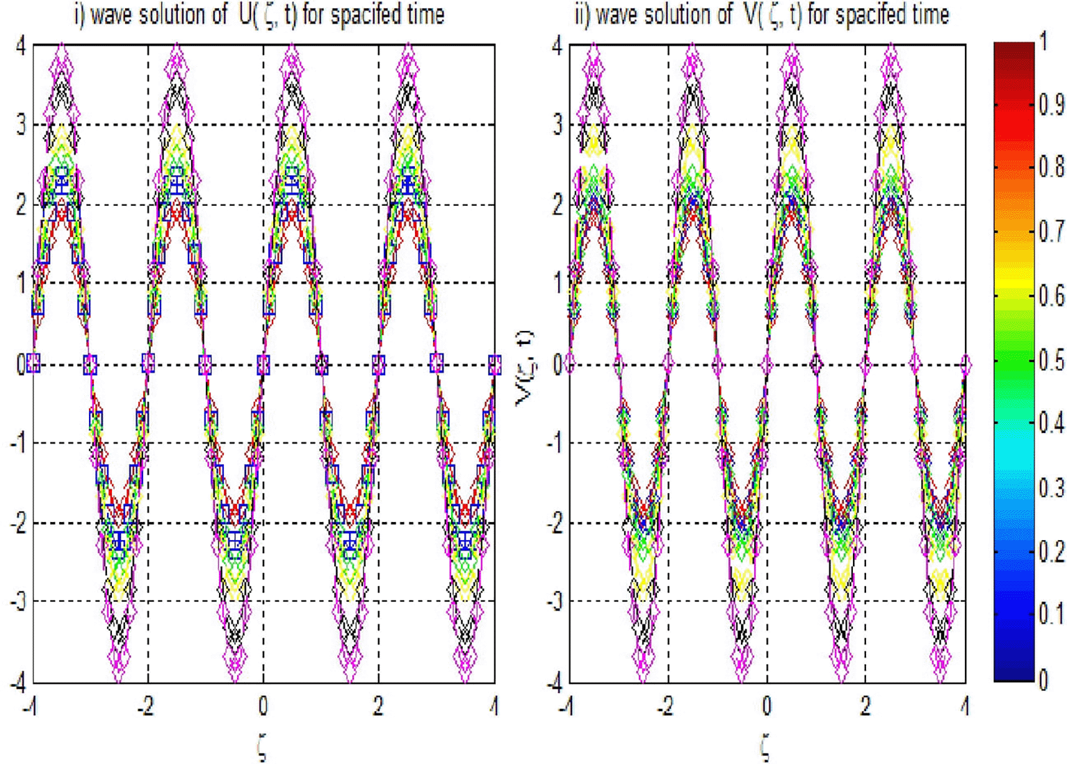
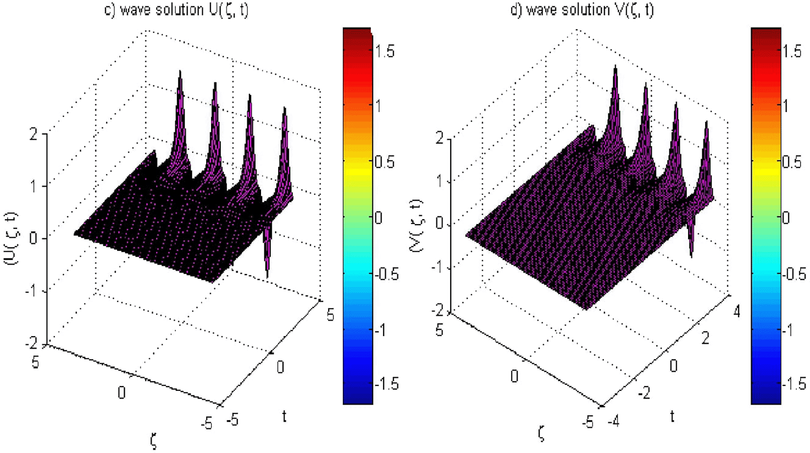
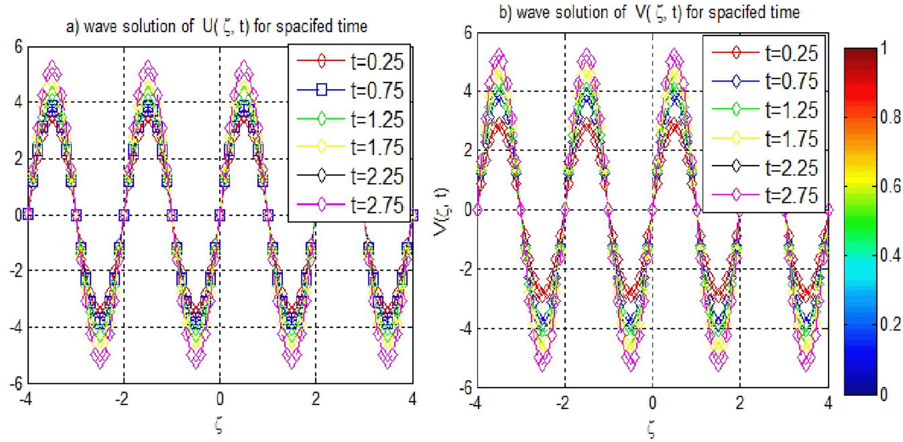
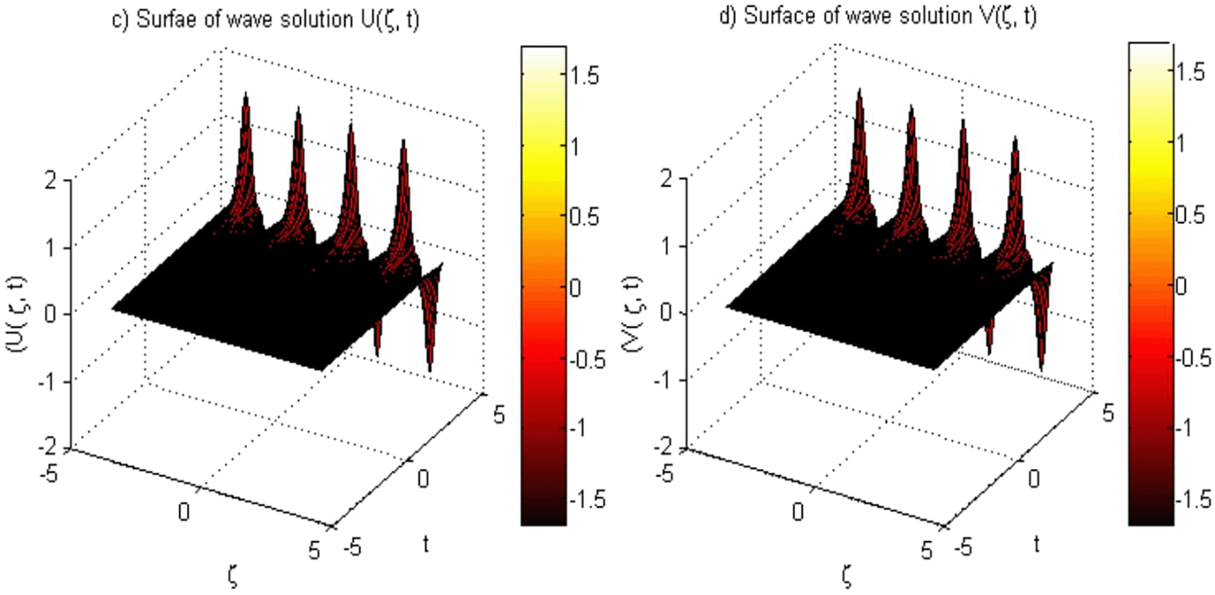
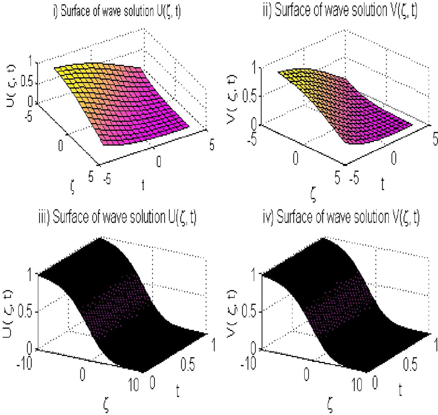
Figures 1 and 2 depict the wave solutions $u (ζ, t)$ and $v (ζ, t)$ , showing stable profiles across varying perturbation parameter $β$ . The convergence of these profiles is consistent with the findings in Table 4, where the $L_{2}$ , $L_{\infty}$ , and Global Relative Error (GRE) values are reported at multiple time levels. Importantly, the numerical solutions approached zero by the 40th time step with a time step size of $Δt = 0.01$ , indicating convergence toward the expected behavior.

Figure 1. Geometric representation of the behavior of wave solution $u (ζ, t)$ and $v (ζ, t)$ with $M = 50$ and $∆ t = 0.01$ for evaluating example one for linear case with $β = 0.002$ .

Figure 2. Geometrical representation of surface of wave solution $u (ζ, t)$ and $v (ζ, t)$ with M = 50 and $∆ t = 0.01$ for Example one for linear case with $β = 0.002$ .

Figure 3. Geometrical representations of behaviors of wave solutions of example one with $β = 10^{- 1},$ $∆ t = 0.01$ and $M = 64$ for linear case.

Figure 4. Geometrical representations of the surface of the wave solution for example one with $β = 10^{- 1},$ $∆ t = 0.01$ and $M = 64$ for linear case.

Figure 5. Geometrical representation of behavior of wave solution $u (ζ, t), v (ζ, t)$ and Surface of error of solution $u (ζ, t),$ for example one with $= 10^{- 4}$ , $∆ t = 0.1$ and $M = 64$ .

Table 4. The Comparisons of $L_{2}$ , $L_{\infty}$ and GRE norm for $∆ t = 0.01$ and $∆ t = 0.001$ for Example one with $M = 64$ for linear case.

Method	Time	$∆ t = 0.01$			$∆ t = 0.001$
Method	Time	$L_{2}$	$L_{\infty}$	$GRN$	$L_{2}$	$L_{\infty}$	$GRN$
Result obtained by present method	$0.0$	0.00	0.00	0.00	0.00	0.00	0.00
	$0.5$	2.14516E−08	6.37461E−07	8.91491E−06	5.47251E−09	4.81836E−07	6.88431E−08
	$1.0$	4.27712E−07	5.81319E−06	8.07116E−06	5.11306E−09	6.48513E−07	5.13658E−08
	$1.5$	5.244112−07	5.14934E−06	7.54718E−06	5.10041E−09	8.11012E−07	5.72458E−08
	$2.0$	5.12876E−07	5.01354E−06	6.93307E−06	4.76766E−09	7.46671E−07	6.53671E−08
	$2.5$	6.20911E−07	4.34211E−06	6.33144E−06	4.00192E−09	4.77169E−07	6.24611E−08
	$3.0$	5.11237E−08	4.27273E−07	4.19635E−06	2.83173E−09	5.92380E−07	6.52783E−07
	$3.5$	7.01785E−08	4.11505E−07	4.00201E−06	2.80059E−09	9.16101E−06	8.59178E−07
	$4.0$	5.26528E−08	3.98151E−07	3.71123E−06	2.29851E−09	8.62193E−06	9.46140E−06
Versus
Results obtained by method in¹⁹	$0.0$	1.42874E−17	8.88178E−16	3.56768E−09	1.42874E−17	8.88178E−16	3.56768E−09
	$0.5$	8.24109E−05	3.12068E−03	5.01495E−03	6.17258E−06	3.92776E−04	5.14833E−04
	$1.0$	4.84202E−05	1.99664E−03	5.05022E−03	2.17706E−06	3.42516E−04	6.00652E−04
	$1.5$	2.76149E−05	1.34984E−03	5.14661E−03	4.41442E−07	3.47012E−04	1.23549E−03
	$2.0$	1.46576E−05	1.01352E−03	5.53307E−03	2.36769E−06	4.06579E−04	3.32529E−03
	$2.5$	6.26190E−06	9.56217E−04	9.09238E−03	4.07361E−06	5.87362E−04	8.69122E−03
	$3.0$	3.44444E−07	1.17377E−03	2.22965E−02	5.93443E−06	9.52380E−04	2.23252E−02
	$3.5$	4.49788E−06	1.65753E−03	5.66291E−02	8.31754E−0	1.53108E−03	5.67165E−02
	$4.0$	9.32854E−06	2.48154E−03	1.42831E−01	1.16591E−05	2.42139E−03	1.43048E−01

Further assessment of spatial discretization is presented in Table 5, demonstrating that reducing the spatial discretization parameter $h$ enhances accuracy, aligning with the theoretical expectations. This confirms that finer discretization contributes to improved precision in numerical solutions across both $Δt = 0.01$ and $Δt = 0.001$ .

Table 5. Comparisons of $L_{2}$ -norm $L \infty$ -norm and GRE for different partitions of the domain of spatial variables and at specified time in the evaluating example one for T = 2 and M = 80.

Time-steps	Norm of error	Results obtained by method in¹⁹				Results obtained by present method
Time-steps	Norm of error	M = 20	M = 40	M = 60	M = 80	M = 20	M = 40	M = 60	M = 80
$∆ t = 0.1$	$L_{2}$	1.37406E−03	4.45938E−04	2.08576E−04	1.19453E−04	2.4581E−06	5.458E−06	4.0857E−07	7.59836E−08
	$L_{\infty}$	8.74229E−03	7.47418E−03	7.10195E−03	6.94779E−03	5.4721E−05	3.748E−06	6.1619E−06	6.94779E−07
	$GRE$	5.28462E−02	5.12724E−02	4.99799E−02	4.99747E−02	6.3846E−04	6.197E−06	6.8478E−06	5.6752E−07
$∆ t = 0.01$	$L_{2}$	1.41692E−04	2.13303E−05	1.60035E−05	7.28243E−05	7.41892E−07	4.634E−06	6.9003E−08	7.28246E−08
	$L_{\infty}$	2.89695E−03	1.47745E−03	1.05749E−03	4.13368E−03	6.89613E−06	4.377E−06	8.2546E−07	5.13368E−07
	$GRE$	1.90780E−02	8.24560E−03	5.62795E−03	5.00313E−03	4.90789E−05	6.945E−05	8.12765E−06	6.00318E−06
$∆ t = 0.001$	$L_{2}$	1.39713E−04	2.12319E−05	3.32691E−06	5.62754E−07	4.97911E−08	7.126E−05	5.62676E−08	7.67758E−09
	$L_{\infty}$	6.28584E−04	8.76524E−04	4.51042E−04	2.87972E−04	7.68685E−07	9.452E−05	6.51042E−06	8.87997E−09
	$GRE$	5.35450E−04	7.92931E−03	3.71863E−03	2.16258E−03	6.81454E−06	9.829E−05	8.71863E−06	5.56257E−07

The results presented in Table 6 highlight the superior performance of the current method in solving the EFK equation, particularly regarding $L_{\infty}$ -norms. Across all time steps and spatial discretizations, the method consistently yields lower error values compared with both approaches in¹⁹ and.³⁹ For instance, with a step size of $Δt = 0.001$ and $h = 1 / 10$ , the current method achieved an $L_{\infty}$ -norm of $1.4193 E - 07$ . This significant improvement in accuracy underscores the effectiveness of the quintic Hermite spline method when paired with Richardson extrapolation, particularly in managing the complexities of boundary value problems.

Table 6. Comparison L ∞-norm of example one at specified time with different step lengths.

Values of T	Step size	By method in³⁹		By Method in¹⁹		By present method
		$L \infty$		$L \infty$		$L \infty$
		$∆ t = 0.01$	$∆ t = 0.001$	$∆ t = 0.01$	$∆ t = 0.001$	$∆ t = 0.01$	$∆ t = 0.001$
T = 1	h = 1/10	7.7195E−2	2.1542E−2	2.5716E−03	9.59093E−04	3.6717E−06	1.4193E−07
	h = 1/20	2.1536R−2	5.8138E−3	2.57163E−03	5.45979E−04	3.6716E−05	6.7596E−07
	h = 1/40	5.8078E−3	1.4625E−3	2.01533E−03	3.62735E−04	4.51317E−5	6.0271E−07
	h = 1/80	1.4567E−3	3.6573E−4	1.94303E−03	2.88109E−04	5.44673E−05	5.1826E−08
T = 2	h = 1/2	2.8445E−2	2.8442E−3	2.89695E−03	6.28584E−04	5.31696E−06	6.2837E−07
	h = 1/5	7.9425E−3	7.9380E−4	1.47745E−03	8.76524E−04	7.46142E−06	3.16614E−07
	h= 1/7.5	2.1437E−3	2.1386E−4	1.05749E−03	4.51042E−04	2.85711E−06	5.58191E−07
	h = 1/10	5.3904E−4	5.3377E−5	4.13368E−03	2.87972E−04	3.13364E−06	1.67976E−07

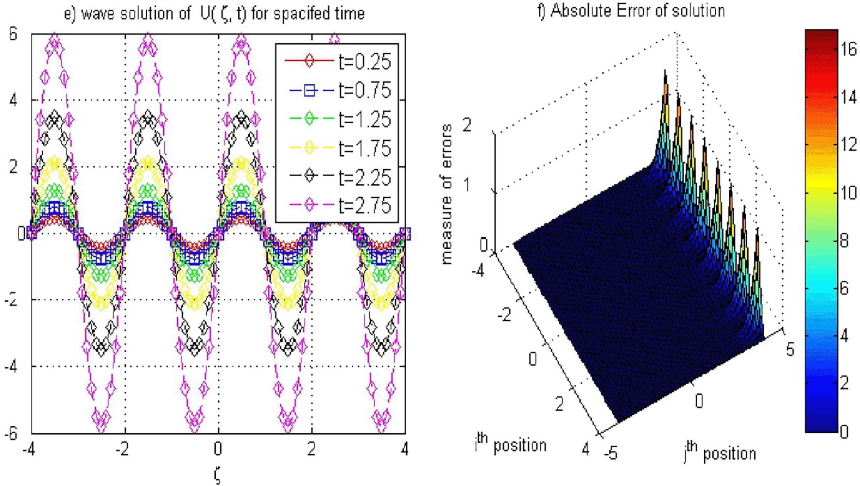
Table 7 further emphasizes the advantages of the current method by comparing absolute errors at various spatial points $(ζ) .$ The errors obtained using this method are consistently lower than those from method,¹⁹ particularly at $t = 0.5$ , where the present method yields an error of $1.12575 E - 06$ versus $1.88514 E - 04$ from method.¹⁹ This demonstrates the method’s robustness in maintaining precision across different spatial coordinates. Furthermore, as demonstrated in Figures 3-4 and 5(f ), the solution for Example 1 is accurately approximated, with Figure 5(e) illustrating the stability of our method at the specified grid points and confirming this accuracy. Overall, the results reinforce the current method’s effectiveness in capturing the dynamics of the EFK equation, showcasing its capability to achieve high accuracy and stability in complex simulations.

Table 7. Comparison of absolute error at different values of $ζ$ in solving example one with $∆ t = 0.01$ and M = 64.

By present method
t	ζ = −3	ζ = −2	ζ = −1	ζ = 0	ζ = 1	ζ = 2	ζ = 3
0.5	1.94262E−05	2.98467E−05	6.88514E−06	1.12575E−06	2.13925E−05	3.30463E−05	2.30463E−05
1.5	4.79342E−06	5.33524E−06	2.51033E−06	5.79580E−06	7.54182E−05	1.00450E−06	8.00550E−05
2.5	7.41854E−05	3.64116E−06	2.05935E−06	6.13465E−05	1.13573E−05	6.25200E−06	1.25400E−05
3.0	5.54962E−05	7.60480E−06	5.51924E−06	5.79554E−05	4.40134E−05	8.21818E−06	6.21814E−06
By method in¹⁹
0.5	2.13925E−03	3.11837E−03	2.30463E−03	1.88514E−04	1.98467E−03	2.94162E−03	2.12575E−03
1.5	8.54182E−04	1.26644E−03	1.00450E−03	2.51032E−04	5.33624E−04	8.79348E−04	5.79580E−04
2.5	4.13573E−04	6.50847E−04	6.25200E−04	4.05935E−04	1.64116E−04	7.41854E−05	2.13465E−04
3.0	3.40134E−04	5.65588E−04	6.21818E−04	5.51928E−04	4.60480E−04	4.53962E−04	5.79854E−04

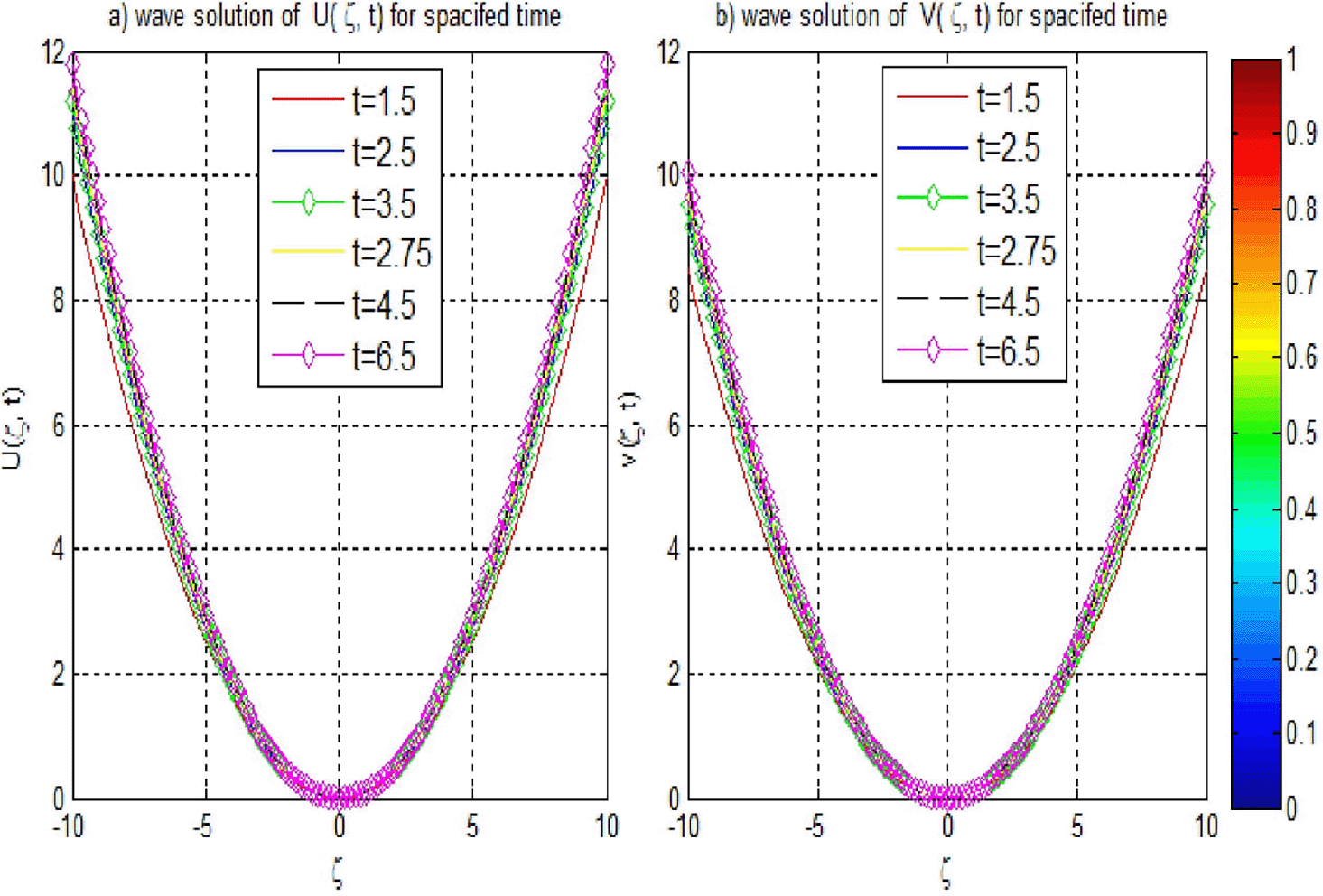
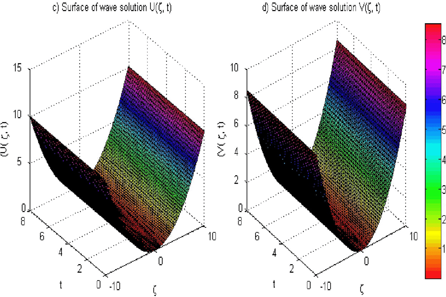
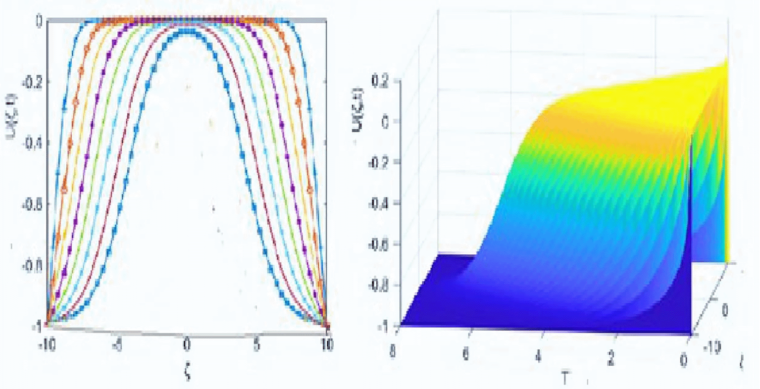
Example 2 examines the numerical results from two cases: (i) with parameters $Δt = 0.01, N = 50$ , and $β = 0.0001$ , and (ii) with $Δt = 0.01, N = 64$ , and $β = 0.01$ . Table 8 reveals that our method consistently achieves lower error values than those in.¹⁹ For instance, at $t = 5$ in the domain $[- 4, 4],$ the $L_{2}$ -norm for our method is $3.6693 E - 03$ , which is significantly better than $1.34938 E - 01$ from the previous method. This illustrates the effectiveness of our approach in capturing the solution behavior and convergence toward a stable boundary value of 1. Additionally, the results in Table 9 show that in case (ii), our proposed method consistently produces lower error norms compared to,¹⁹ with the L2-norm at t = 5 in [-4,4] being 3.6695E−03, much better than 1.3494E−01. The graphical representations in Figures 6 and 7 further elucidate this behavior, showing the evolution of solutions over time and a smooth transition toward stability. Also, Figure 8 further confirms that the solution for Example 2 in case (ii) is well-approximated, suggesting that our approach is more accurate than existing methods.

Table 8. Comparisons of the effects of the current method using the norms in the specified domain for solving example two (i) with $∆ t = 0.01$ and M = 50 and $β = 0.0001$ .

By method in¹⁹					By present method
t	$Ω = [- 4, 4]$		$Ω = [- 10, 10]$		$Ω = [- 4, 4]$		$Ω = [- 10, 10]$
t	$L_{2}$	$L_{\infty}$	$L_{2}$	$L_{\infty}$	$L_{2}$	$L_{\infty}$	$L_{2}$	$L_{\infty}$
0	5.62590E−02	9.96992E−01	1.40648E−01	9.96992E−01	5.1668E−04	7.96992E−03	4.96992E−03	7.62590E−03
1	1.28174E−01	9.55642E−01	2.93265E−01	8.68283E−01	4.9364E−04	8.68283E−03	5.35647E−03	6.28774E−03
2	1.32535E−01	9.80254E−01	3.21779E−01	9.51480E−01	4.21779E−04	6.51481E−03	2.80254E−03	7.32598E−03
3	1.34241E−01	9.93923E−01	3.32150E−01	9.82345E−01	4.36150E−03	4.86345E−03	5.93926E−02	7.34649E−03
4	1.34822E−01	9.98877E−01	3.35790E−01	9.94613E−01	5.75790E−03	8.96616E−03	5.98177E−02	5.34822E−02
5	1.34938E−01	9.99848E−01	3.36935E−01	9.98470E−01	3.66935E−03	1.97470E−02	5.99547E−02	6.34936E−02

Table 9. Comparisons of the effects of the current method using the norms in the specified domain for solving example two (ii) with $∆ t = 0.01$ and M = 64 and $β = 0.01$ .

By method in¹⁹					By present method
t	$Ω = [- 4, 4]$		$Ω = [- 10, 10]$		$Ω = [- 4, 4]$		$Ω = [- 10, 10]$
t	$L_{2}$	$L_{\infty}$	$L_{2}$	$L_{\infty}$	$L_{2}$	$L_{\infty}$	$L_{2}$	$L_{\infty}$
0	4.39524E−02	9.96992E−01	1.09881E−01	9.96992E−01	9.59093E−04	4.634E−03	2.4581E−05	5.1668E−04
1	1.03420E−01	9.48203E−01	2.38273E−01	9.27997E−01	5.45979E−04	4.377E−03	5.4721E−05	4.9364E−04
2	1.03640E−01	9.81968E−01	2.55112E−01	9.85379E−01	3.62735E−04	6.945E−03	6.3846E−04	4.21779E−04
3	1.04187E−01	1.00231E+00	2.60960E−01	9.98986E−01	2.88109E−04	7.126E−03	7.4189E−04	4.36150E−03
4	1.04572E−01	1.00737E+00	2.62897E−01	1.00066E+00	6.28584E−04	9.452E−03	6.8961E−04	5.75790E−03
5	1.04813E−01	1.00650E+00	2.63448E−01	9.99607E−01	8.76524E−04	9.829E−03	4.9789E−04	3.66935E−03

Figure 6. Geometrical representations of behavior of solution $u (ζ, t)$ , $v (ζ, t)$ of example two (i) with Gaussian initial function, $∆ t$ $= 0.01$ and $M = 50$ and $β = 10^{- 1}$ .

Figure 7. Geometrical representations of behavior surface of solution $u (ζ, t)$ , $v (ζ, t)$ of example two (i) with Gaussian initial function, $∆ t$ $= 0.01$ and $M = 50$ and $β = 10^{- 1} .$

Figure 8. Geometrical representations of behavior of solution $u (ζ, t)$ and its surface of example two (ii) with $∆ t = 0.01$ and M = 64 and $β = 0.01$ .

Example 3 reinforces the accuracy of the proposed method, as indicated in Table 10, where the $L_{2} -$ norm at $t = 1$ for the domain $[- 4, 4]$ is $6.37461 E - 05$ , which is markedly lower than $3.50404 E - 02$ from.¹⁹ This method also demonstrates consistently low error values across a larger domain $[- 10, 10]$ indicating robust performance in capturing solution dynamics. Figure 9 visually represents the stability and smoothness of the profiles generated by the proposed method, reinforcing the numerical findings.

Table 10. Comparisons of $L_{2}$ -norm and $L_{\infty}$ -norm in the evaluating example three with $∆ t = 0.01$ and $M = 64$ and $β = 0.01$ .

By present method
t	$Ω = [- 4, 4]$		$Ω = [- 10, 10]$		$Ω = [- 10, 10]$
t	$L_{2}$	$L_{\infty}$	$L_{2}$	$L_{\infty}$	$L_{2}$	$L_{\infty}$
1	6.37461E−05	2.31652E−04	3.76798E−05	1.39465E−04	5.78486E−04	5.039981E−03
2	5.81319E−05	3.86613E−04	6.66779E−04	5.67131E−04	6.186164E−04	5.32188E−03
3	5.14934E−04	3.87335E−04	6.86142E−04	6.77863E−04	6.70266E−04	5.43851E−03
4	5.01354E−04	3.98226E−04	7.87916E−04	7.985288E−4	6.984334E−4	4.7219E−03
5	4.34211E−04	4. 2354E−04	5.65871E−04	4.88919E−03	7.02551E−04	3.6421E−03
By method in¹⁹
1	3.50404E−02	9.31452E−01	2.32795E−03	9.89406E−01	3.48395E−10	9.99968E−01
2	8.60787E−02	9.84613E−01	4.66779E−02	9.96130E−01	1.37028E−08	9.99973E−01
3	1.01901E−01	9.95334E−01	1.74040E−01	9.97860E−01	7.79145E−07	9.99982E−01
4	1.04762E−01	9.98226E−01	2.37816E−01	9.98421E−0	4.49760E−05	9.99989E−01
5	1.05277E−01	9.99239E−01	2.55671E−01	9.98918E−01	2.25922E−03	9.99993E−01

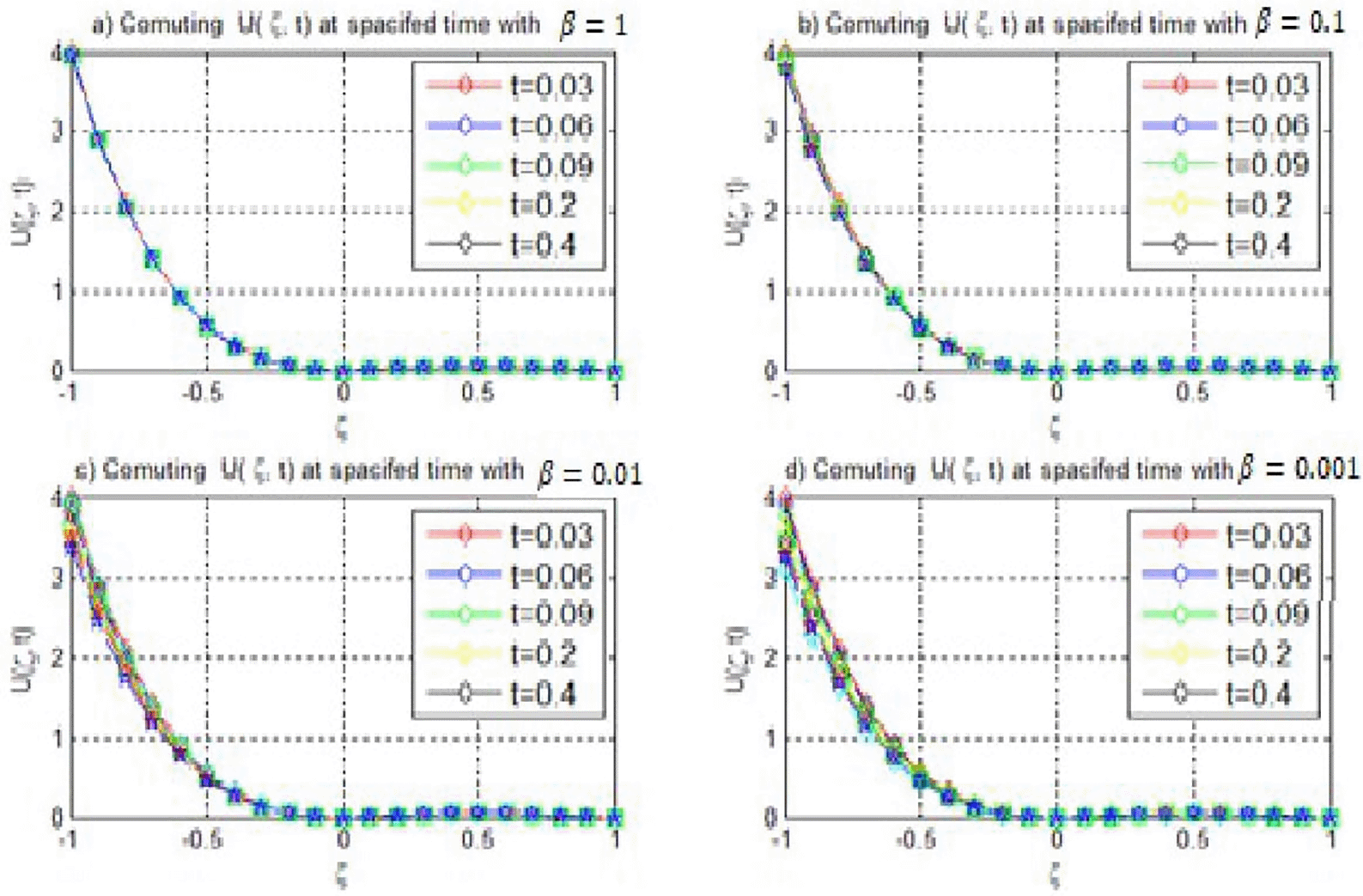
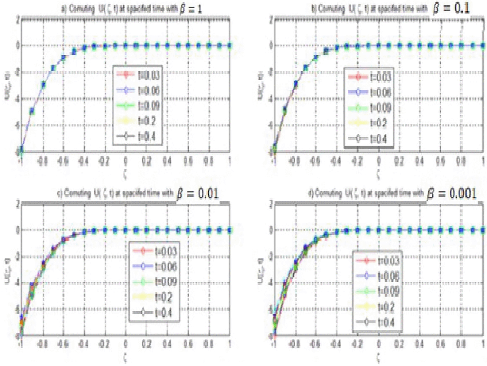
Figure 9. Geometrical representation of the behavior of the solutions $u (ζ, t)$ and $v (ζ, t)$ of Example three for $β = 1$ in different domains with different step-lengths h.

Example 4 presents the results in Table 11, which highlight the significant accuracy improvements with our method. For $t = 0.03$ and $β = 1$ , the $L_{2} -$ norm is $9.1479 E - 07$ , which is significantly lower than the 1.02705E−05 from.¹⁹ The convergence characteristics are further illustrated in Table 12, which reveal superior convergence rates, particularly for finer discretizations. Figures 10 and 11 visually reinforce these numerical findings, displaying the wave solutions $u (ζ, t)$ for different perturbation parameters.

Table 11. Comparisons of $L_{2}$ -norm and $L_{\infty}$ -norm with $∆ t = 0.01$ and M = 50 in the evacuating example 4 (i) with different perturbation parameter $β .$

By present method
t	$β = 1$		$β = 0.001$
t	$L_{2}$	$L_{\infty}$	$L_{2}$	$L_{\infty}$
0.03	9.1479E−07	7.1099E−05	1.63437E−09	5.3561E−07
0.07	2.2991E−08	3.1731E−06	3.59855E−09	2.76467E−07
0.3	6.861E−08	6.1450E−06	4.30266E−09	2.99239E−07
0.7	7.1123E−08	4.8100E−06	4.84632E−09	3.65787E−07
0.9	2.4923E−08	5.3651E−06	5.00983E−10	4.12116E−08
By method in¹⁹
0.03	1.02705E−05	4.03076E−03	8.83277E−06	1.08170E−02
0.07	9.69180E−06	2.67816E−03	7.19451E−06	7.26425E−03
0.3	4.11284E−06	9.31101E−04	8.30286E−07	8.42396E−04
0.7	1.81930E−06	3.07393E−04	1.54302E−08	2.32675E−05
0.9	1.49806E−06	2.36168E−04	2.60093E−09	3.86667E−06

Table 12. Comparisons of parametric-uniform maximum absolute errors and its rate of convergence for $T = 0.04$ in the evaluating example four in case (ii) for $Δ t = 10^{- 3} .$

$β$	By method in¹⁹				By present method
$β$	M = 8	M = 16	M = 32	M = 64	M = 8	M = 16	M = 32	M = 64
$2^{- 0}$	6.41841E−06	3.22272E−06	1.60909E−06	8.03679E−07	1.4684E−06	5.458E−06	3.0857E−07	9.59836E−08
$2^{- 1}$	1.80796E−05	8.98549E−06	4.68089E−06	2.34057E−06	3.4728E−06	3.748E−06	6.1619E−06	8.94779E−07
$2^{- 2}$	0.00010412	0.00005501	2.78666E−05	1.39476E−05	6.3846E−05	6.197E−06	6.7328E−06	3.6752E−07
$2^{- 3}$	6.41841E−06	3.22272E−06	1.60909E−06	8.05E−07	6.41892E−05	4.634E−06	7.9003E−06	4.9441E−07
$2^{- 4}$	8.66285E−05	4.60583E−05	2.31932E−05	1.15962E−05	6.89613E−05	4.377E−06	8.1546E−06	9.13368E−07
$2^{- 6}$	0.00010412	0.00005501	2.78666E−05	1.39476E−05	7.90789E−05	6.945E−05	8.12765E−06	4.11315E−06
$2^{- 8}$	0.00010412	0.00005501	2.78666E−05	1.39476E−05	7.97911E−05	7.126E−05	3.12674E−05	5.17758E−06
$E_{N}$	0.00010412	0.00005501	2.78666E−05	1.39476E−05	8.68685E−05	9.452E−05	4.51042E−05	9.87997E−06
$R_{N}$	0.920481409	0.981156913	0.998520095	-	8.81454E−05	9.829E−05	4.75863E−06	1.56257E−03

Table 13. Comparisons of $L_{2}$ -norm and $L_{\infty}$ -norm of error in the evaluating example five for both $∆ t = 0.01$ , $∆ t = 0.001$ and $M = 64$ .

t	By method in¹⁹				By present method
	Time step	$∆ t = 0.01$	$∆ t = 0.001$		$∆ t = 0.01$		$∆ t = 0.001$
	$L_{2}$	$L_{\infty}$	$L_{2}$	$L_{\infty}$	$L_{2}$	$L_{\infty}$	$L_{2}$	$L_{\infty}$
0.1	8.56447E−06	1.06174E−03	8.33926E−06	1.14140E−03	4.59093E−07	5.634E−05	8.4581E−07	9.1668E−06
0.2	1.13259E−05	1.80386E−03	1.11443E−05	1.87280E−03	8.45979E−07	6.377E−05	9.8721E−07	2.9364E−06
0.4	1.54954E−05	3.07668E−03	1.54042E−05	3.13596E−03	2.12735E−06	9.945E−05	3.6843E−06	1.7179E−05
0.6	1.91941E−05	4.16207E−03	1.91346E−05	4.21119E−03	4.78109E−06	2.126E−04	3.4188E−06	5.36150E−05
0.8	2.23256E−05	5.04855E−03	2.22705E−05	5.08817E−03	4.28582E−06	2.452E−04	4.0061E−06	6.75790E−05
1.0	2.46120E−05	5.78314E−03	2.47896E−05	5.78346E−03	6.16524E−06	3.829E−04	4.2389E−06	6.12935E−05

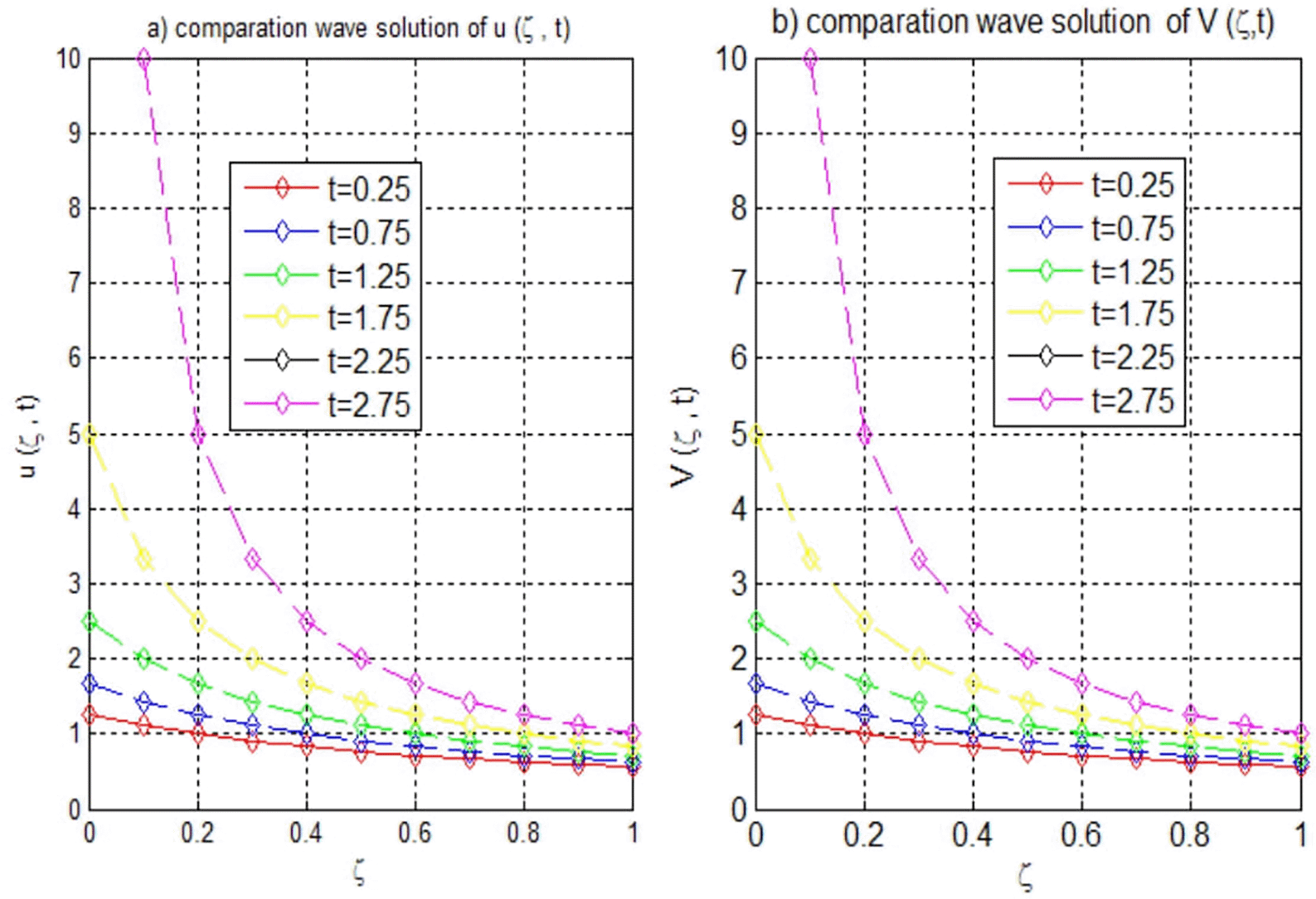
Figure 10. Geometrical comparison of wave solution $u (ζ, t)$ of example 4(i) for different perturbation parameter $β$ and $M = 32$ .

Figure 11. Geometrical comparison of wave solution $u (ζ, t),$ of example four (ii) with different perturbation parameter $β$ and $M = 40$ .

Example 5 illustrates the effectiveness of the proposed method in achieving lower error norms across various time steps and sizes. As it is showing in Table 13, at t = 0.1 with Δt = 0.01, the $L_{2} -$ norm was $4.5909 E - 07$ , which was substantially lower than $8.56447 E - 06$ from.¹⁹ The results in Table 14 confirm that our method consistently yields lower $L_{2}$ and $L_{\infty} -$ norms, particularly with finer time steps, demonstrating stability and robustness in simulating wave solutions. Also as it is shown in Table 15, the present method significantly reduces the maximum absolute errors compared to the method in,¹⁹ especially as M increases, demonstrating faster convergence. The errors decrease by several orders of magnitude across all parameters, indicating the superior accuracy and efficiency of the proposed approach. Based on this results, the present method outperforms the previous method in both accuracy and convergence rate. Figures 12 and 13 visually represent the behavior of the wave solutions $u (ζ, t)$ and $v (ζ, t)$ affirming the numerical findings.

Table 14. Comparison of $L_{2}$ -norm, $L_{\infty}$ -norm and GRE in the evaluating example five in the time interval 0 < t ≤ 0.5.

Time-steps	Norm of error	Results obtained by method in¹⁹				Results obtained by present method
Time-steps	Norm of error	M = 20	M = 40	M = 60	M = 80	M = 20	M = 40	M = 60	M = 80
$∆ t = 0.1$	$L_{2}$	2.69111E−04	3.41167E−05	1.20233E−05	6.11513E−06	3.51E−06	5.458E−06	4.857E−07	7.598E−07
	$L_{\infty}$	5.88431E−03	3.91978E−03	3.59510E−03	3.48590E−03	4.72E−05	2.74E−06	5.619E−06	4.949E−07
	$GRN$	5.37349E−02	3.58310E−02	3.25095E−02	3.13709E−02	4.84E−04	5.197E−06	6.547E−05	3.62E−05
$∆ t = 0.01$	$L_{2}$	2.38562E−04	3.04466e−05	1.09433E−05	5.63647E−06	5.48E−07	3.637E−06	2.263E−08	2.246E−08
	$L_{\infty}$	5.93525E−03	3.91185E−03	3.58612E−03	3.47732E−03	6.93E−06	3.375E−06	5.254E−07	5.118E−07
	$GRN$	5.36526E−02	3.57576E−02	3.24471E−02	3.13131E−02	4.99E−05	5.445E−05	8.276E−06	6.31E−06
$∆ t = 0.001$	$L_{2}$	2.3968E−04	3.0887E−05	1.11036E−05	5.7122E−06	5.97E−08	6.726E−05	5.6676E−07	4.332E−07
	$L_{\infty}$	5.9765E−03	3.9128E−03	3.58625E−03	3.4778E−03	6.68E−07	7.452E−05	5.5104E−07	3.877E−07
	$GRN$	5.3665E−02	3.5729E−02	3.24500E−02	3.1351E−02	6.45E−06	8.829E−05	6.713E−06	7.562E−06

Table 15. Comparisons of parameter-uniform maximum absolute errors and its rate of convergence in the evaluating example five in the time interval 0 < t ≤ 0.2.

By present method
$β$	M = 5	M = 10	M = 20	M = 40	M = 80
$2^{0}$	$3.113 E - 4$	$2.9925 E - 4$	$1.925 E - 4$	$2.25 E - 4$	$5.78133 E - 5$
$2^{- 1}$	$3.811 e - 4$	$2.9987 E - 4$	$1.875 E - 4$	$3.657 E - 4$	$6.39984 E - 4$
$2^{- 2}$	$4.834 E - 3$	$2.8023 E - 4$	$1.023 E - 4$	$3.373 E - 4$	$6.83074 E - 4$
$2^{- 3}$	$4.835 E - 3$	$8.1703 E - 3$	$1.173 E - 4$	$4.108 E - 4$	$6.97700 E - 4$
$2^{- 4}$	$5.837 E - 3$	$1.6629 E - 3$	$1.629 E - 4$	$4.629 E - 4$	$7.6629 E - 4$
$2^{- 5}$	$5.847 E - 3$	$4.0241 E - 3$	$1.041 E - 4$	$4.841 E - 4$	$7.8241 E - 4$
$E_{N}$	$7.315 E - 3$	$8.9243 E - 3$	$1.943 E - 4$	$5.923 E - 4$	$7.9243 E - 4$
$R_{N}$	$1.26113 E - 3$	$1.1375 E - 3$	$2.1375 E - 4$	$5.985 E - 4$	$8.1375 E - 4$
By method in¹⁹
$2^{0}$	0.027097829	0.006278871	0.001656379	0.000414531	0.000103733
$2^{- 1}$	0.04799501	0.016872231	0.004031238	0.001016282	0.000255155
$2^{- 2}$	0.045440459	0.024649882	0.007400184	0.001811592	0.000454294
$2^{- 3}$	0.045353053	0.025807968	0.008589973	0.002413281	0.000038522
$2^{- 4}$	0.045512133	0.025971564	0.008671138	0.002484271	0.000689575
$2^{- 5}$	0.045528756	0.025983209	0.008669169	0.002492881	0.000685876
$E_{N}$	0.04799501	0.025983209	0.008671138	0.002492881	0.000689575
$R_{N}$	0.885304799	1.583286368	1.798407329	1.854034639	-

Figure 12. Geometrical comparison of wave solution $u (ζ, t)$ and $v (ζ, t)$ of example five using different step-length $h$ and at specified time with $∆ t = 0.01 .$

Figure 13. Geometrical representation of the behavior solution $u (ζ, t)$ and $v (ζ, t)$ of example five for $β = 1$ and M = 20.

Finally, Example 6 examines the effects of varying α, with $β = 1$ . For $α = 1$ , as listed in Table 16, our method achieved lower error norms across the perturbation parameters. Conversely in Table 17, for $α = - 1$ , while the method still performs favorably, the error norms are generally higher, indicating an increased sensitivity to perturbations. Figures 14–16 visually represent the evolution of wave solutions for both $α = 1$ and $α = - 1$ , highlighting the stability of our method in the positive alpha scenario.

Table 16. Comparisons of $L_{2}$ -norm and $L_{\infty}$ -norm in the evaluating example six for $∆ t = 0.01$ and M = 32, with $α = 1$ .

By present method
t	$β = 1$		$β = 0.1$		$β = 0.001$
t	$L_{2}$	$L_{\infty}$	$L_{2}$	$L_{\infty}$	$L_{2}$	$L_{\infty}$
0.1	6.97298E−05	4.96037E−04	4.17722E−05	7.97298E−03	7.17873E−04	3.98307E−03
0.2	5.55890E−04	3.53767E−03	4.27609E−04	4.55890E−03	7.98819E−04	4.57292E−03
0.4	5.66262E−04	3.46375E−03	2.36105E−04	4.50262E−03	6.36350E−03	6.07897E−02
0.6	5.48152E−04	3.45341E−03	2.43169E−03	3.48152E−03	6.43448E−03	6.50014E−02
0.8	5.82118E−04	3.79042E−03	3.48896E−03	3.82118e−03	6.49206E−03	4.84189E−01
0.9	5.96414E−04	4.93220E−03	1.51306E−03	3.96414E−03	6.51630E−03	4.98581E−01
By method in¹⁹
0.1	1.72000E−02	6.51753E−01	1.70980E−02	6.47390E−01	1.69815E−02	6.42528E−01
0.2	1.69010E−02	6.40410E−01	1.67894E−02	6.35634E−01	1.66406E−02	6.29654E−01
0.4	1.62911E−02	6.17275E−01	1.61859E−02	6.12772E−01	1.60308E−02	6.06588E−01
0.6	1.56667E−02	5.93590E−01	1.55692E−02	5.89418E−01	1.54229E−02	5.83585E−01
0.8	1.50302E−02	5.69451E−01	1.49402E−02	5.65600E−01	1.48039E−02	5.60161E−01
0.9	1.47083E−02	5.57246E−01	1.46220E−02	5.53549E−01	1.44906E−02	5.48306E−01

Table 17. Comparison of $L_{2}$ -norm and $L_{\infty}$ -norm in the evaluating example six with $∆ t = 0.01$ and M = 32, α = -1.

By present method
t	$β = 1$		$β = 0.1$		$β = 0.001$
t	$L_{2}$	$L_{\infty}$	$L_{2}$	$L_{\infty}$	$L_{2}$	$L_{\infty}$
0.1	3.59093E−04	2.59093E−03	4.59093E−04	4.59093E−04	5.59093E−03	1.59093E−03
0.2	4.15979E−03	3.45979E−03	3.45979E−04	5.45979E−03	4.45979E−03	1.45979E−02
0.4	4.32735E−03	2.12735E−03	3.32735E−03	2.12735E−03	4.12735E−03	2.12735E−02
0.6	4.78109E−03	4.18109E−03	4.74109E−03	4.78109E−03	3.78109E−03	2.78109E−02
0.8	5.28582E−03	4.28582E−02	5.28582E−03	4.28582E−03	3.28582E−03	2.28582E−02
0.9	5.16524E−03	6.16524E−02	5.191524E−03	6.64324E−03	3.26524E−03	3.16524E−02
By method in¹⁹
0.1	1.17873E−02	6.98307E−01	1.17722E−02	6.97298E−01	1.17533E−02	6.96037E−01
0.3	1.27819E−02	7.57292E−01	1.27609E−02	7.55890E−01	1.27291E−02	7.53767E−01
0.5	1.36350E−02	8.07897E−01	1.36105E−02	8.06262E−01	1.35729E−02	8.03753E−01
0.7	1.43448E−02	8.50014E−01	1.43169E−02	8.48152E−01	1.42747E−02	8.45341E−01
0.9	1.49206E−02	8.84189E−01	1.48896E−02	8.82118E−01	1.48435E−02	8.79042E−01
1.0	1.51630E−02	8.98581E−01	1.51306E−02	8.96414E−01	.50827E−02	8.93220E−01

Figure 14. Geometrically the of solution $u (ζ, t)$ and $v (ζ, t)$ of example six for $∆ t = 0.01$ , M = 32, $α = 1$ and $β = 1$ .

Figure 15. Geometrical comparison of wave solution $(ζ, t)$ and $v (ζ, t),$ of example 6 for $∆ t = 0.01$ , M = 32, $α = - 1$ and $β = 1$ .

Figure 16. Geometrical representation of surfaces of solution $u (ζ, t)$ and $u (ζ, t)$ for $∆ t = 0.01$ , M = 32, $α = - 1$ and $β = 1$ .

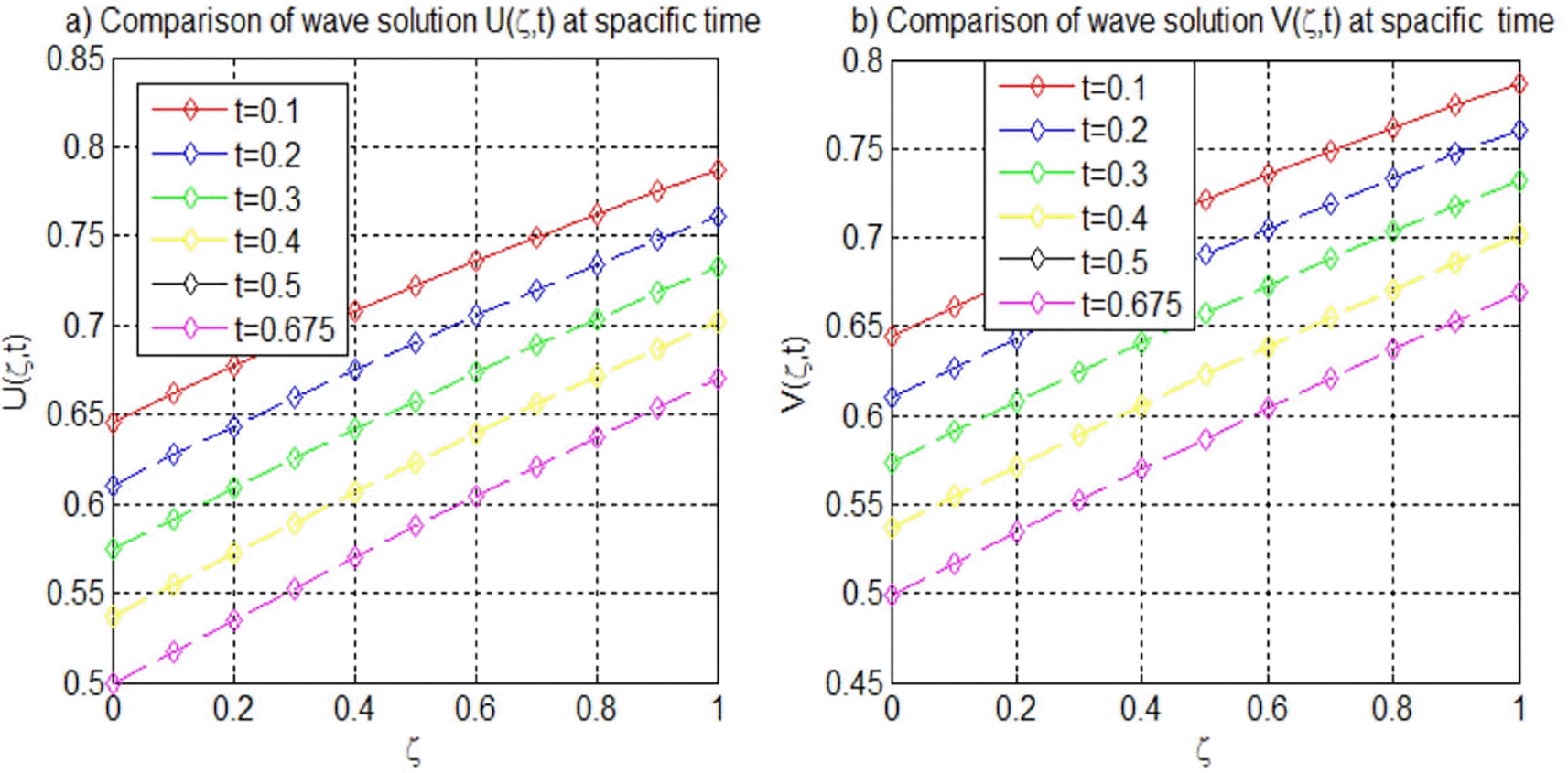
Overall, the application of the Richardson extrapolation technique significantly enhanced the accuracy and convergence of our proposed method, demonstrating its robustness across various EFK-type equations and conditions.

7. Conclusions

This paper presents an advanced numerical method designed to solve the fourth-order Fisher-Kolmogorov reaction-diffusion equation utilizing a hybrid approach that combines quintic Hermite splines with Richardson extrapolation. This innovative technique demonstrates substantial improvements in both accuracy and stability compared with traditional numerical methods. By leveraging the properties of quintic Hermite splines, the proposed method achieves high-order convergence, specifically sixth-order convergence in the spatial direction and fourth-order convergence in the temporal direction. This level of precision is crucial for accurately modeling the complex nonlinear dynamics that are often encountered in various scientific fields.

A thorough stability analysis underscores the capability of the method to maintain unconditional stability across different perturbation parameters, thereby ensuring that the numerical solutions remain bounded and reliable. This aspect of stability is vital, particularly in applications involving dynamic systems where small errors can propagate and lead to significant inaccuracies. The numerical experiments conducted in this study further validate the effectiveness of the proposed method. These experiments demonstrate that it consistently yields lower error norms than existing techniques, highlighting its robustness in capturing the behavior of wave solutions under various initial and boundary conditions.

In addition to its methodological contributions, this research emphasizes the relevance of the proposed technique in mathematical biology and ecology, where the accurate modeling of dynamic processes is essential. These findings illustrate how advanced numerical approaches can enhance our understanding of complex systems, ultimately providing valuable tools for researchers in these fields. Overall, this study represents a significant advancement in numerical analysis for challenging differential equations, showcasing the potential of innovative methodologies to improve the solution reliability and accuracy in scientific computing.

Data availability statement

This study contains all of the data and materials used for conducting this research. This means that all of the data and materials supporting the results or analyses are available within this study.

Acknowledgements

This work was supported by help and encouragement from friends and colleagues. I extend my gratitude for the invaluable insights provided during my research. Thank you to all those who contributed to the successful completion of this work.

References

1. Rajan MP, Reddy GD: A generalized regularization scheme for solving singularly Perturbed parabolic PDEs. Partial Differential Equations in Applied Mathematics. 2022; 5: 100270. Publisher Full Text
2. Rottschäfer V: Multi-bump patterns by a normal form approach. Discrete and Continuous Dynamical Systems-B. 2001; 1(3): 363–386. Publisher Full Text
3. Jaiswal S, Chopra M, Das S: Numerical solution of non-linear partial differential equation for porous media using operational matrices. Math. Comput. Simul. 2019; 160: 138–154. Publisher Full Text
4. Abo-Dahab SM, Abdelhafez MA, Mebarek-Oudina F, et al.: MHD Casson nanofluid flow over nonlinearly heated porous medium in presence of extending surface effect with Suction/injection. Indian Journal of Physics. 2021; 95(12): 2703–2717. Publisher Full Text
5. Rohila R, Mittal RC: A numerical study of two-dimensional coupled systems and higher order partial differential equations. Asian-European Journal of Mathematics. 2019; 12(05): 1950071. Publisher Full Text
6. Mebarek-Oudina F: Convective heat transfer of Titania nanofluids of different base fluids in a cylindrical annulus with a discrete heat source. Heat Transfer—Asian Research. 2019; 48(1): 135–147. Publisher Full Text
7. Clark V, Meyer JC: On two-signed solutions to a second order semi-linear parabolic partial differential equation with non-Lipschitz nonlinearity. J. Differ. Equ. 2020; 269(2): 1401–1431. Publisher Full Text
8. Abbasbandy S, Asady B: Newton’s method for solving fuzzy nonlinear equations. Appl. Math. Comput. 2004; 159(2): 349–356. Publisher Full Text
9. Arora U, Karaa S, Mohanty RK: A new stable variable mesh method for 1-D non-linear parabolic partial differential equations. Appl. Math. Comput. 2006; 181(2): 1423–1430. Publisher Full Text
10. Dehghan M, Hooshyarfarzin B, Abbaszadeh M: Numerical simulation based on a combination of finite-element method and proper orthogonal decomposition to prevent groundwater contamination. Eng. Comput. 2022; 38(4): 3445–3461. Publisher Full Text
11. Wang J, Li H, He S, et al.: A new linearized Crank–Nicolson mixed element scheme for the extended Fisher–Kolmogorov equation. Sci. World J. 2013; 2013(1): 756281. PubMed Abstract | Publisher Full Text | Free Full Text
12. Samir I, Badra N, Seadawy AR, et al.: Exact wave solutions of the fourth order non-linear partial differential equation of optical fiber pulses using different methods. Optik. 2021; 230: 166313. Publisher Full Text
13. Knibb D, Scraton RE: A collocation method for the numerical solution of non-linear parabolic partial differential equations. IMA J. Appl. Math. 1978; 22(3): 305–315. Publisher Full Text
14. Abbasbandy S: Numerical solution of non-linear Klein–Gordon equations by variational iteration method. Int. J. Numer. Methods Eng. 2007; 70(7): 876–881. Publisher Full Text
15. Gavete L, Ureña F, Benito JJ, et al.: Solving second order nonlinear elliptic partial differential equations using generalized finite difference method. J. Comput. Appl. Math. 2017; Vol. 318: pp. 378–387. Publisher Full Text
16. Mansour MBA: Traveling wave patterns in nonlinear reaction–diffusion equations. J. Math. Chem. 2010; 48(3): 558–565. Publisher Full Text
17. Zhou Q, Ekici M, Sonmezoglu A, et al.: Exact solitary wave solutions to the generalized Fisher equation. Optik. 2016; 127(24): 12085–12092. Publisher Full Text
18. Belmonte-Beitia J, Calvo GF, Perez-Garcia VM: Effective particle methods for Fisher–Kolmogorov equations: theory and applications to brain tumor dynamics. Commun. Nonlinear Sci. Numer. Simul. 2014; 19(9): 3267–3283. Publisher Full Text
19. Priyanka P, Mebarek-Oudina F, Sahani S, et al.: Travelling wave solution of fourth order reaction diffusion equation using hybrid Quintic hermite splines collocation technique. Arab. J. Math. 2024; 13(2): 1–27.
20. Fisher RA: The wave of advance of advantageous genes. Ann. Eugenics. 1937; 7(4): 355–369. Publisher Full Text
21. Aronson DG, Weinberger HF: Multidimensional nonlinear diffusion arising in population genetics. Adv. Math. 1978; 30(1): 33–76. Publisher Full Text
22. Dee GT, Van Saarloos W: Bistable systems with propagating fronts leading to pattern Formation. Phys. Rev. Lett. 1988; 60(25): 2641–2644. PubMed Abstract | Publisher Full Text
23. Van Saarloos W: Dynamical velocity selection: marginal stability. Phys. Rev. Lett. 1987; 58(24): 2571–2574. PubMed Abstract | Publisher Full Text
24. Coullet P, Elphick C, Repaux D: Nature of spatial chaos. Phys. Rev. Lett. 1987; 58(5): 431–434. Publisher Full Text
25. Field RJ: Oscillations and Traveling Waves in Chemical Systems. Field RJ, Burger M: New York: Wiley-Interscience; 1985; 95. .
26. Hornreich RM, Luban M, Shtrikman S: Critical behavior at the onset of k-space instability on the λ line. Phys. Rev. Lett. 1975; 35(25): 1678–1681. Publisher Full Text
27. Zimmermann W: Propagating fronts near a Lifshitz point. Phys. Rev. Lett. 1991; 66(11): 1546. PubMed Abstract | Publisher Full Text
28. Coullet P, Huerre P: New Trends in Nonlinear Dynamics and Pattern-Forming Phenomena: The Geometry of Nonequilibrium. Springer Science & Business Media; 2012; vol. 237. .
29. Focant S, Gallay T: Existence and stability of propagating fronts for an autocatalytic reaction–diffusion system. Physica D: Nonlinear Phenomena. 1998; 120(3–4): 346–368. Publisher Full Text
30. Rottschäfer V, Wayne CE: Existence and stability of traveling fronts in the extended Fisher–Kolmogorov equation. J. Differ. Equ. 2001; 176(2): 532–560. Publisher Full Text
31. Rottschäfer V, Doelman A: On the transition from the Ginzburg–Landau equation to the extended Fisher–Kolmogorov equation. Physica D: Nonlinear Phenomena. 1998; 118(3–4): 261–292. Publisher Full Text
32. Pani AK: Numerical methods for the extended Fisher–Kolmogorov (EFK) equation. Int. J. Numer. Anal. Model. 2006; 3(2): 186–210.
33. Peletier LA, Troy WC: Chaotic spatial patterns described by the extended Fisher–Kolmogorov equation. J. Differ. Equ. 1996; 129(2): 458–508. Publisher Full Text
34. Peletier LA, Troy WC: Spatial patterns described by the extended Fisher–Kolmogorov Equation: periodic solutions. SIAM J. Math. Anal. 1997; 28(6): 1317–1353. Publisher Full Text
35. van den Berg JB : Uniqueness of solutions for the extended Fisher–Kolmogorov equation. Comptes Rendus de l’Académie des Sciences-Series I-Mathematics. 1998; 326(4): 447–452.
36. Peletier LA, Troy WC: Spatial patterns described by the extended Fisher–Kolmogorov (EFK) equation. kinks. 1995; 8(6): 1279–1304.
37. Kalies WD, Kwapisz J, VanderVorst RCAM: Homotopy classes for stable connections between Hamiltonian saddle focus equilibria. Commun. Math. Phys. 1998; 193(2): 337–371. Publisher Full Text
38. Peletier LA, Troy WC: A topological shooting method and the existence of kinks of the extended Fisher–Kolmogorov equation. Topological Methods in Nonlinear Analysis. 1995; 6(2): 331–355. Publisher Full Text
39. Abbaszadeh M, Dehghan M, Khodadadian A, et al.: Error analysis of interpolating element free Galerkin method to solve non-linear extended Fisher–Kolmogorov equation. Comput. Math. Appl. 2020; 80(1): 247–262. Publisher Full Text
40. Danumjaya P, Pani AK: Orthogonal cubic spline collocation method for the extended Fisher–Kolmogorov equation. J. Comput. Appl. Math. 2005; 174(1): 101–117. Publisher Full Text
41. Mittal RC, Dahiya S: A study of quintic B-spline based differential quadrature method for a class of semi-linear Fisher–Kolmogorov equations. Alex. Eng. J. 2016; 55(3): 2893–2899. Publisher Full Text
42. Arora G, Joshi V: Simulation of generalized nonlinear fourth order partial differential equation with quintic trigonometric differential quadrature method. Mathematical Models and Computer Simulations. 2019; 11(6): 1059–1083. Publisher Full Text
43. Danumjaya P, Pani AK: Finite element methods for the extended Fisher–Kolmogorov Equation. Research Report: IMG RR-2002-3. Bombay: Industrial Mathematics Group, Department of Mathematics, IIT; 2002.
44. Gudi T, Gupta HS: A fully discrete C0 interior penalty Galerkin approximation of the extended Fisher–Kolmogorov equation. J. Comput. Appl. Math. 2013; 247: 1–16. Publisher Full Text
45. Kaur D, Mohanty RK: Two-level implicit high ordermethod based on half-step discretization for 1D unsteady biharmonic problems of first kind. Appl. Numer. Math. 2019; 139: 1–14. Publisher Full Text
46. Kudryashov NA: Quasi-exact solutions of the dissipative Kuramoto–Sivashinsky equation. Appl. Math. Comput. 2013; 219(17): 9213–9218. Publisher Full Text
47. Dehghan M, Shafieeabyaneh N: Local radial basis function-finite-difference method to simulate some models in the nonlinear wave phenomena: regularized long-wave and extended Fisher–Kolmogorov equations. Eng. Comput. 2021; 37(2): 1159–1179. Publisher Full Text
48. Arora S, Kaur I, Tilahun W: An exploration of quintic Hermite splines to solve Burgers equation. Arab. J. Math. 2020; 9(1): 19–36.
49. Arora S, Jain R, Kukreja VK: Solution of Benjamin–Bona–Mahony–Burgers equation using collocation method with quintic Hermite splines. Appl. Numer. Math. 2020; 154: 1–16. Publisher Full Text
50. Arora S, Kaur I: An efficient scheme for numerical solution of Burgers? Equation using quintic Hermite interpolating polynomials. The Arabian Journal of Mathematics. 2016; 5(1): 23–34. Publisher Full Text
51. Alba-Fernández V, Ibáñez-Pérez MJ, Jiménez-Gamero MD: A bootstrap algorithm for the two-sample problem usingtrigonometric Hermite spline interpolation. Commun. Nonlinear Sci. Numer. Simul. 2004; 9(2): 275–286. Publisher Full Text
52. Merga FE, Chemeda HM: Modified crank–Nicolson scheme with richardson extrapolation for one-dimensional heat equation. Iranian Journal of Science and Technology Transaction A-Science. 2021; 45: 1725–1734. Publisher Full Text
53. Siraj MK, Duressa GF, Bullo TA: Fourth-order stable central difference with Richardson Extrapolation method for second-order self-adjoint singularly perturbed boundary value problems. Journal of the Egyptian Mathematical Society. 2019; 27: 1–4.
54. Chemeda HM, Negassa AD, Merga FE: Compact finite difference scheme combined with Richardson extrapolation for Fisher’s equation. Math. Probl. Eng. 2022; 2022(1): 7887076.
55. Elliott CM, French DA, Milner FA: A second order splitting method for the Cahn–Hilliard equation. Numer. Math. 1989; 54(5): 575–590. Publisher Full Text
56. Sousa E, Li C: A weighted finite difference method for the fractional diffusion equation based on the Riemann–Liouville derivative. Appl. Numer. Math. 2015; 90: 22–37. Publisher Full Text
57. Bhal SK, Danumjaya P, Fairweather G: The Crank–Nicolson orthogonal spline collocation method for one-dimensional parabolic problems with interfaces. J. Comput. Appl. Math. 2021; 383: 113–119.
58. Arora S, Dhaliwal SS, Kukreja VK: Computationally efficient technique for weight functions and effect of orthogonal polynomials on the average. Appl. Math. Comput. 2007; 186(1): 623–631. Publisher Full Text
59. Majeed A, Kamran M, Abbas M, et al.: An efficient numerical technique for solving time-fractional generalized Fisher’s equation. Front. Phys. 2020; 8: 293. Publisher Full Text
60. Abagero BM, Duressa GF, Debela HG: Singularly perturbed robin type boundary value problems with discontinuous source term in geophysical fluid dynamics. Iranian Journal of Numerical Analysis and Optimization. 2021; 11(2): 351–364.
61. Gaddah WA: A higher-order finite-difference approximation with Richardson’s extrapolation to the energy eigenvalues of the quartic, sextic and octic anharmonic oscillators. Eur. J. Phys. 2015; 36(3): 035025. Publisher Full Text
62. Smith GD: Numerical solution of partial differential equations: finite difference methods. Oxford university press; 1985.
63. Kumar D, Kadalbajoo MK: A parameter-uniform numerical method for time-dependent singularly perturbed ifferentialdifference equations. Appl. Math. Model. 2011; 35(6): 2805–2819. Publisher Full Text
64. Keten A, Duman A, Aydin K: Sensitivity of Hurwitz Stability of Linear Differential Equation Systems with Periodic Coefficients. Konuralp. Journal of Mathematics. 2020; 8(2): 423–428.
65. Mazure ML: On the Hermite interpolation. Comptes Rendus Mathematique. 2005; 340(2): 177–180.

Comments on this article Comments (0)

Version 1

VERSION 1 PUBLISHED 24 Oct 2025

Author details Author details

Mathematics, Ambo University College of Natural and Computational Sciences, Ambo, Oromia, 19, Ethiopia

Kedir Aliyi Koroche
Roles: Conceptualization, Data Curation, Formal Analysis, Funding Acquisition, Investigation, Methodology, Project Administration, Resources, Software, Supervision, Validation, Visualization, Writing – Original Draft Preparation, Writing – Review & Editing

Competing interests

No competing interests were disclosed.

Grant information

The author(s) declared that no grants were involved in supporting this work.

Article Versions (1)

version 1

Published: 24 Oct 2025, 14:1160

https://doi.org/10.12688/f1000research.163959.1

Copyright

© 2025 Koroche KA. This is an open access article distributed under the terms of the Creative Commons Attribution License, which permits unrestricted use, distribution, and reproduction in any medium, provided the original work is properly cited. The author(s) is/are employees of the US Government and therefore domestic copyright protection in USA does not apply to this work. The work may be protected under the copyright laws of other jurisdictions when used in those jurisdictions.

Download

Export To

metrics

	Views	Downloads
F1000Research	-	-
PubMed Central Data from PMC are received and updated monthly.	-	-

Citations

0

SEE MORE DETAILS

CITE

how to cite this article

Koroche KA. Advanced Numerical Methods for the Fisher-Kolmogorov Reaction-Diffusion Equation: A Quintic Hermite Splines Approach with Richardson Extrapolation [version 1; peer review: awaiting peer review]. F1000Research 2025, 14:1160 (https://doi.org/10.12688/f1000research.163959.1)

NOTE: If applicable, it is important to ensure the information in square brackets after the title is included in all citations of this article.

track

receive updates on this article

Track an article to receive email alerts on any updates to this article.

Open Peer Review

Comments on this article Comments (0)

Version 1

VERSION 1 PUBLISHED 24 Oct 2025

Open Peer Review

Reviewer Status

AWAITING PEER REVIEW

Comments on this article

All Comments(0)

Add a comment

Sign up for content alerts

Browse by related subjects

[1] 1. Rajan MP, Reddy GD: A generalized regularization scheme for solving singularly Perturbed parabolic PDEs. Partial Differential Equations in Applied Mathematics. 2022; 5: 100270. Publisher Full Text

[2] 2. Rottschäfer V: Multi-bump patterns by a normal form approach. Discrete and Continuous Dynamical Systems-B. 2001; 1(3): 363–386. Publisher Full Text

[3] 3. Jaiswal S, Chopra M, Das S: Numerical solution of non-linear partial differential equation for porous media using operational matrices. Math. Comput. Simul. 2019; 160: 138–154. Publisher Full Text

[4] 4. Abo-Dahab SM, Abdelhafez MA, Mebarek-Oudina F, et al.: MHD Casson nanofluid flow over nonlinearly heated porous medium in presence of extending surface effect with Suction/injection. Indian Journal of Physics. 2021; 95(12): 2703–2717. Publisher Full Text

[5] 5. Rohila R, Mittal RC: A numerical study of two-dimensional coupled systems and higher order partial differential equations. Asian-European Journal of Mathematics. 2019; 12(05): 1950071. Publisher Full Text

[6] 6. Mebarek-Oudina F: Convective heat transfer of Titania nanofluids of different base fluids in a cylindrical annulus with a discrete heat source. Heat Transfer—Asian Research. 2019; 48(1): 135–147. Publisher Full Text

[7] 7. Clark V, Meyer JC: On two-signed solutions to a second order semi-linear parabolic partial differential equation with non-Lipschitz nonlinearity. J. Differ. Equ. 2020; 269(2): 1401–1431. Publisher Full Text

[8] 8. Abbasbandy S, Asady B: Newton’s method for solving fuzzy nonlinear equations. Appl. Math. Comput. 2004; 159(2): 349–356. Publisher Full Text

[9] 9. Arora U, Karaa S, Mohanty RK: A new stable variable mesh method for 1-D non-linear parabolic partial differential equations. Appl. Math. Comput. 2006; 181(2): 1423–1430. Publisher Full Text

[10] 10. Dehghan M, Hooshyarfarzin B, Abbaszadeh M: Numerical simulation based on a combination of finite-element method and proper orthogonal decomposition to prevent groundwater contamination. Eng. Comput. 2022; 38(4): 3445–3461. Publisher Full Text

[11] 11. Wang J, Li H, He S, et al.: A new linearized Crank–Nicolson mixed element scheme for the extended Fisher–Kolmogorov equation. Sci. World J. 2013; 2013(1): 756281. PubMed Abstract | Publisher Full Text | Free Full Text

[12] 12. Samir I, Badra N, Seadawy AR, et al.: Exact wave solutions of the fourth order non-linear partial differential equation of optical fiber pulses using different methods. Optik. 2021; 230: 166313. Publisher Full Text

[13] 13. Knibb D, Scraton RE: A collocation method for the numerical solution of non-linear parabolic partial differential equations. IMA J. Appl. Math. 1978; 22(3): 305–315. Publisher Full Text

[14] 14. Abbasbandy S: Numerical solution of non-linear Klein–Gordon equations by variational iteration method. Int. J. Numer. Methods Eng. 2007; 70(7): 876–881. Publisher Full Text

[15] 15. Gavete L, Ureña F, Benito JJ, et al.: Solving second order nonlinear elliptic partial differential equations using generalized finite difference method. J. Comput. Appl. Math. 2017; Vol. 318: pp. 378–387. Publisher Full Text

[16] 16. Mansour MBA: Traveling wave patterns in nonlinear reaction–diffusion equations. J. Math. Chem. 2010; 48(3): 558–565. Publisher Full Text

[17] 17. Zhou Q, Ekici M, Sonmezoglu A, et al.: Exact solitary wave solutions to the generalized Fisher equation. Optik. 2016; 127(24): 12085–12092. Publisher Full Text

[18] 18. Belmonte-Beitia J, Calvo GF, Perez-Garcia VM: Effective particle methods for Fisher–Kolmogorov equations: theory and applications to brain tumor dynamics. Commun. Nonlinear Sci. Numer. Simul. 2014; 19(9): 3267–3283. Publisher Full Text

[19] 19. Priyanka P, Mebarek-Oudina F, Sahani S, et al.: Travelling wave solution of fourth order reaction diffusion equation using hybrid Quintic hermite splines collocation technique. Arab. J. Math. 2024; 13(2): 1–27.

[20] 20. Fisher RA: The wave of advance of advantageous genes. Ann. Eugenics. 1937; 7(4): 355–369. Publisher Full Text

[21] 21. Aronson DG, Weinberger HF: Multidimensional nonlinear diffusion arising in population genetics. Adv. Math. 1978; 30(1): 33–76. Publisher Full Text

[22] 22. Dee GT, Van Saarloos W: Bistable systems with propagating fronts leading to pattern Formation. Phys. Rev. Lett. 1988; 60(25): 2641–2644. PubMed Abstract | Publisher Full Text

[23] 23. Van Saarloos W: Dynamical velocity selection: marginal stability. Phys. Rev. Lett. 1987; 58(24): 2571–2574. PubMed Abstract | Publisher Full Text

[24] 24. Coullet P, Elphick C, Repaux D: Nature of spatial chaos. Phys. Rev. Lett. 1987; 58(5): 431–434. Publisher Full Text

[25] 25. Field RJ: Oscillations and Traveling Waves in Chemical Systems. Field RJ, Burger M: New York: Wiley-Interscience; 1985; 95. .

[26] 26. Hornreich RM, Luban M, Shtrikman S: Critical behavior at the onset of k-space instability on the λ line. Phys. Rev. Lett. 1975; 35(25): 1678–1681. Publisher Full Text

[27] 27. Zimmermann W: Propagating fronts near a Lifshitz point. Phys. Rev. Lett. 1991; 66(11): 1546. PubMed Abstract | Publisher Full Text

[28] 28. Coullet P, Huerre P: New Trends in Nonlinear Dynamics and Pattern-Forming Phenomena: The Geometry of Nonequilibrium. Springer Science & Business Media; 2012; vol. 237. .

[29] 29. Focant S, Gallay T: Existence and stability of propagating fronts for an autocatalytic reaction–diffusion system. Physica D: Nonlinear Phenomena. 1998; 120(3–4): 346–368. Publisher Full Text

[30] 30. Rottschäfer V, Wayne CE: Existence and stability of traveling fronts in the extended Fisher–Kolmogorov equation. J. Differ. Equ. 2001; 176(2): 532–560. Publisher Full Text

[31] 31. Rottschäfer V, Doelman A: On the transition from the Ginzburg–Landau equation to the extended Fisher–Kolmogorov equation. Physica D: Nonlinear Phenomena. 1998; 118(3–4): 261–292. Publisher Full Text

[32] 32. Pani AK: Numerical methods for the extended Fisher–Kolmogorov (EFK) equation. Int. J. Numer. Anal. Model. 2006; 3(2): 186–210.

[33] 33. Peletier LA, Troy WC: Chaotic spatial patterns described by the extended Fisher–Kolmogorov equation. J. Differ. Equ. 1996; 129(2): 458–508. Publisher Full Text

[34] 34. Peletier LA, Troy WC: Spatial patterns described by the extended Fisher–Kolmogorov Equation: periodic solutions. SIAM J. Math. Anal. 1997; 28(6): 1317–1353. Publisher Full Text

[35] 35. van den Berg JB : Uniqueness of solutions for the extended Fisher–Kolmogorov equation. Comptes Rendus de l’Académie des Sciences-Series I-Mathematics. 1998; 326(4): 447–452.

[36] 36. Peletier LA, Troy WC: Spatial patterns described by the extended Fisher–Kolmogorov (EFK) equation. kinks. 1995; 8(6): 1279–1304.

[37] 37. Kalies WD, Kwapisz J, VanderVorst RCAM: Homotopy classes for stable connections between Hamiltonian saddle focus equilibria. Commun. Math. Phys. 1998; 193(2): 337–371. Publisher Full Text

[38] 38. Peletier LA, Troy WC: A topological shooting method and the existence of kinks of the extended Fisher–Kolmogorov equation. Topological Methods in Nonlinear Analysis. 1995; 6(2): 331–355. Publisher Full Text

[39] 39. Abbaszadeh M, Dehghan M, Khodadadian A, et al.: Error analysis of interpolating element free Galerkin method to solve non-linear extended Fisher–Kolmogorov equation. Comput. Math. Appl. 2020; 80(1): 247–262. Publisher Full Text

[40] 40. Danumjaya P, Pani AK: Orthogonal cubic spline collocation method for the extended Fisher–Kolmogorov equation. J. Comput. Appl. Math. 2005; 174(1): 101–117. Publisher Full Text

[41] 41. Mittal RC, Dahiya S: A study of quintic B-spline based differential quadrature method for a class of semi-linear Fisher–Kolmogorov equations. Alex. Eng. J. 2016; 55(3): 2893–2899. Publisher Full Text

[42] 42. Arora G, Joshi V: Simulation of generalized nonlinear fourth order partial differential equation with quintic trigonometric differential quadrature method. Mathematical Models and Computer Simulations. 2019; 11(6): 1059–1083. Publisher Full Text

[43] 43. Danumjaya P, Pani AK: Finite element methods for the extended Fisher–Kolmogorov Equation. Research Report: IMG RR-2002-3. Bombay: Industrial Mathematics Group, Department of Mathematics, IIT; 2002.

[44] 44. Gudi T, Gupta HS: A fully discrete C0 interior penalty Galerkin approximation of the extended Fisher–Kolmogorov equation. J. Comput. Appl. Math. 2013; 247: 1–16. Publisher Full Text

[45] 45. Kaur D, Mohanty RK: Two-level implicit high ordermethod based on half-step discretization for 1D unsteady biharmonic problems of first kind. Appl. Numer. Math. 2019; 139: 1–14. Publisher Full Text

[46] 46. Kudryashov NA: Quasi-exact solutions of the dissipative Kuramoto–Sivashinsky equation. Appl. Math. Comput. 2013; 219(17): 9213–9218. Publisher Full Text

[47] 47. Dehghan M, Shafieeabyaneh N: Local radial basis function-finite-difference method to simulate some models in the nonlinear wave phenomena: regularized long-wave and extended Fisher–Kolmogorov equations. Eng. Comput. 2021; 37(2): 1159–1179. Publisher Full Text

[48] 48. Arora S, Kaur I, Tilahun W: An exploration of quintic Hermite splines to solve Burgers equation. Arab. J. Math. 2020; 9(1): 19–36.

[49] 49. Arora S, Jain R, Kukreja VK: Solution of Benjamin–Bona–Mahony–Burgers equation using collocation method with quintic Hermite splines. Appl. Numer. Math. 2020; 154: 1–16. Publisher Full Text

[50] 50. Arora S, Kaur I: An efficient scheme for numerical solution of Burgers? Equation using quintic Hermite interpolating polynomials. The Arabian Journal of Mathematics. 2016; 5(1): 23–34. Publisher Full Text

[51] 51. Alba-Fernández V, Ibáñez-Pérez MJ, Jiménez-Gamero MD: A bootstrap algorithm for the two-sample problem usingtrigonometric Hermite spline interpolation. Commun. Nonlinear Sci. Numer. Simul. 2004; 9(2): 275–286. Publisher Full Text

[52] 52. Merga FE, Chemeda HM: Modified crank–Nicolson scheme with richardson extrapolation for one-dimensional heat equation. Iranian Journal of Science and Technology Transaction A-Science. 2021; 45: 1725–1734. Publisher Full Text

[53] 53. Siraj MK, Duressa GF, Bullo TA: Fourth-order stable central difference with Richardson Extrapolation method for second-order self-adjoint singularly perturbed boundary value problems. Journal of the Egyptian Mathematical Society. 2019; 27: 1–4.

[54] 54. Chemeda HM, Negassa AD, Merga FE: Compact finite difference scheme combined with Richardson extrapolation for Fisher’s equation. Math. Probl. Eng. 2022; 2022(1): 7887076.

[55] 55. Elliott CM, French DA, Milner FA: A second order splitting method for the Cahn–Hilliard equation. Numer. Math. 1989; 54(5): 575–590. Publisher Full Text

[56] 56. Sousa E, Li C: A weighted finite difference method for the fractional diffusion equation based on the Riemann–Liouville derivative. Appl. Numer. Math. 2015; 90: 22–37. Publisher Full Text

[57] 57. Bhal SK, Danumjaya P, Fairweather G: The Crank–Nicolson orthogonal spline collocation method for one-dimensional parabolic problems with interfaces. J. Comput. Appl. Math. 2021; 383: 113–119.

[58] 58. Arora S, Dhaliwal SS, Kukreja VK: Computationally efficient technique for weight functions and effect of orthogonal polynomials on the average. Appl. Math. Comput. 2007; 186(1): 623–631. Publisher Full Text

[59] 59. Majeed A, Kamran M, Abbas M, et al.: An efficient numerical technique for solving time-fractional generalized Fisher’s equation. Front. Phys. 2020; 8: 293. Publisher Full Text

[60] 60. Abagero BM, Duressa GF, Debela HG: Singularly perturbed robin type boundary value problems with discontinuous source term in geophysical fluid dynamics. Iranian Journal of Numerical Analysis and Optimization. 2021; 11(2): 351–364.

[61] 61. Gaddah WA: A higher-order finite-difference approximation with Richardson’s extrapolation to the energy eigenvalues of the quartic, sextic and octic anharmonic oscillators. Eur. J. Phys. 2015; 36(3): 035025. Publisher Full Text

[62] 62. Smith GD: Numerical solution of partial differential equations: finite difference methods. Oxford university press; 1985.

[63] 63. Kumar D, Kadalbajoo MK: A parameter-uniform numerical method for time-dependent singularly perturbed ifferentialdifference equations. Appl. Math. Model. 2011; 35(6): 2805–2819. Publisher Full Text

[64] 64. Keten A, Duman A, Aydin K: Sensitivity of Hurwitz Stability of Linear Differential Equation Systems with Periodic Coefficients. Konuralp. Journal of Mathematics. 2020; 8(2): 423–428.

[65] 65. Mazure ML: On the Hermite interpolation. Comptes Rendus Mathematique. 2005; 340(2): 177–180.

Advanced Numerical Methods for the Fisher-Kolmogorov Reaction-Diffusion Equation: A Quintic Hermite Splines Approach with Richardson Extrapolation

Abstract

Keywords

1. Introduction

(1)

(2)

2. Formulating of current numerical techniques

2.1 Quintic Hermit Splines

Theorem 1:

(3)

(4)

(5)

(6)

(7)

2.2 The hybrid Quintic Hermite Spline collocation method

(8)

(9)

(10a)

(10b)

(11)

Table 1. Presentation of quintic Hermit splines as defined in.19

Table 2. Value of quintic Hermite splines and corresponding first and second order derivatives at boundary points as evaluated in.19

(12)

(13)

(14)

(15)

(16)

(17)

(18)

(19)

(20)

(21)

(22)

2.3 Linearization of discretized scheme

(23a)

(23b)

2.4 Order of the proposed method

2.5 Application of Richardson Extrapolation

(24a)

(24b)

(25a)

(25b)

(25c)

3. Stability and convergence analysis

Definition 1:

Lemma 1:

Proof:

Theorem 2:

Proof:

(26)

(27)

(28)

(29)

(30)

(i)

(ii)

(iii)

Theorem 3:

Proof:

(31)

(32)

Lemma 2:

Theorem 4:

Lemma 3:

Theorem 5:

Theorem 6:

Theorem 7:

Theorem 8:

Proof:

(33)

(34)

(35)

(36)

(37)

Theorem 9:

Proof:

(38)

(39)

(40)

(41)

Table 1. Presentation of quintic Hermit splines as defined in.¹⁹

Table 2. Value of quintic Hermite splines and corresponding first and second order derivatives at boundary points as evaluated in.¹⁹

Table 3. Comparisons of parameter uniform convergence rate up to $T = 0.2$ , for example, one.

Figure 1. Geometric representation of the behavior of wave solution $u (ζ, t)$ and $v (ζ, t)$ with $M = 50$ and $∆ t = 0.01$ for evaluating example one for linear case with $β = 0.002$ .

Figure 2. Geometrical representation of surface of wave solution $u (ζ, t)$ and $v (ζ, t)$ with M = 50 and $∆ t = 0.01$ for Example one for linear case with $β = 0.002$ .

Figure 3. Geometrical representations of behaviors of wave solutions of example one with $β = 10^{- 1},$ $∆ t = 0.01$ and $M = 64$ for linear case.

Figure 4. Geometrical representations of the surface of the wave solution for example one with $β = 10^{- 1},$ $∆ t = 0.01$ and $M = 64$ for linear case.

Figure 5. Geometrical representation of behavior of wave solution $u (ζ, t), v (ζ, t)$ and Surface of error of solution $u (ζ, t),$ for example one with $= 10^{- 4}$ , $∆ t = 0.1$ and $M = 64$ .

Table 4. The Comparisons of $L_{2}$ , $L_{\infty}$ and GRE norm for $∆ t = 0.01$ and $∆ t = 0.001$ for Example one with $M = 64$ for linear case.

Table 5. Comparisons of $L_{2}$ -norm $L \infty$ -norm and GRE for different partitions of the domain of spatial variables and at specified time in the evaluating example one for T = 2 and M = 80.

Table 7. Comparison of absolute error at different values of $ζ$ in solving example one with $∆ t = 0.01$ and M = 64.

Table 8. Comparisons of the effects of the current method using the norms in the specified domain for solving example two (i) with $∆ t = 0.01$ and M = 50 and $β = 0.0001$ .

Table 9. Comparisons of the effects of the current method using the norms in the specified domain for solving example two (ii) with $∆ t = 0.01$ and M = 64 and $β = 0.01$ .

Figure 6. Geometrical representations of behavior of solution $u (ζ, t)$ , $v (ζ, t)$ of example two (i) with Gaussian initial function, $∆ t$ $= 0.01$ and $M = 50$ and $β = 10^{- 1}$ .

Figure 7. Geometrical representations of behavior surface of solution $u (ζ, t)$ , $v (ζ, t)$ of example two (i) with Gaussian initial function, $∆ t$ $= 0.01$ and $M = 50$ and $β = 10^{- 1} .$

Figure 8. Geometrical representations of behavior of solution $u (ζ, t)$ and its surface of example two (ii) with $∆ t = 0.01$ and M = 64 and $β = 0.01$ .

Table 10. Comparisons of $L_{2}$ -norm and $L_{\infty}$ -norm in the evaluating example three with $∆ t = 0.01$ and $M = 64$ and $β = 0.01$ .

Figure 9. Geometrical representation of the behavior of the solutions $u (ζ, t)$ and $v (ζ, t)$ of Example three for $β = 1$ in different domains with different step-lengths h.

Table 11. Comparisons of $L_{2}$ -norm and $L_{\infty}$ -norm with $∆ t = 0.01$ and M = 50 in the evacuating example 4 (i) with different perturbation parameter $β .$

Table 12. Comparisons of parametric-uniform maximum absolute errors and its rate of convergence for $T = 0.04$ in the evaluating example four in case (ii) for $Δ t = 10^{- 3} .$

Table 13. Comparisons of $L_{2}$ -norm and $L_{\infty}$ -norm of error in the evaluating example five for both $∆ t = 0.01$ , $∆ t = 0.001$ and $M = 64$ .

Figure 10. Geometrical comparison of wave solution $u (ζ, t)$ of example 4(i) for different perturbation parameter $β$ and $M = 32$ .

Figure 11. Geometrical comparison of wave solution $u (ζ, t),$ of example four (ii) with different perturbation parameter $β$ and $M = 40$ .

Table 14. Comparison of $L_{2}$ -norm, $L_{\infty}$ -norm and GRE in the evaluating example five in the time interval 0 < t ≤ 0.5.

Figure 12. Geometrical comparison of wave solution $u (ζ, t)$ and $v (ζ, t)$ of example five using different step-length $h$ and at specified time with $∆ t = 0.01 .$

Figure 13. Geometrical representation of the behavior solution $u (ζ, t)$ and $v (ζ, t)$ of example five for $β = 1$ and M = 20.

Table 16. Comparisons of $L_{2}$ -norm and $L_{\infty}$ -norm in the evaluating example six for $∆ t = 0.01$ and M = 32, with $α = 1$ .

Table 17. Comparison of $L_{2}$ -norm and $L_{\infty}$ -norm in the evaluating example six with $∆ t = 0.01$ and M = 32, α = -1.

Figure 14. Geometrically the of solution $u (ζ, t)$ and $v (ζ, t)$ of example six for $∆ t = 0.01$ , M = 32, $α = 1$ and $β = 1$ .

Figure 15. Geometrical comparison of wave solution $(ζ, t)$ and $v (ζ, t),$ of example 6 for $∆ t = 0.01$ , M = 32, $α = - 1$ and $β = 1$ .

Figure 16. Geometrical representation of surfaces of solution $u (ζ, t)$ and $u (ζ, t)$ for $∆ t = 0.01$ , M = 32, $α = - 1$ and $β = 1$ .