Physics-Informed Neural Networks without Loss Balancing: A Direct Term Scaling Approach for Nonlinear 1D Problems

Theodosios Theodosiou; Christoforos Rekatsinas

doi:10.12688/f1000research.169129.1

Home Browse Physics-Informed Neural Networks without Loss Balancing: A Direct...

ALL Metrics

-

Views

-

Downloads

Get PDF

Get XML

Export

▬

✚

Research Article

Physics-Informed Neural Networks without Loss Balancing: A Direct Term Scaling Approach for Nonlinear 1D Problems

[version 1; peer review: awaiting peer review]

Theodosios Theodosiou ¹, Christoforos Rekatsinas²

PUBLISHED 14 Nov 2025

Author details Author details

¹ Dept. of Energy Systems, University of Thessaly - Larissa, Larissa, Thessalia - Larissa, 41500, Greece
² Institute of Informatics and Telecommunications, Ethniko Kentro Ereunas Physikon Epistemon Demokritos, Athens, Attica, 15341, Greece

Theodosios Theodosiou
Roles: Conceptualization, Formal Analysis, Investigation, Methodology, Software, Supervision, Validation, Visualization, Writing – Original Draft Preparation, Writing – Review & Editing

Christoforos Rekatsinas
Roles: Conceptualization, Formal Analysis, Investigation, Methodology, Validation, Writing – Original Draft Preparation, Writing – Review & Editing

OPEN PEER REVIEW

REVIEWER STATUS AWAITING PEER REVIEW

This article is included in the HEAL1000 gateway.

Abstract

Physics-Informed Neural Networks (PINNs) have gained significant attention for solving differential equations, yet their efficiency is often hindered by the need for intricate and computationally costly loss-balancing techniques to address residual term imbalance. This paper introduces a direct differential equation term scaling framework that removes the loss-balancing bottleneck entirely. By scaling each term in the governing equations using characteristic physical dimensions, the proposed method ensures numerical consistency across all contributions, eliminating the need for adaptive weighting during training. This not only simplifies the PINN formulation but also improves stability and convergence. The approach is validated on challenging nonlinear one-dimensional elasticity problems, demonstrating that high-accuracy solutions can be obtained with compact neural network architectures and reducing floating-point operations by at least two orders of magnitude. A reverse scaling step restores the solution to the original physical domain, preserving physical interpretability. The results demonstrate that direct term scaling transforms PINN training into an efficient, and easily deployable process, paving the way for broader adoption in computational mechanics and other physics-driven domains.

Keywords

Compact High-Accuracy PINNs, Physics-Consistent Normalization, Loss-Balancing Elimination

Corresponding author: Theodosios Theodosiou

Competing interests: No competing interests were disclosed.

Grant information: The author(s) declared that no grants were involved in supporting this work.

Copyright: © 2025 Theodosiou T and Rekatsinas C. This is an open access article distributed under the terms of the Creative Commons Attribution License, which permits unrestricted use, distribution, and reproduction in any medium, provided the original work is properly cited.

How to cite: Theodosiou T and Rekatsinas C. Physics-Informed Neural Networks without Loss Balancing: A Direct Term Scaling Approach for Nonlinear 1D Problems [version 1; peer review: awaiting peer review]. F1000Research 2025, 14:1252 (https://doi.org/10.12688/f1000research.169129.1) First published: 14 Nov 2025, 14:1252 (https://doi.org/10.12688/f1000research.169129.1) Latest published: 14 Nov 2025, 14:1252 (https://doi.org/10.12688/f1000research.169129.1)

1. Introduction

Current state of the art. Physics-Informed Neural Networks (PINNs)¹ have emerged as a powerful and innovative approach to solving ordinary and partial differential equations (ODEs/PDEs). By integrating deep or shallow machine learning with physical principles, PINNs approximate solutions to these differential equations through optimization techniques. The process involves constructing a composite loss function that includes several components: (a) the residual of the ODE/PDE, which measures how well the solution satisfies the equation, (b) the initial conditions, which represent the state at the starting point, and (c) the boundary conditions, which describe the behavior at the edges of the domain. This method has shown great promise in various fields, such as fluid dynamics, material science, and inverse problems, because it can effectively handle complex, high-dimensional systems without relying on traditional numerical discretization methods. However, despite their potential, PINNs face a significant challenge: unbalanced loss terms. This issue can slow down convergence, reduce accuracy, and limit scalability.

The challenge of unbalanced loss terms arises from the fact that different components of the loss function frequently operate on significantly varying scales. For example, the magnitude of the residual may be substantially larger or smaller than that of the boundary condition term. This imbalance results in uneven gradients during the backpropagation process, which may lead to the optimization process favoring one term over the others. Consequently, the neural network may converge to a suboptimal solution or, in some cases, fail to converge entirely. To mitigate this issue, researchers have proposed a range of strategies, each exhibiting distinct advantages and disadvantages.

Recent advancements have explored regularization strategies and specialized network architectures aimed at enhancing the performance of PINNs. For instance, grouping regularization strategies alter the conventional loss function by implementing distinct scaling factors for each loss term, thereby ensuring that all terms are of similar magnitude and can be optimized concurrently.² DN-PINNs³ have been designed to facilitate an even distribution of multiple back-propagated gradient components throughout the training process. By assessing the relative weights of initial or boundary condition losses in accordance with gradient norms, DN-PINNs dynamically adjust these weights to guarantee balanced training.

An extension of loss-term scaling involves adaptive weighting schemes, which adjust the weights of loss terms dynamically throughout the training process. For instance, Gaussian probabilistic models employ maximum likelihood estimation to update the weights of each loss term during each training epoch, thereby ensuring that the network concentrates on the most critical terms.⁴ Another notable method is the min-max algorithm, which identifies data points that present greater difficulty for training and mandates that the network prioritizes these challenging instances in subsequent iterations.⁵ The wbPINN method⁶ introduces an adaptive loss weighting strategy and a newly developed loss function that incorporates a correlation loss term and a penalty term to effectively address the interrelationships among the various loss terms.

Furthermore, weighting schemes based on gradient statistics evaluate the gradients of individual loss terms during backpropagation and make necessary adjustments to their weights, promoting balanced training⁷; this work has been further refined through the introduction of kurtosis-standard deviation-based weighting and combined mean and standard deviation-based schemes, both of which enhance the accuracy of solutions to partial differential equations. Improved adaptive weighting PINNs based on Gaussian likelihood estimation have been applied to solve nonlinear PDEs.⁸ Learning rate annealing algorithms also employ gradient statistics during training to balance the contributions of different loss terms, thus, reducing the risk of training failure.⁹ Another innovative approach is the Stochastic Dimension Gradient Descent (SDGD) method,¹⁰ which decomposes the gradient of the residual into smaller components corresponding to various dimensions. The SDGD method then randomly samples subsets of these components, thereby ensuring efficient optimization for high-dimensional challenges. Gradient-enhanced PINNs (gPINNs) incorporate gradient information of the PDE residual into the loss function to improve accuracy, especially for problems with steep gradients.¹¹ Residual-Quantile Adjustment (RQA), reassigns weights based on the distribution of residuals, ensuring a more balanced training process.¹²

Another line of inquiry examines optimization-driven methodologies aimed at balancing loss components. For instance, the augmented Lagrangian relaxation technique converts the constrained optimization problem into a series of max-min problems, enabling the network to adaptively equilibrate each loss term.¹³

Numerical treatments of the PDE and tweaking the neural network architecture is another promising path. The normalized reduced-order physics-informed neural network (nr-PINN)¹⁴ converts the original PDE into a system of normalized lower-order equations. This technique employs scaling factors to mitigate gradient failures resulting from substantial PDE parameters or source functions and introduces a mechanism to automatically fulfill boundary conditions by redefining the outputs of the neural network. Integration of derivative information into the loss function has been further explored in.¹⁵ This study constructs a loss function that includes both the differential equation and its derivative, enabling the network to automatically satisfy boundary conditions without explicit training at boundary points.

Challenges & Research gap. Despite their notable success, the selected method categories still encounter various challenges. For instance, PINNs based on Gaussian likelihood estimation struggle with solutions that exhibit sharp changes or discontinuities and gPINNs often require integration with other methods to achieve optimal performance. Moreover, these methodologies heavily depend on machine learning components while often overlooking the treatment of mathematical formulations. As a result, demonstrating their efficacy typically requires complex optimization processes and extensive hyperparameter tuning, which imposes significant computational demands.

In consideration of the challenges mentioned above, this study proposes a novel approach for addressing the issue of unbalanced loss terms in PINNs by regularizing the values of the differential equation terms prior to the construction of the loss function. Contrary to existing methodologies that concentrate on adjusting weights during the training phase or modifying network architectures, our approach involves preprocessing the PDE terms to ensure that they function on comparably scaled values. This strategy alleviates the burden on the machine learning component during the optimization process, thereby enhancing convergence, accuracy, and scalability while preserving the flexibility and robustness inherent in PINNs. By bridging the existing research gap regarding the treatment of unbalanced loss terms, our methodology offers an efficient framework for solving differential equations utilizing PINNs. Furthermore, our proposed method is straightforward to implement, as demonstrated through a step-by-step application to two distinct mechanical problems: an elastic rod and an Euler beam. In both cases, we follow the exact same procedural framework, highlighting the method’s consistency and ease of use. The only variation lies in the number of variables and functions that require normalization, reinforcing the generality and adaptability of our approach across different types of differential equations. It has to be noted that the benchmark problem refer to cases with variable material and geometrical properties, which cannot be solved using traditional finite element methods.

The remainder of this paper is organized as follows: Section 2 presents the theoretical foundations of neural networks and PINNs. As these are well-established methodologies, only a brief introduction is provided, with appropriate references for further details. The section also introduces a general approach for scaling terms in differential equations, with specific examples applied to fundamental elasticity problems. Additionally, it explores extensions to more complex cases where analytical solutions are unavailable. Section 3 provides a comprehensive presentation of numerical experiments and results, covering validation cases ranging from simple models with constant properties to those with varying and nonlinear characteristics. The methodology’s efficiency is evaluated through comparisons with case studies from the literature. Finally, Section 5 summarizes the key findings, discusses current limitations, and outlines potential directions for future research.

2. Theoretical background

2.1 Neural networks and PINNs

Neural networks are computational models inspired by the structure and function of biological neural systems, specifically designed to learn complex patterns and relationships from data.¹⁶ The fundamental unit of a neural network is the neuron or perceptron, which processes an input $x$ to produce an output $\hat{y}$ through the function $\hat{y} = σ (w \cdot x + b)$ , where the parameters $w$ and $b$ are referred to as the weight and bias, respectively, learnt during training.¹⁷ The ‘activation function’ $σ$ introduces nonlinearity and the network to model complex problems. Multiple neurons are clustered into groups known as layers, collectively forming a neural network ( Figure 1). Each layer may have several inputs and outputs, which are connected through an extension of the fundamental neuron equation.

(1)

{\hat{y}}_{j} = σ (\sum_{i = 1}^{N_{in}} x_{i} w_{ij} + b_{j}), i \in [1, N_{out}]

where

N_{in}

is the number of inputs of each neuron and

N_{out}

is the number of neurons of the layer; since each neuron produces a single output, the number of outputs for the layer is equal to the number of neurons, hence the use of

N_{out}

. The sequence of calculations from input, through the network, to the output is termed as forward pass.

Figure 1. The general structure of a neural network.

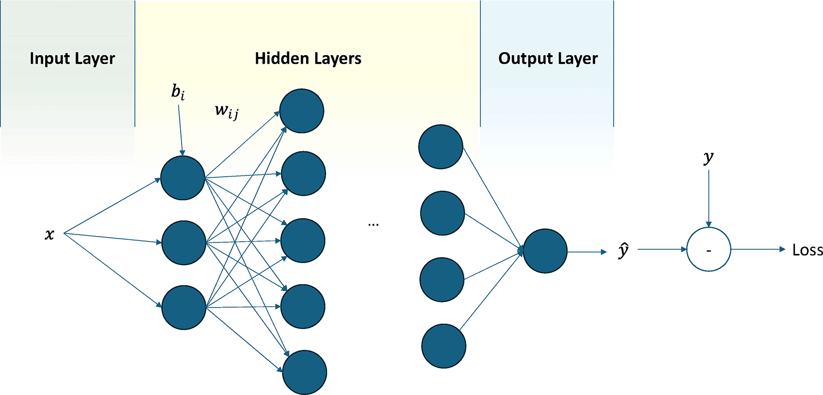
According to the universal approximation theorem, a neural network has the capacity to approximate any function with arbitrary precision¹⁸; however, the required connectivity of the neurons, referred to as network architecture, must be thoroughly examined. Generally, deep architectures, consisting of a multiple hidden layers, are utilized to capture hierarchical features, whereas shallow networks, which consist of fewer layers, are deployed in scenarios where data or computational resources are limited.¹⁹ The training process entails the formulation of a ‘Loss function’ to compare the outputs generated by the neural network $(\hat{y})$ against an established ground truth $(y)$ , followed by the targeted adjustment of weights and biases.

In the context of PINNs, neural networks are extended to incorporate physical constraints directly into the training process. Unlike conventional neural networks that rely solely on data-driven learning, PINNs integrate information from governing equations and boundary conditions into the loss function, ensuring that the learned solutions adhere to underlying physical laws.¹ The loss function in PINNs comprises three main components: (i) a data loss term that ensures consistency with available observations, (ii) a physics loss term that enforces compliance with differential equations, and (iii) a boundary/initial condition loss term that satisfies prescribed constraints.

PINNs can be categorized into two main types: data-driven approaches, which infer hidden relationships from experimental data, and physics-driven approaches, which directly solve differential equations while enforcing physical consistency.^20,21 It has been demonstrated that the integration of physical principles into neural network architectures improves their interpretability, generalizability, and applicability across a diverse array of scientific and engineering challenges.²² This study focuses on the latter category, specifically employing physics-driven PINNs to solve differential equations while addressing challenges associated with unbalanced loss terms.

2.2 Term scaling

An effective introduction to the scaling treatment of differential equations is presented herein, based on generalized scaling methods.²³ The objective of scaling is to render both the dependent and independent variables dimensionless, while simultaneously positioning them within the unit range. Each variable is normalized using a characteristic quantity relevant to the specific problem. For instance, the spatial variable may be normalized in relation to the length of a structure. Subsequently, all terms and derivatives appearing in the differential equation are expressed in terms of their dimensionless equivalents. Any unestablished scaling coefficients are approximated by requiring that the corresponding terms of the equation remain proximate to unity. Upon resolving the equation in its normalized form, a reverse process is employed to retrieve the solution in the physical domain.

The proposed method, referred to as Scaled Equation-Enhanced Physics Informed Neural Network (SEE-PINN), for handling unbalanced loss terms in PINNs, is built directly on this scaling framework. By ensuring that all terms of the differential equation operate on comparable scales before constructing the loss function, our approach simplifies implementation while improving optimization efficiency. This is demonstrated through its application to two distinct mechanical problems: an elastic rod and an Euler beam. In both cases, the exact same procedural steps are followed, emphasizing the method’s consistency and ease of use. The only variation lies in the number of variables and functions requiring normalization, reinforcing its generality and adaptability across different types of differential equations. The following paragraphs provide the numerical formulation of equations typically encountered in the literature, incorporating this systematic scaling approach.

2.2.1 Elastic rod

The response of an elastic rod is described by the 1D Poisson equation:

(2)

\frac{d}{dx} [E (x) \cdot A (x) \cdot \frac{du}{dx}] + p (x) = 0, x \in [0, L]

where

L

is the length,

E

is the Young’s modulus,

A

is the cross-sectional area,

p

is the applied load and

u

corresponds to the pursued axial displacement. The fact that all quantities are presumed to vary arbitrarily with respect to

x

, prevents the derivation of general analytic solutions. Eq. (2) can be expanded as

(3)

E_{x} A u_{x} + E A_{x} u_{x} + EA u_{xx} + p = 0

where subscript

x

indicates differentiation.

To derive the normalized formulation of Eq. (3) each term is normalized using a characteristic quantity. Initially, the normalized spatial variable is defined as

(4)

\bar{x} = \frac{x}{x_{c}} \to x = x_{c} \cdot \bar{x} \to \frac{d \bar{x}}{dx} = \frac{1}{x_{c}}

where

x_{c}

is the scaling coefficient. In the same sense, the Young’s modulus, the cross-sectional area, the axial displacement and the applied load can be expressed in their respective normalized forms:

(5)

\bar{E} \equiv \bar{E} (\bar{x}) = \frac{E (x)}{e_{c}} \to E (x) = e_{c} \cdot \bar{E} (\bar{x})

(6)

\bar{A} \equiv \bar{A} (\bar{x}) = \frac{A (x)}{a_{c}} \to A (x) = a_{c} \cdot \bar{A} (\bar{x})

(7)

\bar{u} \equiv \bar{u} (\bar{x}) = \frac{u (x)}{u_{c}} \to u (x) = u_{c} \cdot \bar{u} (\bar{x})

(8)

\bar{p} \equiv \bar{p} (\bar{x}) = \frac{p (x)}{p_{c}} \to p (x) = p_{c} \cdot \bar{p} (\bar{x})

where

e_{c}, a_{c}, u_{c}, p_{c}

are scaling coefficients to ensure that the range of

\bar{E}, \bar{A}, \bar{u}

and

\bar{p}

is normalized to

[0, 1]

. The following reasonable assumptions are made for Eqs. (4)-(8):

(9)

x_{c} = L, e_{c} = max E (x), a_{c} = max A (x), p_{c} = max | p (x) |

For $u_{c}$ no assumption can be made at this point, since the value of $u (x)$ remains unknown; consequently, it must be approximated through an alternative method.

The respective spatial derivatives appearing in Eq. (3) are expressed in normalized form using Eqs.(4)-(8):

(10)

E_{x} (x) = \frac{dE (x)}{dx} = \frac{d}{dx} [e_{c} \bar{E} (\bar{x})] = e_{c} \frac{d \bar{E} (\bar{x})}{d \bar{x}} \frac{d \bar{x}}{dx} = \frac{e_{c}}{x_{c}} {\bar{E}}_{\bar{x}} (\bar{x})

(11)

A_{x} (x) = \frac{dA (x)}{dx} = \frac{d}{dx} [a_{c} \bar{A} (\bar{x})] = a_{c} \frac{d \bar{A} (\bar{x})}{d \bar{x}} \frac{d \bar{x}}{dx} = \frac{a_{c}}{x_{c}} {\bar{A}}_{\bar{x}} (\bar{x})

(12)

u_{x} (x) = \frac{du (x)}{dx} = \frac{d}{dx} [u_{c} \bar{u} (\bar{x})] = u_{c} \frac{d \bar{u} (\bar{x})}{d \bar{x}} \frac{d \bar{x}}{dx} = \frac{u}{x_{c}} {\bar{u}}_{\bar{x}} (\bar{x})

(13)

u_{xx} (x) = \frac{d u_{x} (x)}{dx} = \frac{d}{dx} [\frac{u_{c}}{x_{c}} {\bar{u}}_{\bar{x}} (\bar{x})] = \frac{u_{c}}{x_{c}} \frac{d {\bar{u}}_{\bar{x}} (\bar{x})}{d \bar{x}} \frac{d \bar{x}}{dx} = \frac{u}{x_{c}^{2}} {\bar{u}}_{\bar{x} \bar{x}} (\bar{x})

Then, Eq. (3) can be reformulated utilizing the normalized quantities:

(14)

\frac{e_{c}}{x_{c}} {\bar{E}}_{\bar{x}} \cdot a_{c} \bar{A} \cdot \frac{u_{c}}{x_{c}} {\bar{u}}_{\bar{x}} + e_{c} \bar{E} \cdot \frac{a_{c}}{x_{c}} {\bar{A}}_{\bar{x}} \cdot \frac{u_{c}}{x_{c}} {\bar{u}}_{\bar{x}} + e_{c} \bar{E} \cdot a_{c} \bar{A} \cdot \frac{u_{c}}{x_{c}^{2}} {\bar{u}}_{\bar{x} \bar{x}} + p_{c} \bar{p} = 0

After simplifying the equation:

(15)

{\bar{E}}_{\bar{x}} \cdot \bar{A} \cdot {\bar{u}}_{\bar{x}} + \bar{E} \cdot {\bar{A}}_{\bar{x}} \cdot {\bar{u}}_{\bar{x}} + \bar{E} \cdot \bar{A} \cdot {\bar{u}}_{\bar{x} \bar{x}} + \frac{p_{c} \cdot x_{c}^{2} \cdot \bar{p}}{e_{c} \cdot a_{c} \cdot u_{c}} = 0

To confine the last term within the interval [0,1] as well, its coefficient is set equal unity, yielding the value of the normalizing parameter $u_{c}$ :

(16)

\frac{p_{c} \cdot x_{c}^{2}}{e_{c} \cdot a_{c} \cdot u_{c}} = 1 \to u_{c} = \frac{p_{c} \cdot x_{c}^{2}}{e_{c} \cdot a_{c}}

2.2.2 Elastic Euler beam

The response of an elastic Euler beam is described by the well-known equation:

(17)

\frac{d^{2}}{d x^{2}} [E (x) \cdot I (x) \cdot \frac{d^{2} w}{d x^{2}}] - p (x) = 0, x \in [0, L]

where

L

is the length,

E

is the Young’s modulus,

I

is moment of inertia,

p

is the applied load and

w

is the pursued transverse deflection. All quantities are presumed to vary with respect to

x

, which precludes general analytic solutions. Eq. (17) can be expanded as

(18)

(E_{xx} I + 2 E_{x} I_{x} + E I_{xx}) \cdot w_{xx} + 2 (E_{x} I + E I_{x}) \cdot w_{xxx} + EI \cdot w_{xxxx} - p = 0

where subscript

x

indicates differentiation.

To derive the normalized formulation of Eq. (18), each term is normalized using a characteristic quantity. The normalized spatial variable, Young modulus and applied load are defined again as in Eqs. (4), (5) and (8) using the same scaling coefficients as in Eq. (9). In the same sense the normalized inertial moment and transverse deflection are defined as:

(19)

\bar{I} \equiv \bar{I} (\bar{x}) = \frac{I (x)}{i_{c}} \to I (x) = i_{c} \cdot \bar{I} (\bar{x})

(20)

\bar{w} \equiv \bar{w} (\bar{x}) = \frac{w (x)}{w_{c}} \to w (x) = w_{c} \cdot \bar{w} (\bar{x})

where

i_{c}, w_{c}

are scaling coefficients to ensure that the range of

\bar{I}

and

\bar{w}

is normalized to

[0, 1]

. A reasonable assumption for

i_{c}

is:

(21)

i_{c} = max I (x)

but, again, no assumption can be made for

w_{c}

, and it needs to be determined.

The respective spatial derivatives appearing in Eq. (18) are expressed in normalized form:

(22)

E_{x} (x) = \frac{dE (x)}{dx} = \frac{d}{dx} [e_{c} \bar{E} (\bar{x})] = e_{c} \frac{d \bar{E} (\bar{x})}{d \bar{x}} \cdot \frac{d \bar{x}}{dx} = \frac{e_{c}}{x_{c}} \cdot {\bar{E}}_{\bar{x}} (\bar{x})

(23)

E_{xx} (x) = \frac{d E_{x} (x)}{dx} = \frac{d}{d \bar{x}} [\frac{e_{c}}{x_{c}} {\bar{E}}_{\bar{x}} (\bar{x})] \cdot \frac{d \bar{x}}{dx} = \frac{e_{c}}{x_{c}^{2}} {\bar{E}}_{\bar{x} \bar{x}} (\bar{x})

(24)

I_{x} (x) = \frac{dI (x)}{dx} = \frac{d}{dx} [i_{c} \bar{I} (\bar{x})] = i_{c} \frac{d \bar{I} (\bar{x})}{d \bar{x}} \cdot \frac{d \bar{x}}{dx} = \frac{i_{c}}{x_{c}} \cdot {\bar{I}}_{\bar{x}} (\bar{x})

(25)

I_{xx} (x) = \frac{d I_{x} (x)}{dx} = \frac{d}{d \bar{x}} [\frac{i_{c}}{x_{c}} {\bar{I}}_{\bar{x}} (\bar{x})] \cdot \frac{d \bar{x}}{dx} = \frac{i_{c}}{x_{c}^{2}} {\bar{I}}_{\bar{x} \bar{x}} (\bar{x})

(26)

w_{x} (x) = \frac{dw (x)}{dx} = \frac{d}{dx} [w_{c} \bar{w} (\bar{x})] = w_{c} \frac{d \bar{w} (\bar{x})}{d \bar{x}} \cdot \frac{d \bar{x}}{dx} = \frac{w_{c}}{x_{c}} \cdot {\bar{w}}_{\bar{x}} (\bar{x})

(27)

w_{xx} (x) = \frac{d w_{x} (x)}{dx} = \frac{d}{d \bar{x}} [\frac{w_{c}}{x_{c}} {\bar{w}}_{\bar{x}} (\bar{x})] \cdot \frac{d \bar{x}}{dx} = \frac{w_{c}}{x_{c}^{2}} {\bar{w}}_{\bar{x} \bar{x}} (\bar{x})

(28)

w_{xxx} (x) = \frac{d w_{xx} (x)}{dx} = \frac{d}{d \bar{x}} [\frac{w_{c}}{x_{c}^{2}} {\bar{w}}_{\bar{x} \bar{x}} (\bar{x})] \cdot \frac{d \bar{x}}{dx} = \frac{w_{c}}{x_{c}^{3}} {\bar{w}}_{\bar{x} \bar{x} \bar{x}} (\bar{x})

(29)

w_{xxxx} (x) = \frac{d w_{xxx} (x)}{dx} = \frac{d}{d \bar{x}} [\frac{w_{c}}{x_{c}^{3}} {\bar{w}}_{\bar{x} \bar{x} \bar{x}} (\bar{x})] \cdot \frac{d \bar{x}}{dx} = \frac{w_{c}}{x_{c}^{4}} {\bar{w}}_{\bar{x} \bar{x} \bar{x} \bar{x}} (\bar{x})

Then, Eq. (18) can then be recast using the normalized quantities:

(30)

\bar{E} \bar{I} {\bar{w}}_{\bar{x} \bar{x} \bar{x} \bar{x}} + 2 ({\bar{E}}_{\bar{x}} \bar{I} + \bar{E} {\bar{I}}_{\bar{x}}) {\bar{w}}_{\bar{x} \bar{x} \bar{x}} + ({\bar{E}}_{\bar{x} \bar{x}} \bar{I} + 2 {\bar{E}}_{\bar{x}} {\bar{I}}_{\bar{x}} + \bar{E} {\bar{I}}_{\bar{x} \bar{x}}) {\bar{w}}_{\bar{x} \bar{x}} - \frac{p_{c} \cdot x_{c}^{4}}{e_{c} \cdot i_{c} \cdot w_{c}} \bar{p} = 0

In order to constrain the last term in [0,1] as well, its coefficient is set equal unity, yielding the value of the normalizing parameter $w_{c}$ :

(31)

\frac{p_{c} \cdot x_{c}^{4}}{e_{c} \cdot i_{c} \cdot w_{c}} = 1 \to w_{c} = \frac{p_{c} \cdot x_{c}^{4}}{e_{c} \cdot i_{c}}

3. Technical aspects and performance assessment

In this section, the architecture of the proposed SEE-PINN framework is first introduced, detailing the network structure, activation functions, training procedure, and implementation of the term-scaling approach. This ensures a comprehensive understanding of the methodology before proceeding to validation and performance evaluation.

Following this, the proposed method is validated through a series of test cases and subsequently compared to solutions found in the literature to illustrate its computational efficiency. The objective is not to undermine existing methods but to demonstrate that they can benefit from our approach and achieve enhanced accuracy and robustness.

Both simple and complex case studies are examined concerning the problems associated with the elastic rod and the elastic Euler beam to validate the proposed method. For straightforward cases, the solution obtained through PINNs is compared against analytical solutions. In more complex scenarios, where no analytical solution is available, the PINN solution is contrasted with numerical solutions.

3.1 Network architecture

Following the term scaling methodology description, a comprehensive architecture is provided here. The fundamental framework is presented for the rod and beam problems. This design is intended to be easily adaptable, enabling other researchers to extend it to various problems with minimal effort.

The proposed approach begins with a normalization step applied to the coefficients of the ODE terms before they are introduced into the input layer. These normalized coefficients, together with the neural network outputs, undergo automatic differentiation to compute the gradients of the required to form the ODE. The resulting terms are then incorporated into the loss function, which typically consists of one term for the ODE residual and additional terms for each boundary condition. In this work, the mean squared error is employed for the terms of the loss function. If the total loss converges below a predefined threshold, the process proceeds to de-normalization, producing the final solution. Otherwise, backpropagation updates the network’s weights and biases until convergence is reached.

The architecture for the elastic rod is illustrated in Figure 2 and can be readily adapted to the beam problem (or other related problems) by modifying the predicted quantities and the computed gradients. Specifically, for the beam, the output variable changes from the axial displacement $u$ (for the rod) to the transverse deflection $w$ , while the required gradients expand significantly. The rod problem involves computing $E_{x}, A_{x}, u_{x}$ and $u_{xx}$ , whereas the beam problem requires additional terms, namely $E_{xx}, I_{x}, I_{xx}, w_{x}, w_{xx}, w_{xxx}$ and $w_{xxxx}$ . Likewise, the rod problem is solved using two boundary conditions, e.g. a Dirichlet and a Neumann condition (denoted in Figure 2 by $L_{D}$ and $L_{N}$ respectively), while the beam problem requires four boundary conditions. Although the mathematical complexity increases significantly (as detailed in the respective sections), the transition from the rod to the beam remains conceptually straightforward. The same principle applies when extending the approach to other problems.

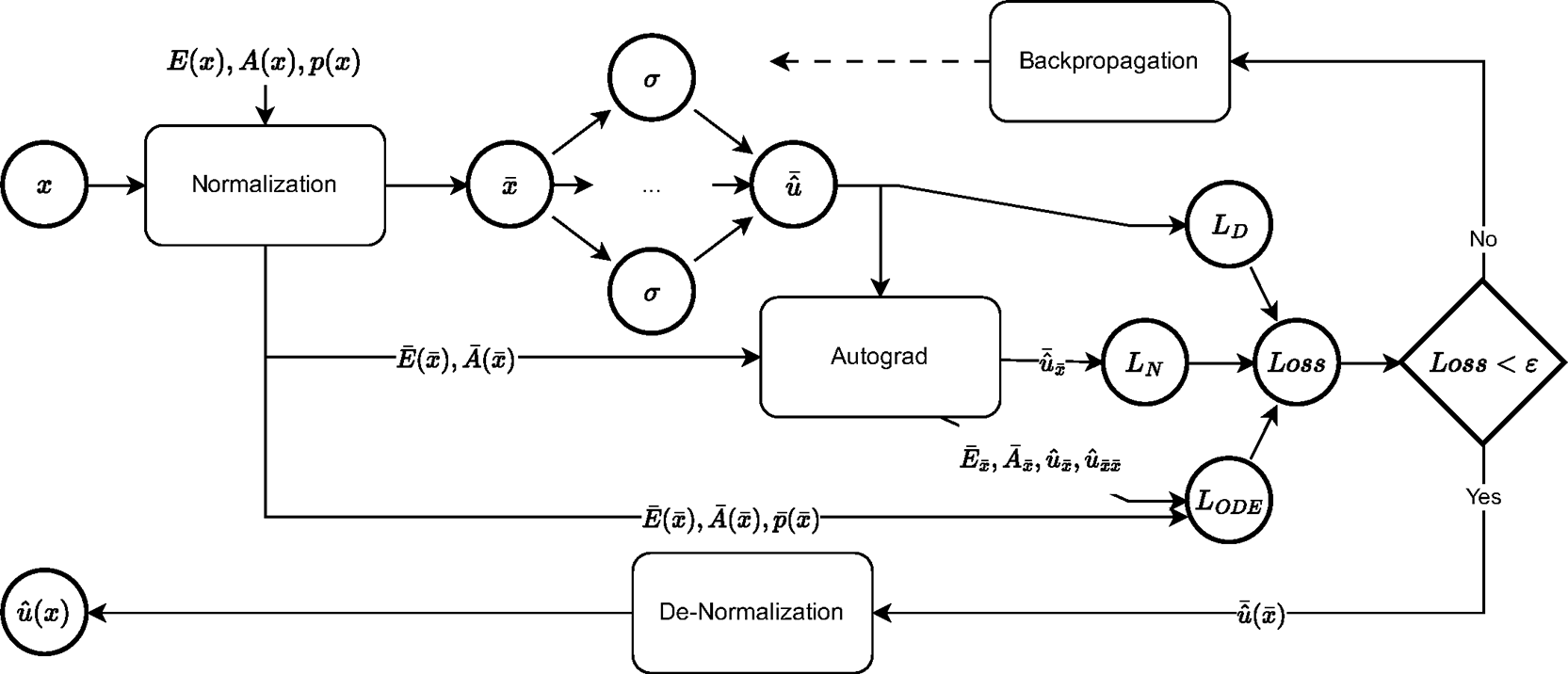
Figure 2. Network architecture for the problem of the elastic rod.

The network is implemented in PyTorch, to take advantage of computational optimizations, and automatic computing (Autograd) of derivatives in the loss function.

3.2 Validations

3.2.1 Fixed uniform rod with distributed load

Statement of the problem. This represents a straightforward scenario. A homogenous rod with a uniform cross-section is subjected to an axially distributed load. The left end of the rod is fixed, while the right one is free. The axial displacement along the rod is analyzed. Numerical values are:

(32)

E = 200 GPa, A = 1 c m^{2}, p (x) = 1000 x^{2} \frac{N}{m}, L = 1 m

Since properties are constant along the rod, Eq. (2) is diminished to

(33)

EA \frac{d^{2} u}{d x^{2}} + p (x) = 0

with boundary conditions

(34)

\begin{matrix} Displacement at x = 0 : & u (0) = 0 \\ Force at x = L : & EA u_{x} (L) = 0 \end{matrix}

The analytic solution is

(35)

u (x) = - \frac{x^{4}}{240000} + \frac{x}{60000}

SEE-PINN solution. An appropriate neural network is designed to approximate the displacement field of the rod. The input of the neural network is the spatial coordinate $x$ , and its output is the predicted displacement $\hat{u} (x)$ . The network consists of only one fully connected layer, with 10 neurons, and each neuron employs the tanh activation function. The network is trained at 75 points using the Adam optimizer with learning rate 0.01 for 5000 epochs.

Comparison and error analysis. The predicted solution the PINN is validated against the analytical solution – Eq. (35). Figure 3a demonstrates that the analytic and the PINN solution are indistinguishable from each other, as verified by the parity plot in Figure 3b. The prediction quality is further assessed using the normalized relative error, where the relative error is scaled according to the magnitude of the displacement values to prevent numerical artifacts from division by very small numbers.

(36)

e (x) = \frac{| u (x) - \hat{u} (x) |}{| u (x) + O (u) |} \cdot 100 %

Figure 3. SEE-PINN vs. Analytic solution for case 3.2.1.

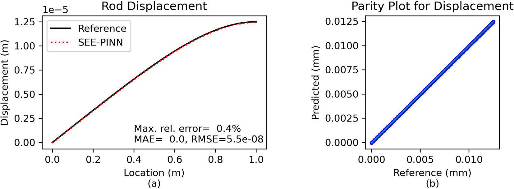
(a) Direct comparison of predictions. (b) Parity plot of predicted vs. reference solution.

The maximum relative error is ca. 0.4%, which demonstrates the PINN approach achieves nearly exact agreement with the analytical solution.

3.2.2 Fixed rod with variable cross-section and distributed load

Statement of the problem. This case builds upon the previous problem by introducing a nonlinear variation in the cross-sectional area.

(37)

A (x) = [2 + sin (2 π \frac{x}{L})] c m^{2}

while keeping all other parameters unchanged, increasing the complexity of the analysis.

SEE-PINN solution. The same neural network has been employed to approximate the displacement field of the rod; i.e. one fully connected layer, with 10 neurons, and each neuron employs the tanh activation function. The network is trained at 75 points using the Adam optimizer with learning rate 0.01 for 5000 epochs.

Comparison and error analysis. The predicted solution is compared against a numerical reference for validation. Figure 4 illustrates that the analytic and the PINN solution are again indistinguishable. With a maximum relative error of approximately 0.04%, the PINN approach demonstrates an excellent agreement with the analytical solution.

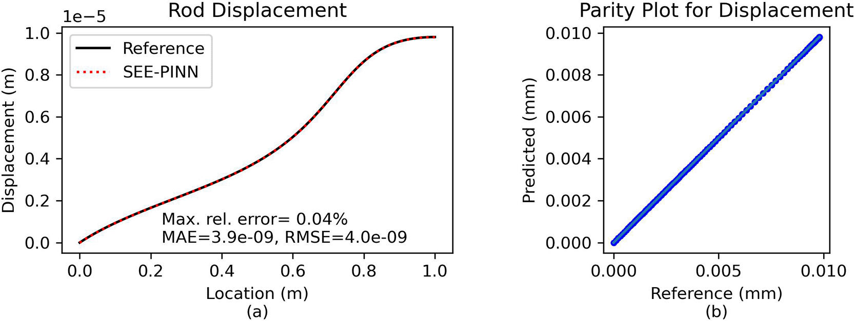
Figure 4. SEE-PINN vs. Analytic solution for case 3.2.2.

(a) Direct comparison of predictions. (b) Parity plot of predicted vs. reference solution.

3.2.3 Fixed rod with variable Young’s modulus and cross-section, and distributed load

Statement of the problem. The complexity is further increased by incorporating a nonlinear variation in the Young’s modulus of the rod.

(38)

E (x) = 200 \cdot (1 - tanh x) GPa

while preserving the other parameters; the cross-sectional area still varies according to Eq. (37). This variation is designed to mimic the behavior of exotic materials, similar to those found in advanced metamaterials, or the properties of damaged materials.

SEE-PINN solution. The same neural network has been employed to approximate the displacement field of the rod; i.e. one fully connected layer, with 10 neurons, and each neuron employs the tanh activation function. The network is trained at 75 points using the Adam optimizer with learning rate 0.01 for 5000 epochs.

Comparison and error analysis. The predicted solution validated against is validated against a numerical reference. As shown in Figure 5, the analytical and PINN solutions are virtually identical. The maximum relative error is approximately 0.05%, indicating that the PINN approach achieves an almost exact match with the analytical solution.

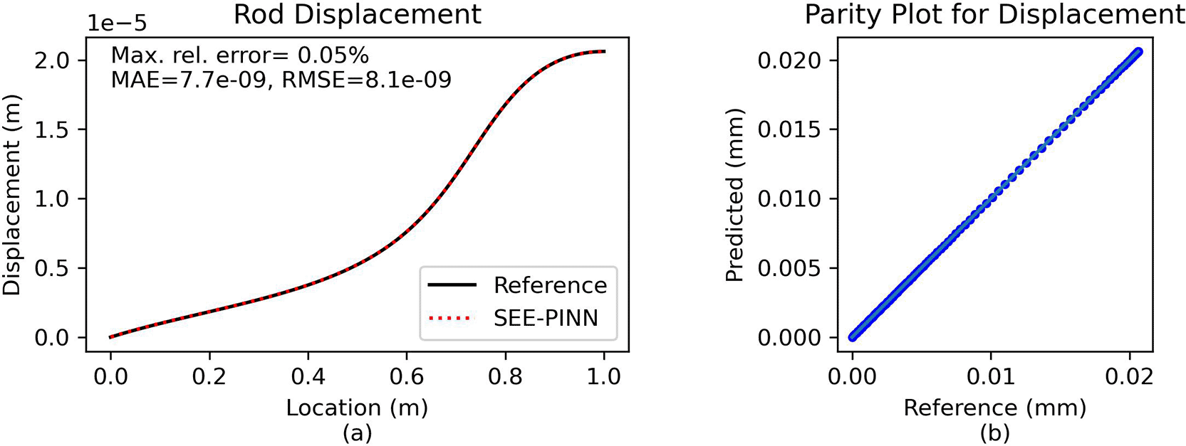
Figure 5. SEE-PINN vs. Analytic solution for case 3.2.3.

(a) Direct comparison of predictions. (b) Parity plot of predicted vs. reference solution.

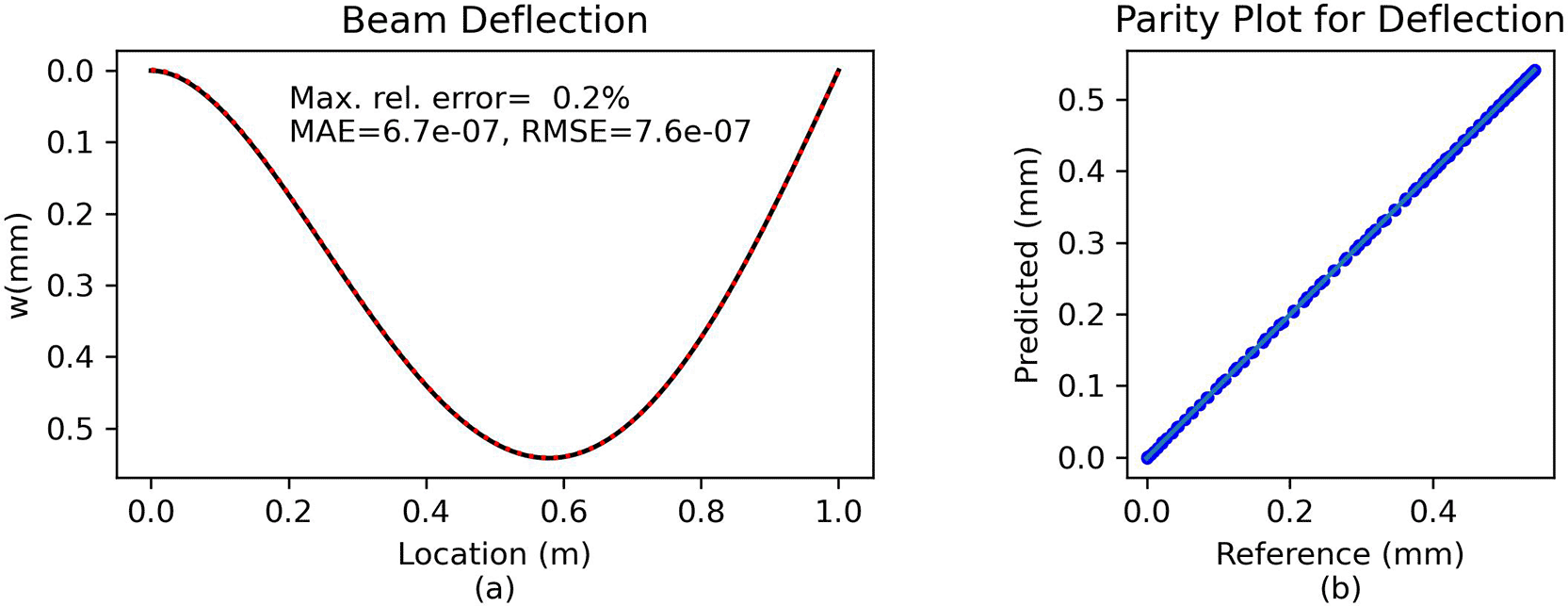
3.2.4 Uniform Euler beam with distributed load

Statement of the problem. The second part of the validation examines three beam problems. The first case considers a uniform, homogeneous elastic beam with a length of $L = 1$ m. The beam has a rectangular cross-section of $b = 6 cm, h = 1 cm$ and is composed of a material with $E = 200 GPa$ . The left end of the rod is fixed, while the right one is simply supported. The beam is subjected to a transverse load of $p (x) = 100 N / m$ , and its transverse deflection is analyzed.

This problem can be easily solved through the analytical solution of Eq. (17) with constant properties and boundary conditions:

(39)

\begin{matrix} Deflection at x = 0 : & w (0) = 0 \\ Rotation at x = 0 : & w^{'} (0) = 0 \\ Deflection at x = L : & w (L) = 0 \\ Moment at x = L : & EI w^{''} (L) = 0 \end{matrix}

The analytic solution is:

(40)

w (x) = \frac{x^{4}}{240} - \frac{x^{3}}{96} + \frac{x^{2}}{160}

SEE-PINN solution. An appropriate neural network is designed to approximate the deflection of the beam. The input of the neural network is the spatial coordinate $x$ , and its output is the predicted transverse displacement $\hat{w} (x)$ . The network consists of only one fully connected layer, with 10 neurons, and each neuron employs the tanh activation function. The network is trained at 75 points using the Adam optimizer with learning rate 0.001 for 10000 epochs.

Comparison and error analysis. The predicted solution is validated against the analytical reference ( Figure 6), showing that the analytical and PINN solutions are virtually identical ( Figure 6a); this is further supported by the parity plot ( Figure 6b), where all data points practically lay along the diagonal. With a maximum relative error of approximately 0.2%, the PINN approach achieves exceptional accuracy in comparison to the analytical solution.

Figure 6. SEE-PINN vs. Analytic solution for case 3.2.4.

(a) Direct comparison of predictions. (b) Parity plot of predicted vs. reference solution.

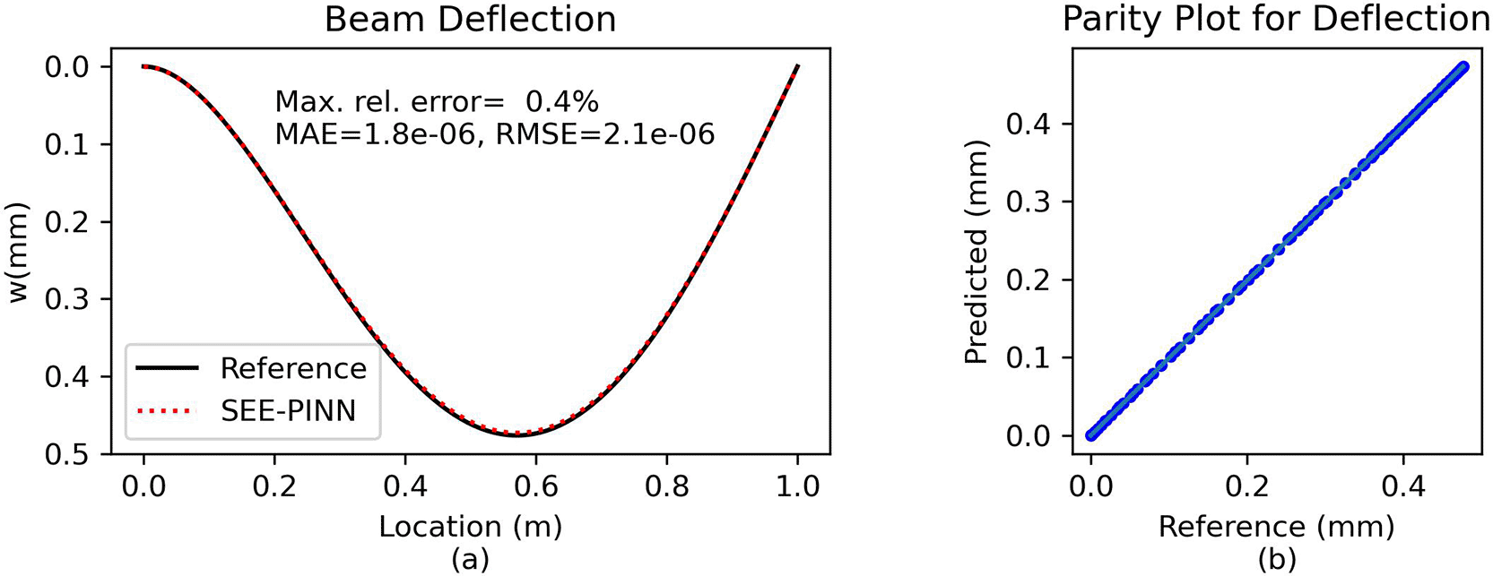
3.2.5 Euler beam with variable cross-section and distributed load

Statement of the problem. This case builds upon the previous problem by introducing a nonlinear transition in the inertial moment of the cross-section, represented by $I$ :

(41)

I (x) = I_{0} \cdot [1 + 0.5 x - 0.25 x^{2}], I_{0} = \frac{b \cdot h^{3}}{12}

while keeping all other parameters unchanged, increasing the complexity of the analysis.

PINN solution. A shallow architecture has been employed to approximate the deflection of the beam; i.e. one fully connected layer, with 10 neurons, and each neuron employs the tanh activation function. The network is trained at 75 points using the Adam optimizer with learning rate 0.001 for 10000 epochs.

Comparison and error analysis. The predicted solution is compared against a numerical reference for validation. Figure 7 illustrates that the analytic and the PINN solution are again indistinguishable. With a maximum relative error of approximately 0.35%, the PINN approach demonstrates an excellent agreement with the analytical solution.

Figure 7. SEE-PINN vs. Numerical solution for case 3.2.5.

(a) Direct comparison of predictions. (b) Parity plot of predicted vs. reference solution.

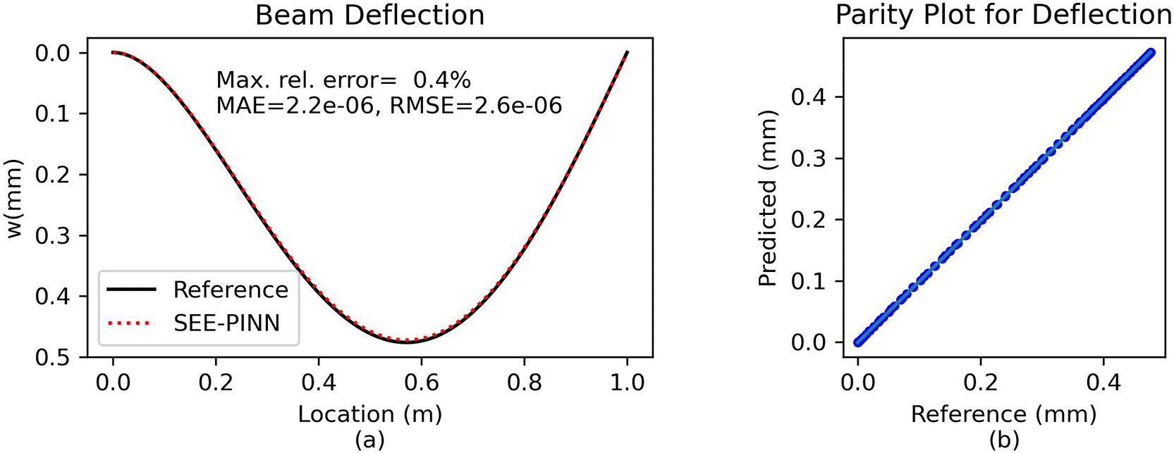
3.2.6 Euler beam with variable Young’s modulus and cross-section, and distributed load

Statement of the problem. The complexity is further enhanced by introducing a nonlinear variation in the Young’s modulus of the beam,

(42)

E (x) = 200 \cdot (1 - 0.25 x - 0.5 x^{2}) GPa

while keeping all other parameters unchanged. The cross-sectional area continues to vary according to Eq. (41).

SEE-PINN solution. The same neural network has been employed to approximate the deflection of the beam; one fully connected layer, with 10 neurons, and each neuron employs the tanh activation function. The network is trained at 75 points using the Adam optimizer with learning rate 0.001 for 10000 epochs.

Comparison and error analysis. The predicted solution is compared against a numerical reference for validation. Figure 8 illustrates that the analytic and the PINN solution are again indistinguishable. With a maximum relative error of approximately 0.4%, the PINN approach demonstrates an excellent agreement with the analytical solution.

Figure 8. SEE-PINN vs. Numerical solution for case 3.2.6.

(a) Direct comparison of predictions. (b) Parity plot of predicted vs. reference solution.

3.3 Performance

The performance of the introduced methodology is assessed by comparison to existing models. The objective is to demonstrate that the suggested approach yields the same solution while utilizing significantly fewer computational resources. Given that the precise technical details of each study are not known, theoretical estimates of computational requirements and complexity have been derived from the respective network architectures.

3.3.1 Performance metric

This analysis evaluates the floating point operations (FLOPs) required for both the forward and backward passes as a key metric for assessing the performance of a neural network. While other metrics, such as the memory needed to store weights, biases, and intermediate results, could also be considered, a more detailed examination of these factors is beyond the scope of this paper.

According to Eq. (1), a neuron in fully connected layer performs three basic operations: (a) multiplication of every input with a weight, i.e. $N_{in}$ operations, (b) summation of all input-weight products, i.e. $N_{in} - 1$ operations, and (c) addition of a bias, i.e. $1$ operation. Thus, for a layer with $N_{in}$ inputs an $N_{out}$ outputs, the required number of FLOPs for a forward pass is:

(43)

F_{FWD}^{L} (N_{in}, N_{out}) = [N_{in} + (N_{in} - 1) + 1] \cdot N_{out} = 2 N_{in} N_{out}

The backpropagation process is more complex than the forward pass and is assumed to require three times as many FLOPs; $F_{BKD} = 3 F_{FWD}$ . For simplicity, the computations needed for activation functions are considered minimal, so any additional overhead calculations—which may vary by implementation—are not included. Therefore, the total computational load is calculated by multiplying the total number of FLOPs required for both the forward pass and backpropagation by the number of training points and the number of epochs.

3.3.2 Case studies

Case 1.

Wang et al.²⁴ have conducted simulations on a 10 m long homogeneous rod featuring a cross-sectional area of 1 m², composed of a material characterized by a Young’s modulus of 175 Pa. The rod was fixed at both ends and subjected to a distributed load:

(44)

b (x) = - \frac{4 π^{2} {(x - 2.5)}^{2} - 2 π}{e^{π {(x - 2.5)}^{2}}} - \frac{8 π^{2} {(x - 7.5)}^{2} - 4 π}{e^{π {(x - 7.5)}^{2}}}

The authors addressed the problem by utilizing a PINN comprising 6 hidden layers, with each layer containing 512 neurons employing the ReLU activation function. The model was trained for $N_{e} = 50,000$ epochs using $N_{p} = 100$ data points.

The computational cost for a forward pass is the total sum of FLOPs for the input layer, the six hidden layers, and the output layer, i.e.

(45)

\begin{matrix} F_{FWD} & = F_{FWD}^{L} (1, 512) + 6 F_{FWD}^{L} (512, 512) + F_{FWD}^{L} (512, 1) \\ = [2 \cdot 1 \cdot 512] + 6 \cdot [2 \cdot 512 \cdot 512] + [2 \cdot 512 \cdot 1] \\ = 3 147 776 FLOPs \end{matrix}

When including the cost of back-propagation and considering the number of training points, the total computational cost becomes:

(46)

F_{tot} = (F_{FWD} + F_{BKD}) \cdot N_{p} \cdot N_{e} = 4 F_{FWD} \cdot N_{p} \cdot N_{e} \approx 63 TFLOPs

The solution was subsequently validated against an analytical benchmark solution:

(47)

u (x) = \frac{1}{EA} \cdot (e^{- π {(x - 2.5)}^{2} - e^{- 6.25 π}}) + \frac{2}{EA} (e^{- π {(x - 7.5)}^{2}} - e^{- 6.25 π})

The same problem was solved using the proposed approach but with a significantly smaller network, specifically two layers containing 20 neurons each, trained on 100 points for 30,000 epochs. A comparison of the predictions with the provided analytical solution in Figure 9 shows excellent agreement.

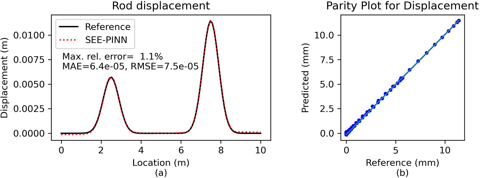
Figure 9. SEE-PINN vs. Analytical solution for case study 1.

(a) Direct comparison of predictions. (b) Parity plot of predicted vs. reference solution.

The computational cost for a forward pass in this configuration is given:

(48)

\begin{matrix} F_{FWD} & = F_{FWD}^{L} (1, 20) + 2 F_{FWD}^{L} (20, 20) + F_{FWD}^{L} (20, 1) \\ = [2 \cdot 1 \cdot 20] + 2 \cdot [2 \cdot 20 \cdot 20] + [2 \cdot 20 \cdot 1] \\ = 1600 FLOPs \end{matrix}

and the total cost is

F_{tot} = 20.16 GFLOPs

which is three orders of magnitude lower than the original approach.

Case 2.

Singh et al.²⁵ simulated the bending of a 1 m long homogeneous Euler beam with a moment of inertia I = 1.0, made of a material with Young’s modulus of 1.0 Pa. The beam was fixed at one end and subjected to a distributed load:

(49)

p (x) = 1 - x

To solve this problem, the authors employed a PINN with 5 hidden layers, each containing 50 neurons using the tanh activation function. The model was trained for $N_{e} = 300$ epochs using $N_{p} = 51$ data points.

The computational cost for a forward pass is the total sum of FLOPs for the input layer, the five hidden layers, and the output layer, i.e.

(50)

\begin{matrix} F_{FWD} & = F_{FWD}^{L} (1, 50) + 5 F_{FWD}^{L} (50, 50) + F_{FWD}^{L} (50, 1) \\ = [2 \cdot 1 \cdot 50] + 5 \cdot [2 \cdot 50 \cdot 50] + [2 \cdot 50 \cdot 1] \\ = 25 200 FLOPs \end{matrix}

Taking into account the cost of back-propagation, the number of training points and the number of epochs, the total computational cost is given by:

(51)

F_{tot} = (F_{FWD} + F_{BKD}) \cdot N_{p} \cdot N_{e} = 4 F_{FWD} \cdot N_{p} \cdot N_{e} \approx 1.54 GFLOPs

The solution was validated against an analytical benchmark solution:

(52)

w (x) = - \frac{x^{5}}{120} + \frac{x^{4}}{24}

The same problem was solved using the proposed approach but with a significantly smaller network: a single hidden layer with 10 neurons, trained on 75 points for 1,000 epochs. As shown in Figure 10, the predictions closely match the analytical solution, demonstrating excellent agreement.

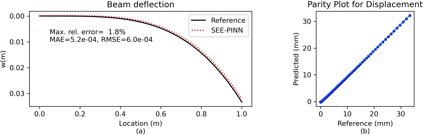
Figure 10. SEE-PINN vs. Analytical solution for case study 2.

(a) Direct comparison of predictions. (b) Parity plot of predicted vs. reference solution.

The computational cost for a forward pass using the SEE-PINN configuration is given:

(53)

\begin{matrix} F_{FWD} & = F_{FWD}^{L} (1, 10) + 1 F_{FWD}^{L} (10, 10) + F_{FWD}^{L} (10, 1) \\ = [2 \cdot 1 \cdot 10] + 5 \cdot [2 \cdot 10 \cdot 10] + [2 \cdot 10 \cdot 1] \\ = 240 FLOPs \end{matrix}

and the total cost is

F_{tot} = 72 MFLOPs

which is two orders of magnitude lower than the original approach. Performance efficiency is visually demonstrated by comparison in Figure 11.

Figure 11. Performance comparisons between SEE-PINN and SOA models in literature (Lower is better).

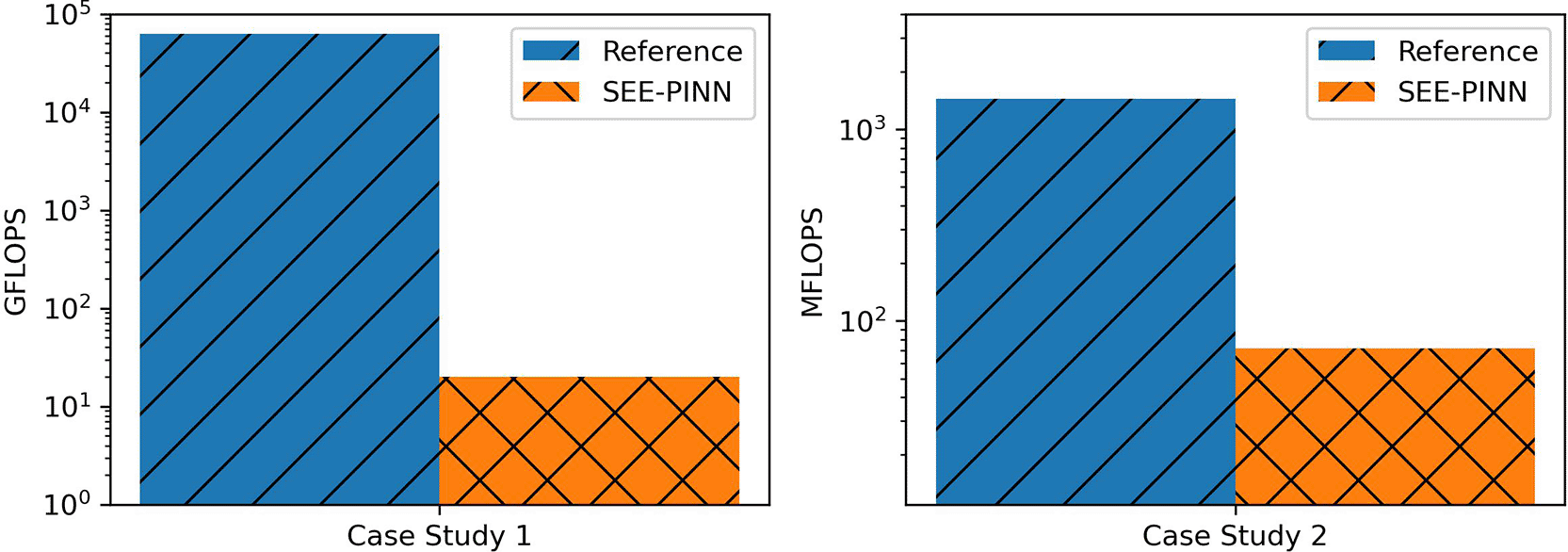
The proposed approach requires 2-3 times less FLOPs.

4. Summary and discussion

The proposed methodology offers an efficient and streamlined approach for solving ordinary differential equations (ODEs) with Physics-Informed Neural Networks (PINNs) by directly scaling the terms of the governing equations, rather than introducing balancing weights within the loss function. Each term is normalized using characteristic physical dimensions, bringing all contributions to a similar order of magnitude close to unity. This ensures numerical consistency and eliminates the need for complex and computationally intensive loss-balancing procedures. The scaled equations are solved within a PINN framework, after which a reverse scaling step restores the solution to the physical domain.

The method has been demonstrated through nonlinear one-dimensional elasticity problems, including rod and Euler–Bernoulli beam cases. The results show that high accuracy can be achieved with extremely compact network architectures – even a single hidden layer with ten nodes – while maintaining negligible maximum percentage error across collocation points. Benchmarking against existing PINN approaches reveals that the proposed scaling strategy reduces floating-point operations (FLOPs) by at least two orders of magnitude, underscoring its potential to deliver substantial computational savings without compromising precision.

While promising, the method also presents opportunities for further development:

1. Optimal Hyperparameter Selection: Automated, self-tuning strategies remain an open research goal to avoid case-by-case manual tuning.
2. Extension to Higher Dimensions: Applying the methodology to 2D and 3D problems, where term coupling increases complexity, is a priority.
3. Highly Nonlinear and Discontinuous Cases: Future work will target problems with sharp gradients, contact conditions, discontinuities, and dynamic effects.
4. Time-Dependent Problems: These can be addressed by treating time as an additional dimension or by adopting time-aware neural architectures such as LSTMs.

In conclusion, the proposed scaling-based PINN framework (SEE-PINN) demonstrates that direct differential equation term scaling can fundamentally simplify and accelerate the training of PINNs for nonlinear problems. By completely removing the reliance on elaborate and costly loss-balancing mechanisms, it enables the use of compact, fast, and accurate models that are easier to deploy in real-world engineering settings. The combination of high accuracy, drastic computational savings, and straightforward implementation positions SEE-PINN as a practical and scalable tool, with the potential to reshape how machine learning is applied to challenging differential equation problems in computational mechanics and beyond.

Ethics and consent

Ethical approval and consent were not required.

Data availability

The data required to reproduce graphs and figures are available under CC-BY 4.0 license https://zenodo.org/records/16909058, 10.5281/zenodo.16909058.²⁶

Acknowledgement

The publication of the article in Open Access mode was financially supported by HEAL-Link (HEAL1000 Gateway). The authors employed ChatGPT 4 for proofreading specific paragraphs of this manuscript; however, all ideas, analyses, methods, results and conclusions presented remain solely those of the authors.

References

1. Raissi M, Perdikaris P, Karniadakis GE: Physics-informed neural networks: A deep learning framework for solving forward and inverse problems involving nonlinear partial differential equations. J Comput Phys. 2019; 378: 686–707. Publisher Full Text
2. Wang Y, Yao Y, Guo J, et al.: A practical PINN framework for multi-scale problems with multi-magnitude loss terms. J Comput Phys. 2024; 510: 113112. Publisher Full Text
3. Deguchi S, Asai M: Dynamic & norm-based weights to normalize imbalance in back-propagated gradients of physics-informed neural networks. J Phys Commun. 2023; 7: 075005. Publisher Full Text
4. Xiang Z, Peng W, Liu X, et al.: Self-adaptive loss balanced Physics-informed neural networks. Neurocomputing. 2022; 496: 11–34. Publisher Full Text
5. Li S, Feng X: Dynamic Weight Strategy of Physics-Informed Neural Networks for the 2D Navier–Stokes Equations. Entropy. 2022; 24: 1254. PubMed Abstract | Publisher Full Text | Free Full Text
6. Cao F, Guo X, Dong X, et al.: wbPINN: Weight balanced physics-informed neural networks for multi-objective learning. Applied Soft Computing. 2025; 170: 112632. Publisher Full Text
7. Vemuri SK, Denzler J: Gradient Statistics-Based Multi-Objective Optimization in Physics-Informed Neural Networks. Sensors. 2023; 23: 8665. PubMed Abstract | Publisher Full Text | Free Full Text
8. Wang J, Xiao X, Feng X, et al.: An improved physics-informed neural network with adaptive weighting and mixed differentiation for solving the incompressible Navier–Stokes equations. Nonlinear Dynam. 2024; 112: 16113–16134. Publisher Full Text
9. Wang S, Teng Y, Perdikaris P: Understanding and Mitigating Gradient Flow Pathologies in Physics-Informed Neural Networks. SIAM J Sci Comput. 2021; 43: A3055–A3081. Publisher Full Text
10. Hu Z, Shukla K, Karniadakis GE, et al.: Tackling the curse of dimensionality with physics-informed neural networks. Neural Networks. 2024; 176: 106369. PubMed Abstract | Publisher Full Text
11. Yu J, Lu L, Meng X, et al.: Gradient-enhanced physics-informed neural networks for forward and inverse PDE problems. Comput Methods Appl Mech Engrg. 2022; 393: 114823. Publisher Full Text
12. Han J, Cai Z, Wu Z, et al.: Residual-Quantile Adjustment for Adaptive Training of Physics-informed Neural Network. 2022 IEEE International Conference on Big Data (Big Data). Osaka, Japan: IEEE; 2022; pp. 921–930. Publisher Full Text
13. Son H, Cho SW, Hwang HJ: Enhanced physics-informed neural networks with Augmented Lagrangian relaxation method (AL-PINNs). Neurocomputing. 2023; 548: 126424. Publisher Full Text
14. Luong KA, Le-Duc T, Lee S, et al.: A novel normalized reduced-order physics-informed neural network for solving inverse problems. Engineering with Computers. 2024; 40: 3253–3272. Publisher Full Text
15. Jha N, Mallik E: GPINN with Neural Tangent Kernel Technique for Nonlinear Two Point Boundary Value Problems. Neural Process Lett. 2024; 56: 192. Publisher Full Text
16. Schmidhuber J: Deep learning in neural networks: An overview. Neural Networks. 2015; 61: 85–117. Publisher Full Text
17. LeCun Y, Bengio Y, Hinton G: Deep learning. Nature. 2015; 521: 436–444. Publisher Full Text
18. Cybenko G: Approximation by superpositions of a sigmoidal function. Math Control Signals Systems. 1989; 2: 303–314. Publisher Full Text
19. Zhang C, Bengio S, Hardt M, et al.: Understanding deep learning (still) requires rethinking generalization. Commun ACM. 2021; 64: 107–115. Publisher Full Text
20. Karniadakis GE, Kevrekidis IG, Lu L, et al.: Physics-informed machine learning. Nat Rev Phys. 2021; 3: 422–440. Publisher Full Text
21. Kafkas P, Giannakopoulos G, Rekatsinas C: Solving Linear Elasticity Problems using Physics-Informed Neural Networks. Proceedings of the 13th Hellenic Conference on Artificial Intelligence. Piraeus Greece: ACM; 2024; pp. 1–8. Publisher Full Text
22. Mishra S, Molinaro R: Estimates on the generalization error of physics-informed neural networks for approximating PDEs. IMA J Numer Anal. 2023; 43: 1–43. Publisher Full Text
23. Langtangen HP, Pedersen GK: Scaling of Differential Equations. Cham: Springer International Publishing; 2016. Publisher Full Text
24. Wang J, Mo YL, Izzuddin B, et al.: Exact Dirichlet boundary Physics-informed Neural Network EPINN for solid mechanics. Comput Methods Appl Mech Engrg. 2023; 414: 116184. Publisher Full Text
25. Singh V, Harursampath D, Dhawan S, et al.: Physics-Informed Neural Network for Solving a One-Dimensional Solid Mechanics Problem. Modelling. 2024; 5: 1532–1549. Publisher Full Text
26. Theodosiou T, Rekatsinas C: Dataset for Physics-Informed Neural Networks without Loss Balancing: A Direct Term Scaling Approach for Nonlinear 1D Problems.2025. Publisher Full Text

Comments on this article Comments (0)

Version 1

VERSION 1 PUBLISHED 14 Nov 2025

Author details Author details

¹ Dept. of Energy Systems, University of Thessaly - Larissa, Larissa, Thessalia - Larissa, 41500, Greece
² Institute of Informatics and Telecommunications, Ethniko Kentro Ereunas Physikon Epistemon Demokritos, Athens, Attica, 15341, Greece

Theodosios Theodosiou
Roles: Conceptualization, Formal Analysis, Investigation, Methodology, Software, Supervision, Validation, Visualization, Writing – Original Draft Preparation, Writing – Review & Editing

Christoforos Rekatsinas
Roles: Conceptualization, Formal Analysis, Investigation, Methodology, Validation, Writing – Original Draft Preparation, Writing – Review & Editing

Competing interests

No competing interests were disclosed.

Grant information

The author(s) declared that no grants were involved in supporting this work.

Article Versions (1)

version 1

Published: 14 Nov 2025, 14:1252

https://doi.org/10.12688/f1000research.169129.1

Copyright

© 2025 Theodosiou T and Rekatsinas C. This is an open access article distributed under the terms of the Creative Commons Attribution License, which permits unrestricted use, distribution, and reproduction in any medium, provided the original work is properly cited.

Download

Export To

metrics

	Views	Downloads
F1000Research	-	-
PubMed Central Data from PMC are received and updated monthly.	-	-

Citations

0

SEE MORE DETAILS

CITE

how to cite this article

Theodosiou T and Rekatsinas C. Physics-Informed Neural Networks without Loss Balancing: A Direct Term Scaling Approach for Nonlinear 1D Problems [version 1; peer review: awaiting peer review]. F1000Research 2025, 14:1252 (https://doi.org/10.12688/f1000research.169129.1)

NOTE: If applicable, it is important to ensure the information in square brackets after the title is included in all citations of this article.

track

receive updates on this article

Track an article to receive email alerts on any updates to this article.

Open Peer Review

Comments on this article Comments (0)

Version 1

VERSION 1 PUBLISHED 14 Nov 2025

Open Peer Review

Reviewer Status

AWAITING PEER REVIEW

Comments on this article

All Comments(0)

Add a comment

Sign up for content alerts

Browse by related subjects

[1] 1. Raissi M, Perdikaris P, Karniadakis GE: Physics-informed neural networks: A deep learning framework for solving forward and inverse problems involving nonlinear partial differential equations. J Comput Phys. 2019; 378: 686–707. Publisher Full Text

[2] 2. Wang Y, Yao Y, Guo J, et al.: A practical PINN framework for multi-scale problems with multi-magnitude loss terms. J Comput Phys. 2024; 510: 113112. Publisher Full Text

[3] 3. Deguchi S, Asai M: Dynamic & norm-based weights to normalize imbalance in back-propagated gradients of physics-informed neural networks. J Phys Commun. 2023; 7: 075005. Publisher Full Text

[4] 4. Xiang Z, Peng W, Liu X, et al.: Self-adaptive loss balanced Physics-informed neural networks. Neurocomputing. 2022; 496: 11–34. Publisher Full Text

[5] 5. Li S, Feng X: Dynamic Weight Strategy of Physics-Informed Neural Networks for the 2D Navier–Stokes Equations. Entropy. 2022; 24: 1254. PubMed Abstract | Publisher Full Text | Free Full Text

[6] 6. Cao F, Guo X, Dong X, et al.: wbPINN: Weight balanced physics-informed neural networks for multi-objective learning. Applied Soft Computing. 2025; 170: 112632. Publisher Full Text

[7] 7. Vemuri SK, Denzler J: Gradient Statistics-Based Multi-Objective Optimization in Physics-Informed Neural Networks. Sensors. 2023; 23: 8665. PubMed Abstract | Publisher Full Text | Free Full Text

[8] 8. Wang J, Xiao X, Feng X, et al.: An improved physics-informed neural network with adaptive weighting and mixed differentiation for solving the incompressible Navier–Stokes equations. Nonlinear Dynam. 2024; 112: 16113–16134. Publisher Full Text

[9] 9. Wang S, Teng Y, Perdikaris P: Understanding and Mitigating Gradient Flow Pathologies in Physics-Informed Neural Networks. SIAM J Sci Comput. 2021; 43: A3055–A3081. Publisher Full Text

[10] 10. Hu Z, Shukla K, Karniadakis GE, et al.: Tackling the curse of dimensionality with physics-informed neural networks. Neural Networks. 2024; 176: 106369. PubMed Abstract | Publisher Full Text

[11] 11. Yu J, Lu L, Meng X, et al.: Gradient-enhanced physics-informed neural networks for forward and inverse PDE problems. Comput Methods Appl Mech Engrg. 2022; 393: 114823. Publisher Full Text

[12] 12. Han J, Cai Z, Wu Z, et al.: Residual-Quantile Adjustment for Adaptive Training of Physics-informed Neural Network. 2022 IEEE International Conference on Big Data (Big Data). Osaka, Japan: IEEE; 2022; pp. 921–930. Publisher Full Text

[13] 13. Son H, Cho SW, Hwang HJ: Enhanced physics-informed neural networks with Augmented Lagrangian relaxation method (AL-PINNs). Neurocomputing. 2023; 548: 126424. Publisher Full Text

[14] 14. Luong KA, Le-Duc T, Lee S, et al.: A novel normalized reduced-order physics-informed neural network for solving inverse problems. Engineering with Computers. 2024; 40: 3253–3272. Publisher Full Text

[15] 15. Jha N, Mallik E: GPINN with Neural Tangent Kernel Technique for Nonlinear Two Point Boundary Value Problems. Neural Process Lett. 2024; 56: 192. Publisher Full Text

[16] 16. Schmidhuber J: Deep learning in neural networks: An overview. Neural Networks. 2015; 61: 85–117. Publisher Full Text

[17] 17. LeCun Y, Bengio Y, Hinton G: Deep learning. Nature. 2015; 521: 436–444. Publisher Full Text

[18] 18. Cybenko G: Approximation by superpositions of a sigmoidal function. Math Control Signals Systems. 1989; 2: 303–314. Publisher Full Text

[19] 19. Zhang C, Bengio S, Hardt M, et al.: Understanding deep learning (still) requires rethinking generalization. Commun ACM. 2021; 64: 107–115. Publisher Full Text

[20] 20. Karniadakis GE, Kevrekidis IG, Lu L, et al.: Physics-informed machine learning. Nat Rev Phys. 2021; 3: 422–440. Publisher Full Text

[21] 21. Kafkas P, Giannakopoulos G, Rekatsinas C: Solving Linear Elasticity Problems using Physics-Informed Neural Networks. Proceedings of the 13th Hellenic Conference on Artificial Intelligence. Piraeus Greece: ACM; 2024; pp. 1–8. Publisher Full Text

[22] 22. Mishra S, Molinaro R: Estimates on the generalization error of physics-informed neural networks for approximating PDEs. IMA J Numer Anal. 2023; 43: 1–43. Publisher Full Text

[23] 23. Langtangen HP, Pedersen GK: Scaling of Differential Equations. Cham: Springer International Publishing; 2016. Publisher Full Text

[24] 24. Wang J, Mo YL, Izzuddin B, et al.: Exact Dirichlet boundary Physics-informed Neural Network EPINN for solid mechanics. Comput Methods Appl Mech Engrg. 2023; 414: 116184. Publisher Full Text

[25] 25. Singh V, Harursampath D, Dhawan S, et al.: Physics-Informed Neural Network for Solving a One-Dimensional Solid Mechanics Problem. Modelling. 2024; 5: 1532–1549. Publisher Full Text

[26] 26. Theodosiou T, Rekatsinas C: Dataset for Physics-Informed Neural Networks without Loss Balancing: A Direct Term Scaling Approach for Nonlinear 1D Problems.2025. Publisher Full Text