Optimizing inventory management in the automotive industry: A comparative study of crisp and fuzzy systems

Anu Sayal; Lai Yee Tong; Amar Johri; Ashfaque Ahmed; Shahid Husain; Seema Khurshid Qureshi; Vasim Ahmad

doi:10.12688/f1000research.170276.1

Home Browse Optimizing inventory management in the automotive industry: A comparative...

ALL Metrics

-

Views

-

Downloads

Get PDF

Get XML

Export

▬

✚

Research Article

Optimizing inventory management in the automotive industry: A comparative study of crisp and fuzzy systems

[version 1; peer review: awaiting peer review]

Anu Sayal¹, Lai Yee Tong¹, Amar Johri², [...] Ashfaque Ahmed², Shahid Husain², Seema Khurshid Qureshi², Vasim Ahmad ³

Anu Sayal¹, Lai Yee Tong¹, [...] Amar Johri², Ashfaque Ahmed², Shahid Husain², Seema Khurshid Qureshi², Vasim Ahmad ³

PUBLISHED 28 Nov 2025

Author details Author details

¹ School of Accounting and Finance, Faculty of Business and Law, Taylor's University, Subang Jaya, Selangor, 47500, Malaysia
² College of Administrative and Financial Sciences, Saudi Electronic University, Riyadh, 11673, Saudi Arabia
³ Uttaranchal Institute of Management, Uttaranchal University, Dehradun, Uttarakhand, India

Anu Sayal
Roles: Conceptualization, Data Curation, Formal Analysis, Investigation, Methodology, Supervision, Validation, Writing – Original Draft Preparation, Writing – Review & Editing

Lai Yee Tong
Roles: Methodology, Resources, Software, Visualization, Writing – Original Draft Preparation

Amar Johri
Roles: Data Curation

Ashfaque Ahmed
Roles: Resources, Validation

Shahid Husain
Roles: Software

Seema Khurshid Qureshi
Roles: Visualization

Vasim Ahmad
Roles: Conceptualization

OPEN PEER REVIEW

REVIEWER STATUS AWAITING PEER REVIEW

This article is included in the Uttaranchal University gateway.

Abstract

Background

Inventory management is essential to ensure cost efficiency and operational continuity in the automotive sector. Traditional (crisp) inventory systems assume fixed values for the input parameters, which may not reflect real-world variability. This study compares the performance of crisp and fuzzy inventory models in managing uncertainty in demand and costs, using Tesla as a case context.

Methods

Inventory models were developed under crisp and fuzzy frameworks, incorporating a quadratic time-dependent demand function, holding costs, deterioration, production, and setup costs. In the fuzzy model, the key parameters were represented using trapezoidal fuzzy numbers, and the centroid method was applied for defuzzification. Mathematica 14.0, was used to compute the optimal cycle time and total cost for both systems. A sensitivity analysis was conducted to assess the impact of variations in each parameter.

Results

The fuzzy inventory model produced a lower total cost ($57.06) compared to the crisp model ($143.33), reflecting an 86.11% reduction. The fuzzy system also demonstrated improved robustness to changes in production rate, setup cost, and deterioration rate. Both models produced similar economic order quantities, but were more economical and flexible to parameter variations. Sensitivity analysis proved that the system was more sensitive to minor changes in input values for the crisp model, raising the overall cost higher than that of the fuzzy model.

Conclusions

Fuzzy inventory systems can address demand uncertainty and cost variability in the automotive industry. It can be noted that applying inventory planning within fuzzy logic can save costs and aid in reacting better to fluctuations in the market. Such applications can be applied to companies considering the high demand and production variability. Subsequent studies can further develop multi-item models and combine stochastic lead times or dynamic prices.

Keywords

Inventory management, Inventory control, cost-control, Inventory system, Fuzzy inventory system

Corresponding author: Vasim Ahmad

Competing interests: No competing interests were disclosed.

Grant information: The author(s) declared that no grants were involved in supporting this work.

Copyright: © 2025 Sayal A et al. This is an open access article distributed under the terms of the Creative Commons Attribution License, which permits unrestricted use, distribution, and reproduction in any medium, provided the original work is properly cited.

How to cite: Sayal A, Tong LY, Johri A et al. Optimizing inventory management in the automotive industry: A comparative study of crisp and fuzzy systems [version 1; peer review: awaiting peer review]. F1000Research 2025, 14:1330 (https://doi.org/10.12688/f1000research.170276.1) First published: 28 Nov 2025, 14:1330 (https://doi.org/10.12688/f1000research.170276.1) Latest published: 28 Nov 2025, 14:1330 (https://doi.org/10.12688/f1000research.170276.1)

1. Introduction

Inventory management is the foundation for both financial stability and operational efficiency across various industries, including the automobile sector. It includes strategic oversight of the ordering, holding, and utilization of goods and supplies, which is crucial in manufacturing, distribution, and service delivery. Businesses might benefit from inventory management by establishing a plan that automates the process of monitoring and controlling inventory, such as real-time data on inventory states and levels (Solutions, 2020). Hence, maintaining the ideal quantity stock levels while finding a balance between satisfying the customer demand and reducing excessive cost related to the inventory or stockouts are the keys components of effective inventory management (Dhiman and Sayal, 2022). Striking a balance between demand and supply is quite important in the automobile industry to achieve customer satisfaction, and maintaining production continuity has heavily depended on the ability to ensure that the right products and components are available when needed and avoid funds being tied up in excess stock (Square, 2021). Order fulfilment and customer shipping proceed more swiftly when inventory is being handled well. However, inventory must be controlled to reduce the amount of money blocked. It minimizes the excessive tying up of capital in surplus inventories and enhances the company’s financial position (Tally, 2020).

As the world’s leading electric vehicle manufacturer, Tesla has revolutionized the automotive industry, reshaping perceptions of what is possible in terms of vehicle performance, sustainability, and autonomy. Founded by Elon Musk in 2003, Tesla has quickly become synonymous with cutting-edge technology, sleek design, and commitment to reducing carbon emissions (Olorunfemi, 2024). Choosing Tesla as the focus of a research project offers a unique opportunity to explore cutting-edge inventory management practices in a fast-paced, technology-driven environment. With its vertically integrated business model, direct-to-consumer sales approach, and ambitious production targets, Tesla provides a rich context for studying inventory management challenges and their implications for organizational performance (Hagglund, 2023). This project aims to uncover insights into Tesla’s inventory management strategies, offering valuable lessons for the automotive industry amidst its transformation towards electrification and sustainable mobility.

Selecting Tesla as the focus of a research project offers a unique opportunity. In this study, we aim to explore inventory management in the automobile sector through the lens of both traditional crisp systems and more adaptive fuzzy systems. In this study, we aim to narrow the gap between fuzzification and defuzzification techniques to provide information and improve decision-making. Our focus is to identify strategies that businesses can use to maximize profitability. Effective inventory management can improve the overall market competitiveness and support successful operations.

2. Literature review

Gnoni et al. (2003) studied how demand uncertainty affects the supply chain performance in automotive braking equipment manufacturing. Using dynamic simulation models, they found that scheduling priorities between the original and aftermarket equipment significantly impacted operational efficiency under various scenarios. This research highlighted that planning tasks differently can improve the car industry’s supply chain when the demand is uncertain. Yildiz et al. (2016) highlighted ways in 2016 to enhance production and inventory management in the automotive industry and developed an optimization model for JIT production, comparing traditional and modern inventory systems. Kozarević and Puška (2018) introduced a method to analyze data, supply chain practices, and performance using fuzzy-logic techniques. By employing fuzzy logic and the FTOPSIS method, qualitative statements about supply chain practices were translated into crisp numerical values, enabling an assessment of their overall impact. Samanta and Al-Araimi (2001) proposed a model for inventory management in medium-sized production systems based on fuzzy logic, seeking to keep inventory levels stable despite changes in demand, while considering how production processes operate. Wang (2009) suggested ways to make the DRP system more accurate in a continuous model by introducing a new method called CRIM using fuzzy variables. Inventory data were made more precise by turning them into closed intervals instead of using exact values and lower costs by considering uncertain demand. The study suggests further exploration of the impact of learning and forgetting on uncertain parameters in supply chains for future research. In 2023, Idrees and Ayesha discussed the importance of inventory forecasting in the supply chain, especially in the automotive industry. The study suggests using fuzzy logic to examine how inventory affects demand. In 2015, Eida and Siti focused on the low implementation level of an Inventory Management System in the automated service industry and proposed a conceptual model using EOQ as a cost-effective solution. This study highlights the importance of efficient inventory management to improve organizational performance in this sector. Max Maxwell in 2022 discussed the challenges faced in production at Tesla in meeting customer needs accurately. Tesla’s use of exponential smoothing to forecast vehicle demand highlights the need for precise forecasting to keep customers satisfied and business running smoothly, but it is still difficult to manage MPS accurately owing to various factors. Ivanchenko et al. (2017) investigated how Tesla manages inventory and how it affects cash flow. This paper mainly discusses how to improve and increase the popularity of electric vehicles. By capturing uncertainties in demand forecasts, fuzzy models allow for more flexible decision making and help optimize inventory levels, ultimately improving inventory control and supply chain performance. Sayal et al. (2018) proposed an inventory model without shortage that is both developed in crisp and fuzzy inventory systems to find the optimized total production cost and determine the optimal order quantity for the inventory where triangular fuzzy numbers are applied here. Sayal et al. (2018) also developed a model for perishable items that contain the demand rate on a ramp type as it increases in the beginning and becomes constant and drops again. Instead, Sayal et al. proposed a mechanism for the optimization of the total cost of the EOQ inventory system in crisps and fuzzy environments using the Weibull Distribution for the ramp type and deterioration rate. Sayal et al. (2019) also reviewed the application of crisps and fuzzy supply chains to examine their effectiveness in enhancing decision making under uncertain conditions. This study establishes inventory system models in crisps and fuzzy terms with the use of Weibull Distribution for demand and deterioration rates to conduct a comparative analysis including shortages and backlogging (Maxwell, 2022). In 2022, Sayal et al. addressed a deterministic inventory system with a time-dependent demand function and holding cost, in which this model is applied to both crisps and fuzzy models that are valid with relevant numerical examples. In 2022, Sayal et al. developed an optimized inventory model for deteriorating items, addressing both crisp and fuzzy environments with partial backlogging and considered the impact of inflation on the system. Blundell et al. (1993) analyzed consumer demand patterns using microdata and provided insights into household consumption behavior. In 2015, Mike et al. explored the types of fuzzy numbers and their distinct properties, contributing to the understanding of the fuzzy set theory and its applications in decision-making and mathematical modelling. Mondal et al. (2019) proposed crisp and interval inventory models for ameliorating items with Weibull-distributed amelioration and deterioration, utilizing quantum-behaved particle swarm optimization techniques to enhance inventory management efficiency (Nima, 2017). Olorunfemi (2024) examined the key innovations behind Tesla’s success, focusing on technological disruptions and customer transformation. In 2022, Singh et al. analyzed an inventory model with quadratic demand, incorporating three levels of production to optimize inventory management and improve operational efficiency in dynamic demand environments. Gnoni et al. (2003) studied how demand uncertainty affects the supply chain performance in automotive braking equipment manufacturing. Using dynamic simulation models, they found that scheduling priorities between the original and aftermarket equipment significantly impacted operational efficiency under various scenarios. This research highlighted that planning tasks differently can improve the car industry’s supply chain when demand is uncertain. Sayal et al. (2018) highlighted the importance of fuzzy logic models in managing uncertainties, particularly in terms of inventory management. Olorunfemi (2024) examined Tesla’s innovations in inventory management, including the use of advanced forecasting models. Singh et al. (2022) analyzed an inventory model with quadratic demand, incorporating multiple production levels to optimize inventory management and improve operational efficiency in dynamic demand environments. Kayode Coker (n.d.) emphasizes similar techniques for optimizing supply chains in industries with fluctuating demand. Fleetwood (2018) also examined the role of inventory optimization and cost management, specifically using fuzzy systems to handle real-world uncertainties. Sayal and Dhiman (2022) focus on optimizing inventory systems with inflation considerations and partial backlogging. Jaber (2009) also contributes to this area by discussing how fuzzy logic models can optimize both production and inventory in uncertain environments. Zarandi et al. (2007) also contributed to this field by using a fuzzy-logic-based approach for inventory optimization under uncertain conditions, thereby improving supply chain flexibility. Phair and Warren (2021) also noted that fuzzy expert systems allow for more flexible and adaptive decision-making in inventory control. Recent advancements in automotive supply chain optimization have been highlighted by the CFI Team (2023), who discussed the integration of real-time forecasting techniques to enhance inventory management under uncertain demand conditions. Singh (n.d.) proposed fuzzy inventory models that help manage demand fluctuations within the automotive supply chain. Lutkevich (2021) introduced techniques for forecasting under uncertain conditions, particularly for industries with rapidly changing demand patterns. Kumar et al. (2024) developed a fuzzy production inventory model incorporating carbon emissions and optimized production decisions while considering environmental impacts. Mike Dison Ebinesar (2015) explored the properties of fuzzy numbers and their importance in modelling uncertain demand in inventory systems, whereas Mondal et al. (2019) proposed a crisp and interval inventory model for ameliorating items.

In conclusion, the literature review examined a wide range of methodologies and how they affect supply chain performance in the automotive sector when there is demand uncertainty. As highlighted by Olvera and Segura (n.d.) the importance of production optimization and adaptive scheduling in inventory management is discussed. This, in order, can help increase operational effectiveness. This review discusses the integration of fuzzy logic approaches and how they might be used to convert qualitative data into exact numerical values.

3. Methods

This study aims to provide a systematic approach for comparing crisp and fuzzy inventory systems in the automotive industry. By developing mathematical models and deriving total cost functions using quadratic functions (Park, 1987), this methodology addresses key research questions regarding uncertainty and variability. Fuzzification and de-fuzzification techniques were applied in this study. For fuzzification of the variables, the trapezoidal fuzzy number was used, and to defuzzify the variables, the centroid method was applied.

4. Assumptions & Used notations

Several assumptions were made to develop a methodology for comparing crisp and fuzzy inventory systems in the automotive industry and deriving a total cost function using quadratic functions.

Assumptions listed below are made for the development of this model considering crisp and fuzzy environments:

1. The inventory system involves only one item and is not subject to additional inventory.
2. The demand function varies with time, following a quadratic function, assuming factors such as seasonality, market trends and economic conditions.
3. Shortages are allowed and completely backlogged in the inventory system, with the associated costs for unsatisfied demand.
4. There is no lead time as replenishment occurs instantaneously once an order is placed.
5. An infinite planning time horizon exists. It was divided into subintervals of length T units. Orders are placed at regular intervals to maintain inventory levels based on a quadratic demand function.
6. Inventory holding costs, including Storage costs, insurance, depreciation), may vary over time.
7. Ordering costs consist administrative costs, transportation costs, setup costs associated with placing orders for automotive components.
8. Backorder costs include Lost sales, customer dissatisfaction, expedited shipping costs.
9. There will be price fluctuations due to market conditions.
10. Buyers and sellers maintain accurate and up-to-date inventory transaction records.

Notation for crisps system

The notation used in this paper for crisp environment is as follows:

$D (t)$ Demand rate dependent on time i.e. $D (t) = a t^{2} + bt + c$ (days)

– Assume that the values of a, b, and c > 0

$T_{i}$ Period of time expressed in units, $i = 1, 2, 3$

$T_{4}$ Length of the replenishment cycle (days)

p Production number of automotive components in a certain amount of time

$c_{1}$ Production cost per unit

$c_{2}$ Holding cost per unit

$c_{3}$ Deterioration cost per unit

$c_{4}$ Setup cost per production cycle

$c_{5}$ Ordering cost per unit

$q (t)$ Inventory level of automotive components at time ‘t’

$θ$ Constant deterioration rate

$I_{1}$ Inventory close at time $T_{1}$

$I_{2}$ Inventory close at time $T_{2}$

$I_{3}$ Inventory close at time $T_{3}$

5. Model formulation for crisp system

We assume that production starts at time $t = 0$ and stops at time $t = T_{4}$ . The cycle begins with the opening of the market and ends with its closing. Let the production rate be $p$ and demand rate be $a t^{2} + bt + c$ , where $a, b, c$ are positive values with $D < p$ . The inventory level reaches $I_{1}$ at time $T_{1 .}$ In the intervals $[T_{1,} T_{2}]$ and $[T_{2,} T_{3}]$ , the inventory level increases at rates $d (p - D)$ and $e (p - D)$ respectively, where $d$ and $e$ are constants, with $e > d > 1$ . The inventory level reached $I_{2}$ at time $T_{2}$ and $I_{3}$ at time $T_{3}$ . Production stops at time $T_{3}$ . Demand and deterioration caused the inventory level to decrease until it reached zero at time $T_{4}$ .

The differential equation for the instantaneous inventory $q (t)$ at time t in $(0, T_{4})$ is given by:

(1)

\frac{dq (t)}{dt} = p - [a t^{2} + bt + c] - θq (t); for 0 \leq t \leq T_{1}

(2)

\frac{dq (t)}{dt} = d [p - [a t^{2} + bt + c]] - θq (t); for T_{1} \leq t \leq T_{2}

(3)

\frac{dq (t)}{dt} = e [p - [a t^{2} + bt + c]] - θq (t); for T_{2} \leq t \leq T_{3}

(4)

\frac{dq (t)}{dt} = - [a t^{2} + bt + c]; for T_{3} \leq t \leq T_{4}

With the initial conditions:

(5)

q (0) = 0, q (T_{1}) = I_{1}, q (T_{2}) = I_{2}, q (T_{3}) = I_{3}, q (T_{4}) = 0

From equation (1), for $0 \leq t \leq T_{1}$ ,

(6)

q (t) = \frac{(2 a e^{- tθ} - 2 a - bθ e^{- tθ} + bθ + 2 atθ + c θ^{2} e^{- tθ} - c θ^{2} - P θ^{2} e^{- tθ} + P θ^{2} - bt θ^{2} - t^{2} θ^{2}}{θ^{3}}

From equation (2), for $T_{1} \leq t \leq T_{2}$ ,

(7)

q (t) = \frac{d (2 a e^{- tθ} - 2 a - bθ e^{- tθ} + bθ + 2 atθ + c θ^{2} e^{- tθ} - c θ^{2} - P θ^{2} e^{- tθ} + P θ^{2} - bt θ^{2} - t^{2} θ^{2}}{θ^{3}}

From equation (3), for $T_{2} \leq t \leq T_{3}$ ,

(8)

q (t) = \frac{e (2 a e^{- tθ} - 2 a - bθ e^{- tθ} + bθ + 2 atθ + c θ^{2} e^{- tθ} - c θ^{2} - P θ^{2} e^{- tθ} + P θ^{2} - b t θ^{2} - t^{2} θ^{2}}{θ^{3}}

From equation (4), $for T_{3} \leq t \leq T_{4}$ ,

(9)

q (t) = \frac{- e^{- tθ} (2 a e^{tθ} - 2 a e^{Tθ} - b {θe}^{tθ} + b e^{Tθ} θ - 2 atθ e^{tθ} + 2 aTθ e^{Tθ} + c e^{tθ} θ^{2} - c e^{Tθ} θ^{2} + b {te}^{tθ} θ^{2} + a e^{tθ} t^{2} θ^{2} - b e^{Tθ} T θ^{2} - a e^{Tθ} T^{2} θ^{2}}{θ^{3}}

Maximum inventory level refers to the highest amount of goods a business keeps in stock at a time. Setting an optimal maximum inventory level to balance customer demand while minimizing costs and risks.

The maximum inventory level during the period $(0, T_{1})$ is given as follows from $q (T_{1}) = I_{1}$

(10)

I_{1} = \frac{θ^{3} T_{1} (b T_{1} + 2 a - a T_{1} θ - 2 P + Pθ T_{1})}{2}

The maximum inventory level during the period $(T_{1}, T_{2})$ is given as follows from $q (T_{2}) = I_{2}$

(11)

I_{2} = \frac{d T_{2} θ^{3}}{2} [b T_{2} + 2 c - a T_{2} θ - 2 P + Pθ T_{2}]

The maximum inventory level during the period $(T_{1}, T_{2})$ is given as follows from $q (T_{3}) = I_{3}$

(12)

I_{3} = \frac{e T_{3} θ^{3}}{2} [b T_{3} + 2 c - a T_{3} θ - 2 P + Pθ T_{3}]

For the respective costs in the model:

1. Production cost $PC = D c_{1}$
2. Set up cost $TS = c_{4}$
3. Holding cost of per unit $TH$

The production cost over the interval $(0, T_{4})$ :

PC = D c_{1}

(13)

PC = c_{1} (c + b T_{4} ε)

The setup cost over the interval $(0, T_{4})$ :

(14)

TS = c_{4}

The holding cost over the interval $(0, T_{4})$ :

(15)

TH = c_{2} \int_{0}^{T_{4}} q (t) dt

(16)

TH = c_{2} \int_{0}^{T_{1}} q (t) dt + \int_{T_{1}}^{T_{2}} q (t) dt + \int_{T_{2}}^{T_{3}} q (t) dt + \int_{T_{3}}^{T_{4}} q (t) dt

Hence,

(17)

\begin{matrix} TH = c_{2} [\frac{e^{- T_{1} θ}}{6 θ^{3}} {6 (- 1 + e^{T_{1} θ}) (2 a - θb + c θ^{2} - P θ^{2}) \\ + e^{T_{1} θ} T_{1} θ (- 12 a + 6 bθ - 6 c θ^{2} + 6 P θ^{2} + θ T_{1} (6 a - 3 bθ - 2 θ T_{1})} \\ + \frac{e^{- θ (T_{1} + T_{1})}}{6 θ^{4}} {- 6 d (e^{T_{1} θ} - e^{T_{2} θ}) (2 a - θb + c θ^{2} - P θ^{2}) \\ + d e^{θ (T_{1} + T_{1})} θ (T_{1} - T_{2}) (12 a - b 6 θ + 6 θ^{2} c - 6 θ^{2} P + θ (2 θ T_{1}^{2} + T_{1} (- 6 a + 3 bθ + 2 θ T_{2}) \\ + T_{2} (- 6 a + 3 bθ + 2 θ T_{2})))} + \frac{e^{- θ (T_{2} + T_{3})}}{6 θ^{4}} {- 6 A (e^{T_{2} θ} - e^{T_{3} θ}) (2 a - θb + c θ^{2} - P θ^{2}) \\ + A e^{θ (T_{2} + T_{3})} θ (T_{2} - T_{3}) (12 a + 6 (- bθ + c θ^{2} - P θ^{2}) \\ + θ (2 θ T_{2}^{2} + T_{2} (- 6 a + 3 b θ + 20 T_{3}) + T_{3} (- 6 a + 3 b θ + 2 θ T_{3}))} \\ + \frac{1}{6 θ^{4}} {6 (- 1 + e^{θ (T_{4} - T_{3})} (2 a - θb + c θ^{2}) \\ + θ ((12 a - 6 bθ + 6 c θ^{2}) T_{3} + 3 θ (- 2 a + bθ) T_{3}^{2} + 2 a θ^{2} T_{3}^{2} \\ + T_{4} 6 e^{θ (T_{4} - T_{3})} (- 2 a + bθ + cθ T_{4}) - T_{4} θ^{2} (6 c + 3 b T_{4} + 2 a T_{4}^{2}))} \end{matrix}

(18)

TH = c_{2} [\frac{1}{θ^{4}} {c - p - \frac{T_{1}^{2} θ^{3}}{3} + (p - c) θ^{2} + \frac{(p - c) T_{1}^{2} θ^{4}}{2}} + \frac{1}{6 θ^{4}} {d (T_{1} + T_{2}) (6 a T_{1} θ^{2} - 6 a T_{2} θ^{2}) + d (T_{1} - T_{2}) T_{1} T_{2} θ^{2} (3 b T_{1} θ^{2} + 3 b T_{2} θ^{2} + 2 T_{1}^{2} θ^{2} + 2 T_{2}^{2} θ^{2} + 2 T_{1} T_{2} θ) + d (T_{2} - T_{3}) T_{2} T_{3} θ^{2} (3 b θ^{2} (T_{2} + T_{3}) + 2 θ^{2} (T_{2}^{2} + 2 T_{3}^{2}) + 2 T_{2} T_{3} θ) + 6 d (T_{2} - T_{3}) (b θ^{3} T_{2} + c θ^{4} T_{2} - p θ^{2} T_{2})} + T_{2}^{2} \frac{1}{6 θ^{4}} {T_{3}^{2} θ^{2} (3 b - 4 a) + T_{4}^{2} θ^{2} (3 b - 6 a) + 4 a T_{4}^{3} θ^{3} + θ^{2} T_{2} T_{4} (12 a - 6 bθ - 6 a T_{4})}

The deterioration cost of finished products:

(19)

TD = c_{3} θ_{p} \int_{0}^{T_{4}} q (t) dt

(20)

TD = c_{3} θ_{p} [\int_{0}^{T_{1}} q (t) dt + \int_{T_{1}}^{T_{2}} q (t) dt + \int_{T_{2}}^{T_{3}} q (t) dt + \int_{T_{3}}^{T_{4}} q (t) dt]

Hence,

(21)

TD = c_{3} θ_{p} [\frac{1}{θ^{4}} {c - p - \frac{T_{1}^{2} θ^{3}}{3} - c θ^{2} - \frac{{cT}_{1}^{2} θ^{4}}{2} + p θ^{2} + \frac{{pT}_{1}^{2} θ^{4}}{2}} + \frac{1}{6 θ^{4}} {d (T_{1} + T_{2}) ((6 a T_{1} θ^{2} - 6 a T_{2} θ^{2}) + d (T_{1} - T_{2}) T_{1} T_{2} θ^{2} (3 b T_{1} θ^{2} + 3 b T_{2} θ^{2} + 2 T_{1}^{2} θ^{2} + 2 T_{2}^{2} θ^{2} + 2 T_{1} T_{2} θ) + 6 d (T_{1} - T_{2}) + (b θ^{3} T_{1} + c θ^{4} T_{1} - p θ^{2} T_{1})} + \frac{1}{6 θ^{4}} {d (T_{2} + T_{3}) (6 a T_{2} θ^{2} - 6 a T_{3} θ^{2}) + d (T_{2} - T_{3}) T_{2} T_{3} θ^{2} (3 b θ^{2} ((T_{2} + T_{3}) + 2 θ^{2} (T_{2}^{2} + 2 T_{3}^{2}) + 2 T_{2} T_{3} θ) + 6 d (T_{2} - T_{3}) (b θ^{3} T_{2} + c θ^{4} T_{2} - p θ^{2} T_{2})} + \frac{1}{6 θ^{4}} {T_{3}^{3} θ^{2} (3 b - 4 a) + T_{4}^{2} θ^{2} (3 b - 6 a) + 4 a T_{4}^{3} θ^{3} + θ^{2} T_{2} T_{4} (12 a - 6 bθ - 6 a T_{4})}]

The total cost is given by:

Total Cost = Setup Cost + Production Cost + Total Holding Cost + Total Deterioration Cost

(22)

TC = TS + PC + TH + TD

(23)

TC = [c_{4} + c_{1} (c + b T_{4} ε) + \frac{(c_{2} + c_{3} θ)}{θ^{4}} [{c - p - \frac{T_{1}^{2} θ^{3}}{3} - c θ^{2} - \frac{{cT}_{1}^{2} θ^{4}}{2} + p θ^{2} + \frac{{pT}_{1}^{2} θ^{4}}{2}} + \frac{1}{6 θ^{4}} {d (T_{1} + T_{2}) (6 a T_{1} θ^{2} - 6 a T_{2} θ^{2}) + d (T_{1} - T_{2}) T_{1} T_{2} θ^{2} (3 b T_{1} θ^{2} + 3 b T_{2} θ^{2} + 2 T_{1}^{2} θ^{2} + 2 T_{2}^{2} θ^{2} + 2 T_{1} T_{2} θ) + 6 d (T_{1} - T_{2}) + (b θ^{3} T_{1} + c θ^{4} T_{1} - p θ^{2} T_{1})} + \frac{1}{6 θ^{4}} {d (T_{2} + T_{3}) (6 a T_{2} θ^{2} - 6 a T_{3} θ^{2}) + d (T_{2} - T_{3}) T_{2} T_{3} θ^{2} (3 b θ^{2} ((T_{2} + T_{3}) + 2 θ^{2} (T_{2}^{2} + 2 T_{3}^{2}) + 2 T_{2} T_{3} θ) + 6 d (T_{2} - T_{3}) (b θ^{3} T_{2} + c θ^{4} T_{2} - p θ^{2} T_{2})} + \frac{1}{6 θ^{4}} {T_{3}^{3} θ^{2} (3 b - 4 a) + T_{4}^{2} θ^{2} (3 b - 6 a) + 4 a T_{4}^{3} θ^{3} + θ^{2} T_{2} T_{4} (12 a - 6 bθ - 6 a T_{4})}]

To simplify the total cost equation by letting

(24)

T_{1} = {JT}_{4}, T_{2} = Q T_{4}, T_{3} = K T_{4}

This substitution allows us to express the terms $T_{1}, T_{2}, T_{3}$ in terms of the common variable $T_{4}$ which can simplify the overall expression and reduce complexity in calculations and analysis.

Therefore, by inserting (24), the total cost is given by

(25)

T C = [c_{4} + c_{1} (c + b T_{4} ε) + \frac{(c_{2} + c_{3} θ)}{6 θ^{4}}] {6 c - 6 c θ^{2} - c T_{4} (J - 3 T_{4} J^{2} + 6 e T_{4} Q (Q - K)) θ^{4} - 6 p + 6 p θ^{2} + p θ^{2} T_{4} (6 e T_{4} Q (- Q + K) - J + 3 T_{4} J^{2} θ^{2}) + T_{4} (d (J - Q) (6 + 6 a T_{4} (J + Q) θ^{2})) + T_{4}^{3} J Q θ^{3} (3 b (J + Q) θ + 2 T_{4} (J Q + J^{2} θ + Q^{2} θ)) + θ^{2} (b J θ + 3 b T_{4} (1 + T_{4} K^{3} - 2 (K + e Q (K - Q)) θ + e T_{4}^{2} Q (Q^{2} - K^{2}) K θ^{2} + 2 T_{4} (6 a K - 3 a K - 3 a T_{4} K - 2 T_{4} K^{3} + 3 a e (Q^{2} - K^{2}) + 2 a T_{4} θ - θ J^{2} + e T_{4}^{3} Q (Q - K) K (Q K θ + Q^{2} θ^{2} + 2 K^{2} θ^{2}))))}

To minimize the total relevant cost and investigate the optimal time $T_{4}$ as follows, differentiates with respect to $T_{4} .$

The equation is given by:

(26)

\frac{\partial TC}{\partial T_{4}} = 0, \frac{\partial^{2} TC}{\partial T_{4}^{2}} > 0

Economic quantity model

EOQ is used in inventory management to determine the optimal quantity of goods that a company should order to minimize total inventory costs.

(27)

EOQ = \sqrt{\frac{2 D c_{5}}{c_{2}}}

6. Notation for fuzzy system

The notation used in this paper for fuzzy environment is as follows:

$D (t)$ Demand rate dependent on time i.e. $D (t) = a t^{2} + bt + c$ (days)

– Assume that the values of a, b, and c > 0

$T_{i}$ Period of time expressed in units, $i = 1, 2, 3$

$T_{4}$ Length of the replenishment cycle (days)

p Production number of automotive components in a certain amount of time

$\tilde{c_{1}}$ Production cost per unit

$\tilde{c_{2}}$ Holding cost per unit per unit time

$\tilde{c_{3}}$ Deterioration cost per unit

$\tilde{c_{4}}$ Setup cost per production cycle

$\tilde{c_{5}}$ Ordering cost per unit

$q (t)$ Inventory level of automotive components at time ‘t’

$θ$ Constant deterioration rate

$I_{1}$ Inventory close at time $T_{1}$

$I_{2}$ Inventory close at time $T_{2}$

$I_{3}$ Inventory close at time $T_{3}$

7. Model Formulation for fuzzy system

Fuzzy numbers can be classified into several types based on their shape and properties. There are some common types of fuzzy numbers, such as Triangular Fuzzy Numbers (TFNs), Trapezoidal Fuzzy Numbers (TrFNs), and Gaussian fuzzy numbers etc. (Mike Dison Ebinesar, 2015)

Owing to the uncertainty in the surrounding environment, it is challenging to precisely define all the specified parameters. Therefore, we assume that some of them, such as production cost $(c_{1})$ , holding cost ( $c_{2})$ , deterioration cost $(c_{3})$ , and setup cost $(c_{4})$ will fluctuate within certain limits. The costs are considered trapezoidal fuzzy numbers.

Trapezoidal Fuzzy Number:

Let $\tilde{F} = (l, m, n, o), L, m < n < o,$ be a fuzzy set on R = (−∞,∞) it is a trapezoidal fuzzy number if the membership functions of $\tilde{F}$ is defined as:

(28)

μ_{\tilde{F} (λ)} = {\begin{matrix} 0, if x < l \\ \frac{x - l}{m - l}, if l \leq x \leq m \\ 1, if m < x < n \\ \frac{0 - x}{0 - n}, if m \leq x \leq n \\ 0, otherwise \end{matrix}

The differential equation for the instantaneous inventory $q (t)$ at time t in $(0, T_{4})$ is given by:

(29)

\frac{dq (t)}{dt} = p - [a t^{2} + b t + c] - θ q (t); for 0 \leq t \leq T_{1}

(30)

\frac{dq (t)}{dt} = d [p - [a t^{2} + b t + c]] - θ q (t); for T_{1} \leq t \leq T_{2}

(31)

\frac{dq (t)}{dt} = e [p - [a t^{2} + b t + c]] - θ q (t); for T_{2} \leq t \leq T_{3}

(32)

\frac{dq (t)}{dt} = - [a t^{2} + b t + c]; for T_{3} \leq t \leq T_{4}

With the initial conditions:

(33)

q (0) = 0, q (T_{1}) = I_{1}, q (T_{2}) = I_{2}, q (T_{3}) = I_{3}, q (T_{4}) = 0

From equation (29), for $0 \leq t \leq T_{1}$ ,

(34)

q (t) = \frac{(2 a e^{- tθ} - 2 a - bθ e^{- tθ} + bθ + 2 atθ + c θ^{2} e^{- tθ} - c θ^{2} - P θ^{2} e^{- tθ} + P θ^{2} - bt θ^{2} - t^{2} θ^{2})}{θ^{3}}

From equation (30), for $T_{1} \leq t \leq T_{2}$ ,

(35)

q (t) = \frac{d (2 a e^{- tθ} - 2 a - bθ e^{- tθ} + bθ + 2 atθ + c θ^{2} e^{- tθ} - c θ^{2} - P θ^{2} e^{- tθ} + P θ^{2} - bt θ^{2} - t^{2} θ^{2})}{θ^{3}}

From equation (31), for $T_{2} \leq t \leq T_{3}$ ,

(36)

q (t) = \frac{e (2 a e^{- tθ} - 2 a - bθ e^{- tθ} + bθ + 2 atθ + c θ^{2} e^{- tθ} - c θ^{2} - P θ^{2} e^{- tθ} + P θ^{2} - bt θ^{2} - t^{2} θ^{2})}{θ^{3}}

From equation (32), $for T_{3} \leq t \leq T_{4}$ ,

(37)

q (t) = \frac{- e^{- tθ} (2 a e^{tθ} - 2 a e^{Tθ} - b {θe}^{tθ} + b e^{Tθ} θ - 2 atθ e^{tθ} + 2 aTθ e^{Tθ} + c e^{tθ} θ^{2} - c e^{Tθ} θ^{2} + b {te}^{tθ} θ^{2} + a e^{tθ} t^{2} θ^{2} - b e^{Tθ} T θ^{2} - a e^{Tθ} T^{2} θ^{2})}{θ^{3}}

Maximum inventory level $I_{1}$ : The maximum inventory level during period $(0, T_{1})$ is solved as follows from $q (T_{1}) = I_{1}$

(38)

I_{1} = \frac{θ^{3} T_{1} (b T_{1} + 2 a - a T_{1} θ - 2 P + Pθ T_{1})}{2}

Maximum inventory level $I_{2}$ : The maximum inventory level during period $(T_{1}, T_{2})$ is solved as follows from $q (T_{2}) = I_{2}$

(39)

I_{2} = \frac{d T_{2} θ^{3}}{2} [b T_{2} + 2 c - a T_{2} θ - 2 P + Pθ T_{2}]

Maximum inventory level $I_{2}$ : The maximum inventory level during period $(T_{1}, T_{2})$ is solved as follows from $q (T_{3}) = I_{3}$

(40)

I_{3} = \frac{e T_{3} θ^{3}}{2} [b T_{3} + 2 c - a T_{3} θ - 2 P + Pθ T_{3}]

For the respective costs in the designed model:

1. Production cost $PC = D \tilde{c_{1}}$
2. Set up cost $TS = \tilde{c_{4}}$
3. Holding cost of per unit time $TH$

The production cost over the interval $(0, T_{4})$ :

(41)

\begin{matrix} PC = D \tilde{c_{1}} \\ PC = \tilde{c_{1}} (c + b T_{4} ε) \end{matrix}

The setup cost over the interval $(0, T_{4})$ :

(42)

TS = \tilde{c_{4}}

The holding cost over the interval $(0, T_{4})$ :

(43)

TH = \tilde{c_{2}} \int_{0}^{T_{4}} q (t) dt

(44)

TH = \tilde{c_{2}} \int_{0}^{T_{1}} q (t) dt + \int_{T_{1}}^{T_{2}} q (t) dt + \int_{T_{2}}^{T_{3}} q (t) dt + \int_{T_{3}}^{T_{4}} q (t) dt

Hence,

(45)

TH = \tilde{c_{2}} [\frac{e^{- T_{1} θ}}{6 θ^{3}} {6 (- 1 + e^{T_{1} θ}) (2 a - θb + c θ^{2} - P θ^{2}) + e^{T_{1} θ} T_{1} θ (- 12 a + 6 bθ - 6 c θ^{2} + 6 P θ^{2} + θ T_{1} (6 a - 3 bθ - 2 θ T_{1})} + \frac{e^{- θ (T_{1} + T_{1})}}{6 θ^{4}} {- 6 d (e^{T_{1} θ} - e^{T_{2} θ}) (2 a - θb + c θ^{2} - P θ^{2}) + d e^{θ (T_{1} + T_{1})} θ (T_{1} - T_{2}) (12 a - b 6 θ + 6 θ^{2} c - 6 θ^{2} P + θ (2 θ T_{1}^{2} + T_{1} (- 6 a + 3 bθ + 2 θ T_{2}) + T_{2} (- 6 a + 3 bθ + 2 θ T_{2})))} + \frac{e^{- θ (T_{2} + T_{3})}}{6 θ^{4}} {- 6 A (e^{T_{2} θ} - e^{T_{3} θ}) (2 a - θb + c θ^{2} - P θ^{2}) + A e^{θ (T_{2} + T_{3})} θ (T_{2} - T_{3}) (12 a + 6 (- bθ + c θ^{2} - P θ^{2}) + θ (2 θ T_{2}^{2} + T_{2} (- 6 a + 3 bθ + 20 T_{3}) + T_{3} (- 6 a + 3 bθ + 2 θ T_{3})} + \frac{1}{6 θ^{4}} {6 (- 1 + e^{θ (T_{4} - T_{3})} (2 a - θb + c θ^{2}) + θ ((12 a - 6 bθ + 6 c θ^{2}) T_{3} + 3 θ (- 2 a + bθ) T_{3}^{2} + 2 a θ^{2} T_{3}^{2} + T_{4} 6 e^{θ (T_{4} - T_{3})} (- 2 a + bθ + cθ T_{4}) - T_{4} θ^{2} (6 c + 3 b T_{4} + 2 a T_{4}^{2}))}

(46)

TH = \tilde{c_{2}} [\frac{1}{θ^{4}} {c - p - \frac{T_{1}^{2} θ^{3}}{3} + (p - c) θ^{2} + \frac{(p - c) T_{1}^{2} θ^{4}}{2}} + \frac{1}{6 θ^{4}} {d (T_{1} + T_{2}) (6 a T_{1} θ^{2} - 6 a T_{2} θ^{2}) + d (T_{1} - T_{2}) T_{1} T_{2} θ^{2} (3 b T_{1} θ^{2} + 3 b T_{2} θ^{2} + 2 T_{1}^{2} θ^{2} + 2 T_{2}^{2} θ^{2} + 2 T_{1} T_{2} θ) + d (T_{2} - T_{3}) T_{2} T_{3} θ^{2} (3 b θ^{2} (T_{2} + T_{3}) + 2 θ^{2} (T_{2}^{2} + 2 T_{3}^{2}) + 2 T_{2} T_{3} θ) + 6 d (T_{2} - T_{3}) (b θ^{3} T_{2} + c θ^{4} T_{2} - p θ^{2} T_{2})} + T_{2}^{2} \frac{1}{6 θ^{4}} {T_{3}^{2} θ^{2} (3 b - 4 a) + T_{4}^{2} θ^{2} (3 b - 6 a) + 4 a T_{4}^{3} θ^{3} + θ^{2} T_{2} T_{4} (12 a - 6 bθ - 6 a T_{4})}

The deterioration cost of Finished Products

(47)

TD = \tilde{c_{3}} θ_{p} \int_{0}^{T_{4}} q (t) dt

(48)

TD = \tilde{c_{3}} θ_{p} [\int_{0}^{T_{1}} q (t) dt + \int_{T_{1}}^{T_{2}} q (t) dt + \int_{T_{2}}^{T_{3}} q (t) dt + \int_{T_{3}}^{T_{4}} q (t) dt]

Hence,

(49)

TD = \tilde{c_{3}} θ_{p} [\frac{1}{θ^{4}} {c - p - \frac{T_{1}^{2} θ^{3}}{3} - c θ^{2} - \frac{{cT}_{1}^{2} θ^{4}}{2} + p θ^{2} + \frac{{pT}_{1}^{2} θ^{4}}{2}} + \frac{1}{6 θ^{4}} {d (T_{1} + T_{2}) ((6 a T_{1} θ^{2} - 6 a T_{2} θ^{2}) + d (T_{1} - T_{2}) T_{1} T_{2} θ^{2} (3 b T_{1} θ^{2} + 3 b T_{2} θ^{2} + 2 T_{1}^{2} θ^{2} + 2 T_{2}^{2} θ^{2} + 2 T_{1} T_{2} θ) + 6 d (T_{1} - T_{2}) + (b θ^{3} T_{1} + c θ^{4} T_{1} - p θ^{2} T_{1})} + \frac{1}{6 θ^{4}} {d (T_{2} + T_{3}) (6 a T_{2} θ^{2} - 6 a T_{3} θ^{2}) + d (T_{2} - T_{3}) T_{2} T_{3} θ^{2} (3 b θ^{2} ((T_{2} + T_{3}) + 2 θ^{2} (T_{2}^{2} + 2 T_{3}^{2}) + 2 T_{2} T_{3} θ) + 6 d (T_{2} - T_{3}) (b θ^{3} T_{2} + c θ^{4} T_{2} - p θ^{2} T_{2})} + \frac{1}{6 θ^{4}} {T_{3}^{3} θ^{2} (3 b - 4 a) + T_{4}^{2} θ^{2} (3 b - 6 a) + 4 a T_{4}^{3} θ^{3} + θ^{2} T_{2} T_{4} (12 a - 6 bθ - 6 a T_{4})}]

The total cost is given by:

Total Cost = Setup Cost + Production Cost + Total Holding Cost + Total Deterioration Cost

(50)

TC = TS + PC + TH + TD

(51)

TC = [\tilde{c_{4}} + \tilde{c_{1}} (c + b T_{4} ε) + \frac{(\tilde{c_{2}} + \tilde{c_{3}} θ)}{θ^{4}} [{c - p - \frac{T_{1}^{2} θ^{3}}{3} - c θ^{2} - \frac{{cT}_{1}^{2} θ^{4}}{2} + p θ^{2} + \frac{{pT}_{1}^{2} θ^{4}}{2}} + \frac{1}{6 θ^{4}} {d (T_{1} + T_{2}) (6 a T_{1} θ^{2} - 6 a T_{2} θ^{2}) + d (T_{1} - T_{2}) T_{1} T_{2} θ^{2} (3 b T_{1} θ^{2} + 3 b T_{2} θ^{2} + 2 T_{1}^{2} θ^{2} + 2 T_{2}^{2} θ^{2} + 2 T_{1} T_{2} θ) + 6 d (T_{1} - T_{2}) + (b θ^{3} T_{1} + c θ^{4} T_{1} - p θ^{2} T_{1})} + \frac{1}{6 θ^{4}} {d (T_{2} + T_{3}) (6 a T_{2} θ^{2} - 6 a T_{3} θ^{2}) + d (T_{2} - T_{3}) T_{2} T_{3} θ^{2} (3 b θ^{2} ((T_{2} + T_{3}) + 2 θ^{2} (T_{2}^{2} + 2 T_{3}^{2}) + 2 T_{2} T_{3} θ) + 6 d (T_{2} - T_{3}) (b θ^{3} T_{2} + c θ^{4} T_{2} - p θ^{2} T_{2})} + \frac{1}{6 θ^{4}} {T_{3}^{3} θ^{2} (3 b - 4 a) + T_{4}^{2} θ^{2} (3 b - 6 a) + 4 a T_{4}^{3} θ^{3} + θ^{2} T_{2} T_{4} (12 a - 6 bθ - 6 a T_{4})}]

To simplify the total cost equation by letting

(52)

T_{1} = {JT}_{4}, T_{2} = Q T_{4}, T_{3} = K T_{4}

This substitution allows us to express the terms $T_{1}, T_{2}, T_{3}$ in terms of the common variable $T_{4}$ which can simplify the overall expression and reduce complexity in calculations and analysis.

Therefore, by inserting (52), the total cost is given by

(53)

TC = [\tilde{c_{4}} + \tilde{c_{1}} (c + b T_{4} ε) + \frac{(\tilde{c_{2}} + \tilde{c_{3}} θ)}{6 θ^{4}}] {6 c - 6 c θ^{2} - c T_{4} (J - 3 T_{4} J^{2} + 6 e T_{4} Q (Q - K)) θ^{4} - 6 p + 6 p θ^{2} + p θ^{2} T_{4} (6 e T_{4} Q (- Q + K) - J + 3 T_{4} J^{2} θ^{2}) + T_{4} (d (J - Q) (6 + 6 a T_{4} (J + Q) θ^{2} + T_{4}^{3} JQ θ^{3} (3 b (J + Q) θ + 2 T_{4} (JQ + J^{2} θ + Q^{2} θ)) + θ^{2} (bJθ + 3 b T_{4} (1 + T_{4} K^{3} - 2 (K + eQ (K - Q)) θ + e T_{4}^{2} Q (Q^{2} - K^{2}) K θ^{2} + 2 T_{4} (6 aK - 3 aK - 3 a T_{4} K - 2 T_{4} K^{3} + 3 ae (Q^{2} - K^{2}) + 2 a T_{4} θ - θ J^{2} + e T_{4}^{3} Q (Q - K) K (QKθ + Q^{2} θ^{2} + 2 K^{2} θ^{2}))))}

To minimize the total relevant cost and investigate the optimal time $T_{4}$ as follows, differentiates with respect to $T_{4} .$

The equation is given by:

(54)

\frac{\partial TC}{\partial T_{4}} = 0, \frac{\partial^{2} TC}{\partial T_{4}^{2}} > 0

7.1 Economic quantity model for fuzzy system

EOQ is used in inventory management to determine the optimal quantity of goods that a company should order to minimize total inventory costs.

(55)

EOQ = \sqrt{\frac{2 D \tilde{c_{5}}}{\tilde{c_{2}}}}

8. Result for crisp environment

Considering:

Demand rate of parameter $a = 7, b = 8, c = 14, d = 2.5, e = 4, J = 0.6, Q = 0.7, K = 0.8, p = 100, ε = 0.0065, θ = 0.7 .$

Production cost c₁ is $10, holding costs c₂ is $0.1 per unit, deterioration cost c₃ is $1, set-up cost c₄ is $150

By using Mathematica software 14.0, we obtain the optimal solution for $T_{1}, T_{2}, T_{3}, T_{4}$ from equation.

The optimal value of $T_{1}, T_{2}, T_{3}, T_{4}$ are as below in Table 1:

Table 1. Optimum parameter values and corresponding total cost for the Crisp inventory system.

$T_{1}$	$T_{2}$	$T_{3}$	$T_{4}$	TC
0.5641914	0.06582233	0.07522552	0.0940319	143.326

EOQ for Crisp,

Ordering Cost, $c_{5}$ = $65

EOQ = \sqrt{\frac{2 D c_{5}}{c_{2}}}

Using Mathematica,

(56)

In [231] ≔ NMinimize [{\sqrt{\frac{2 (a T^{2} + bT + c) G}{x}}} a \to 9, b \to 7.5, c \to 13, x \to 0.2, G \to 75, {T}]

Out [231] = {92.6182, {T \to - 0.416667}}

We can obtain our values of EOQ is 92.6 units

For Crisp using Mathematica:

(57)

In [675] ≔ NMinimize [{(z + r (c + bTϵ) + ((\frac{x + y (θ)}{(6 θ^{4})}) (6 c - 6 c (θ^{2}) - cT (α - 3 T (α^{2}) + 6 eTβ (β - γ)) (θ^{4}) - 6 p + 6 p (θ^{2}) + p (θ^{2}) T (6 eTβ (- β + γ) - α + 3 T (α^{2}) (θ^{2}) + (β^{2}) (θ^{2})) + T (6 eTβ (- β + γ) - α + 3 T α^{2} θ^{2} + β^{2} θ^{2})) + T (d (α - β) (6 + 6 aT (α + β) (θ^{2}) + T^{3} αβ θ^{2} (3 b (α + β) θ + 2 T (αβ + α^{2} θ + β^{2} θ)) + θ^{2} (bαθ + 3 bT (1 + T γ^{3} - 2 (γ + eβ (γ - β)) θ + e T^{2} β (β^{2} - γ^{2}) γ θ^{2}) + 2 T (6 aγ - 3 aγ - 3 aTγ - 2 T γ^{3} + 3 ae (β^{2} - γ^{2}) + 2 aTθ - θ α^{2} + e T^{3} β (β - γ) γ (βγθ + β^{2} θ^{2}) + 2 γ^{2} θ^{2}))), r \to 10, x \to 0.1, y \to 1, z \to 150, θ \to 0.7, a \to 7, b \to 8, c \to 14, d \to 2.5, e \to 4, α \to 0.6, β \to 0.7, γ \to 0.8, p \to 100, ϵ \to 0.0065, {T}}]

Out [674] = {143.326, {T \to 0.0940319}}

9. Numerical analysis for crisp environment

Additional information was considered to validate the proposed model by focusing on the numerical analysis. The use of this analysis ensures the accuracy and reliability of the computations.

Example 1:

Considering:

Demand rate of parameter $a = 8.5, b = 8, c = 15, d = 4, e = 3, J = 0.9, Q = 0.7, K = 0.6, p = 200, ε = 0.0065, θ = 0.8$

Production cost c₁ is $8.5, holding costs c₂ is $0.015 per unit, deterioration cost c₃ is $1.3, set-up cost c₄ is $153

The optimal value of $T_{1}, T_{2}, T_{3}, T_{4}$ are as below in Table 2:

Table 2. Numerical analysis results for the Crisp inventory system – Example 1.

$T_{1}$	$T_{2}$	$T_{3}$	$T_{4}$	TC
0.1442016	0.1121568	0.0961344	0.160224	105.997

Example 2:

Considering:

Demand rate of parameter $a = 9, b = 7.5, c = 13, d = 3, e = 5, J = 0.7, Q = 0.6, K = 0.7, p = 100, ε = 0.0065, θ = 0.8 .$

Production cost c₁ is $9, holding costs c₂ is $0.2 per unit, deterioration cost c₃ is $1.5, set-up cost c₄ is $151

The optimal value of $T_{1}, T_{2}, T_{3}, T_{4}$ are as below in Table 3:

Table 3. Numerical analysis results for the Crisp inventory system – Example 2.

$T_{1}$	$T_{2}$	$T_{3}$	$T_{4}$	TC
0.05208525	0.0446445	0.05208525	0.0744075	160.304

10. Results for fuzzy environments

Considering trapezoidal fuzzy numbers $(l, m, n, o)$ with the median formula of $= \frac{l + 2 m + 2 n + o}{6}$ :

Demand rate of parameter $a = 7, b = 8, c = 14, d = 2.5, e = 4, J = 0.6, Q = 0.7, K = 0.8, ε = 0.0065, θ = 0.7, p = 100$ remains constant with the crisp environment.

$\tilde{c_{1}} = (8.25,8.4,8.6,8.75)$ = 8.5

$\tilde{c_{2}} = (0.175,0.2,0.3,0.325)$ = 0.25

$\tilde{c_{3}} = (1.295,1.3,1.32,1.325)$ = 1.31

$\tilde{c_{4}} = (151.95,152,152.1,152.15)$ = 152.05

The optimal value of $T_{1}, T_{2}, T_{3}, T_{4}$ are as below in Table 4:

Table 4. Optimum parameter values and corresponding total cost for the Fuzzy inventory system.

$T_{1}$	$T_{2}$	$T_{3}$	$T_{4}$	TC
0.0575064	0.0670908	0.0766752	0.095844	57.0593

For Fuzzy using Mathematica:

(58)

In [675] ≔ NMinimize [{(z + r (c + bTϵ) + ((\frac{x + y (θ)}{(6 θ^{4})}) (6 c - 6 c (θ^{2}) - cT (α - 3 T (α^{2}) + 6 eTβ (β - γ)) (θ^{4}) - 6 p + 6 p (θ^{2}) + p (θ^{2}) T (6 eTβ (- β + γ) - α + 3 T (α^{2}) (θ^{2}) + (β^{2}) (θ^{2})) + T (6 eTβ (- β + γ) - α + 3 T α^{2} θ^{2} + β^{2} θ^{2})) + T (d (α - β) (6 + 6 aT (α + β) (θ^{2}) + T^{3} αβ θ^{2} (3 b (α + β) θ + 2 T (αβ + α^{2} θ + β^{2} θ)) + θ^{2} (bαθ + 3 bT (1 + T γ^{3} - 2 (γ + eβ (γ - β)) θ + e T^{2} β (β^{2} - γ^{2}) γ θ^{2}) + 2 T (6 aγ - 3 aγ - 3 aTγ - 2 T γ^{3} + 3 ae (β^{2} - γ^{2}) + 2 aTθ - θ α^{2} + e T^{3} β (β - γ) γ (βγθ + β^{2} θ^{2}) + 2 γ^{2} θ^{2}))), r \to 8.5, x \to 0.25, y \to 1.31, z \to 152.05, θ \to 0.7, a \to 7, b \to 8, c \to 14, d \to 2.5, e \to 4, α \to 0.6, β \to 0.7, γ \to 0.8, p \to 100, ϵ \to 0.0065, {T}]

Out [675] ≔ (57.0593, {T \to 0.095844})

EOQ for fuzzy

Ordering Cost, $c_{5} = \frac{c_{4}}{2} = \frac{152.05}{2} = 76.025$

EOQ = \sqrt{\frac{2 D c_{5}}{c_{2}}}

Using Mathematica,

We can obtain our EOQ for 93.2489 units.

EOQ calculated by Mathematica:

In [230] ≔ NMinimize [{\sqrt{\frac{2 (a T^{2} + bT + c) G}{x}}} a \to 9, b \to 7.5, c \to 13, x \to 0.2, G \to 76.025, {T}] Out [230] = {92.2489, {T \to - 0.416667}}

The optimal solution of the model is presented in Table 5:

Table 5. Comparative results of Crisp vs. Fuzzy inventory models, including cycle times and minimum costs.

Model	Crisp	Fuzzy
Cycle Time ( $T_{1})$ (months)	6.7702968	0.6900768
Cycle Time ( $T_{2})$ (months)	0.7898679	0.8050896
Cycle Time ( $T_{3})$ (months)	0.9027062	0.9201024
Cycle Time ( $T_{4})$ (months)	1.1283828	1.1501280
Minimum Cost ($)	143.33	57.06

We can see that there is a percentage difference between the cost of crisps and fuzzy logic.

(59)

Percentage difference = \frac{Cost of Crisps - Cost of Fuzzy}{Average of Crisps and Fuzzy} x 100

Therefore, the percentage difference between the costs of crisps and fuzzy inventory is approximately 86.11%, which indicates that the cost of crisps is higher than that of fuzzy inventory at 86.11%. Hence, crisps are significantly more expensive than fuzzy ones.

From Table 6, we can see that the total inventory cost for a crisp system is significantly larger than that for a fuzzy system. We can conclude that there is inflexibility in crisp systems, where parameters such as demand are fixed values. To avoid stockouts, companies tend to maintain higher safety-stock levels, leading to increased holding costs. Moreover, crisp systems are more sensitive to changes in the input parameters, where a small deviation in demand can lead to significant differences and requires additional inventory adjustments and increased costs. However, fuzzy systems provide a more flexible approach to inventory management, where they can optimize stock levels by considering a range of possible values for demand and other parameters. Hence, this results in a cost-effective inventory strategy and minimizes cost.

Table 6. Sensitivity analysis showing the impact of parameter variations (+/–10% and +/–20%) on the total cost (TC) and optimal cycle time (T).

Parameter	Original Value	Changes	$T_{1}$	$T_{1}$	$T_{3}$	$T_{4}$	TC
$c_{1}$	10	20%	0.055898	0.065215	0.074531	0.093164	171.336
		-20%	0.056940	0.066430	0.075920	0.094900	115.316
		10%	0.056159	0.065518	0.074878	0.093598	157.331
		-10%	0.056680	0.066126	0.075573	0.094466	129.321
$c_{2}$	0.1	20%	0.056483	0.065896	0.075310	0.094138	139.658
		-20%	0.056386	0.065784	0.075182	0.093977	145.160
		10%	0.056451	0.065860	0.075268	0.094086	141.492
		-10%	0.056352	0.065744	0.075136	0.093921	146.994
$c_{3}$	1	20%	0.056807	0.066275	0.075743	0.094679	117.649
		-20%	0.055867	0.065178	0.074489	0.093111	169.002
		10%	0.056629	0.066067	0.075505	0.094381	130.488
		-10%	0.056169	0.065531	0.074892	0.093616	156.164
$c_{4}$	150	20%	0.056419	0.065822	0.075226	0.094032	173.326
		-20%	0.056419	0.065822	0.075226	0.094032	113.326
		10%	0.056419	0.065822	0.075226	0.094032	158.326
		-10%	0.056419	0.065822	0.075226	0.094032	128.326
Θ	0.7	20%	0.037289	0.043504	0.049719	0.062148	241.977
		-20%	0.078576	0.091672	0.104768	0.130960	-107.326
		10%	0.046484	0.054231	0.061979	0.077473	203.002
		-10%	0.067109	0.078294	0.089479	0.111849	48.852
A	7	20%	0.057429	0.067001	0.076572	0.095715	143.317
		-20%	0.055452	0.064694	0.073936	0.092420	143.334
		10%	0.056919	0.066405	0.075891	0.094864	143.322
		-10%	0.055930	0.065252	0.074574	0.093217	143.330
B	8	20%	0.056247	0.065622	0.074997	0.093746	143.331
		-20%	0.056589	0.066021	0.075452	0.094315	143.321
		10%	0.056334	0.065722	0.075111	0.093889	143.329
		-10%	0.056504	0.065922	0.075339	0.094174	143.323
C	14	20%	0.056568	0.065996	0.075424	0.094280	176.072
		-20%	0.056265	0.065643	0.075020	0.093775	110.580
		10%	0.056494	0.065910	0.075326	0.094157	159.699
		-10%	0.056343	0.065733	0.075124	0.093905	126.953
D	2.5	20%	0.058339	0.068062	0.077785	0.097232	143.298
		-20%	0.054568	0.063663	0.072758	0.090947	143.352
		10%	0.057370	0.066932	0.076494	0.095617	143.312
		-10%	0.055485	0.064733	0.073981	0.092476	143.339
E	4	20%	0.047756	0.055716	0.063675	0.079594	143.405
		-20%	0.069615	0.081218	0.092820	0.116025	143.209
		10%	0.051692	0.060307	0.068923	0.086153	143.369
		-10%	0.062233	0.072605	0.082978	0.103722	143.274
Ε	0.0065	20%	0.055898	0.065215	0.074531	0.093164	143.336
		-20%	0.056940	0.066430	0.075920	0.094900	143.316
		10%	0.056159	0.065518	0.074878	0.093598	143.331
		-10%	0.056680	0.066126	0.075573	0.094466	143.321
P	100	20%	0.055158	0.064351	0.073544	0.091930	109.262
		-20%	0.058315	0.068035	0.077754	0.097192	177.389
		10%	0.055731	0.065019	0.074308	0.092885	126.294
		-10%	0.057261	0.066805	0.076348	0.095436	160.358

11. Sensitivity analysis

Sensitivity analysis plays a crucial role in inventory management by studying how variations in key parameters affect inventory outcomes. This study aimed to identify the variables that produced the greatest change in the results. This provides insights into optimizing inventory management. A sensitivity analysis compares different scenarios to support decision making (Olvera & Segura, n.d.).

In this subsection, we conduct a sensitivity analysis by varying each of the above parameter by +20%, +10%, -20% and -10% by keeping the remaining parameter equivalent. This systematic approach examines the effects of both positive and negative deviations on our inventory management model. The primary parameters under consideration are the production amount, production cost, holding cost, deterioration cost, setup cost, deterioration rate, and quadratic demand rate.

The specified variations of +20%, +10%, -20%, and -10% to each parameter with their base value were used to analyze the impacts on the key inventory metrics such as the time and total overall costs. This analysis provides an understanding of the responsiveness of our inventory management system under different conditions. We aim to enhance the efficiency of inventory management to ensure that our strategies are adaptable to the changing market dynamics and operational challenges.

Table 6 shows the sensitivity of the various parameters to the optimal values of T over all total cost (TC). The base value/original value of the parameters is shown below in the table along with the original total cost.

The value of TC is $143.326$ and $T_{4}$ is $0.0940319$ .

Based on the sensitivity analysis in the table above, the following results can be drawn.

Among the various parameters, we can observe that:

(i) $c_{4}$ , Θ and p had the greatest significant effects on both $TC$ and $T_{4} .$
- - Changes in $c_{4}$ cause wide fluctuations in the total cost (TC) from 128.236 (-20%) to 241.977 (+20%). This significantly affected $T_{4}$ from 0.049179 (+20%) to 0.094032 (10%). This indicates that the setup cost significantly influences the overall total cost and the overall optimum time.
- - Changes in Θ also caused TC to change from 48.852 (-20%) to 203.002 (+20%). The value of $T_{4}$ is changed from 0.077453 (-20%) to 0.111849 (+20%).
- - Changes in p resulted in significant changes in TC from 126.294 (-20%) to 177.889 (+20%) and $T_{4}$ from 0.077753 (-20%) to 0.111849 (+20%). Hence, the production amount is a crucial parameter affecting the total cost.
(ii) $c_{1}$ , $c_{3}$ and p showed moderately significant effects on both $TC$ and $T_{4} .$
- - $c_{1}$ has moderate impact where it affects TC which ranging from 115.316 to 171.336.
- - $c_{3}$ has caused TC from 140.232 to 169.009 and $T_{4}$ from 0.074531 to 0.0948. It is sensitive, but less significant than the parameters in (i).
- - c has caused TC from 126.953 to 159.699 and $T_{4}$ from 0.093906 to 0.097232.
(iii) $c_{2}$ , a, b, d and ε showed slight changes with the values of both $TC$ and $T_{4}$ .
- - TC had a minimal variation from 141.62 to 145.698, and $T_{4}$ is relatively stable between 0.092797 and 0.093921. This indicates that changes in holding costs have a minor impact on the overall total cost and optimal time.
- - a, b, d, and ε have minimal changes in TC and $T_{4}$ , indicating that they have less impact on cost and optimal time.

12. Graphical analysis

In this study, we also used graphical analysis to visualize the relationships and trends in the data. In this study, we used 2D graphical analysis and 3D graphical analysis. These are powerful tools in data analysis and research that can provide insights that help in decision-making and hypothesis testing (PV, 2014).

12.1 Graphical analysis for crisp environment

Figure 1 on a 3D plot is showing the behavior of the total cost (TC) over time period T in a crisp system. The x-axis represents the time period, y-axis represents the total cost, and z-axis represents another dimension of the total cost (TC) variation, which suggests additional factors that influence the cost. Unlike the 2D graph, Figure 1 3D surface shows a decrease in the total cost over time. The surface indicates that as time increases, the system becomes more cost-effective, reducing the overall total cost.

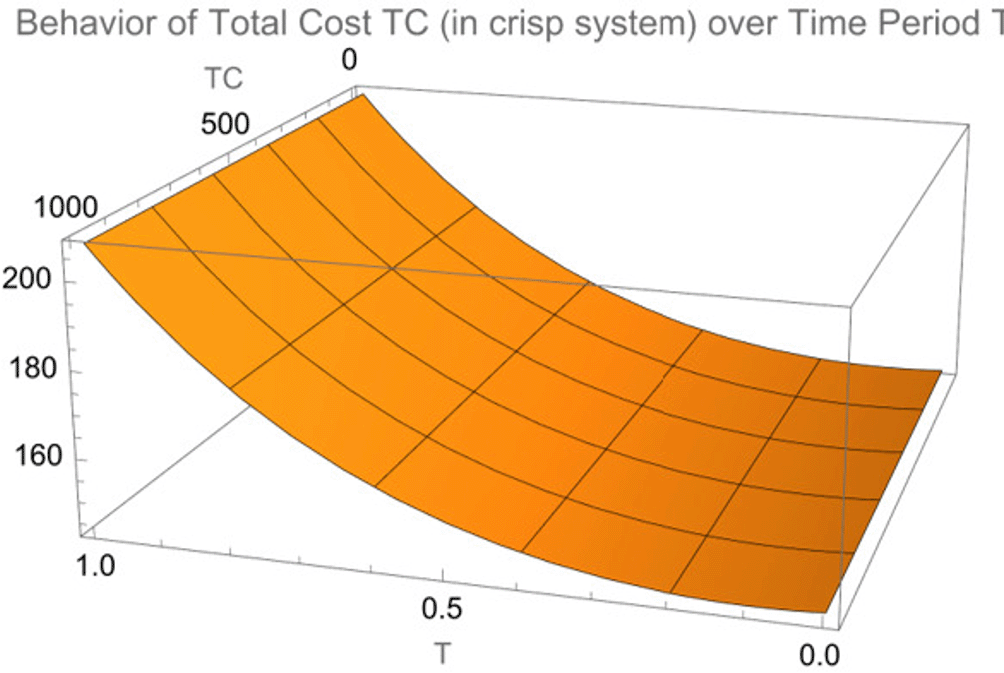
Figure 1. 3D plot of the total cost (TC) against the time period (T) for the Crisp inventory system.

The surface demonstrates how costs vary with time, showing that the Crisp model becomes more expensive over longer planning horizons.

Figure 2 is a 2D plot showing the behavior of the total cost (TC) over time period T, where the x-axis represents the time period and the y-axis represents the total cost.

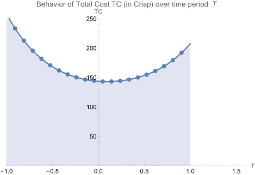
Figure 2. 2D plot of the total cost (TC) against the time period (T) for the Crisp inventory system.

The curve shows a nonlinear increase in cost over time, indicating that inventory costs accelerate as the cycle extends.

As shown in Figure 2, the total cost starts at a lower value and increases over time, indicating that the total cost accumulates as time progresses. However, the curve on the graph shows that the cost accelerates over time instead of increasing at a constant rate, as it is a nonlinear increase. We can say that the behavior of the curve implies that the initial costs are lower at the time being, but when time increases, additional costs contribute to an increase in the total cost.

12.2 Graphical analysis for fuzzy environment

Figure 3 on a 3D plot is showing the total cost (TC) over time period T in the fuzzy system. The x-axis represents the time period, y-axis represents the total cost, and z-axis represents another dimension of the total cost (TC) variation, which suggests additional factors that influence the cost (Toomey, 2000). Unlike the 2D graph, Figure 1 3D surface shows a decrease in the total cost over time. The surface indicates that as time increases, the system becomes more cost-effective, reducing the overall total cost.

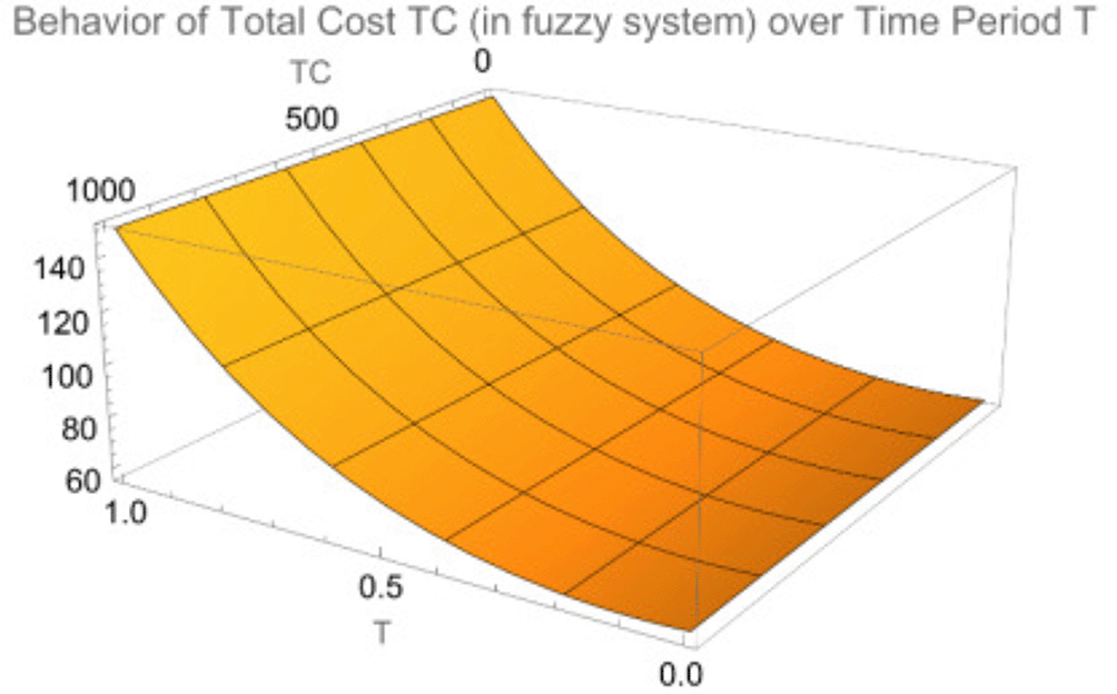
Figure 3. 3D plot of the total cost (TC) against the time period (T) for the Fuzzy inventory system.

The plot illustrates that the fuzzy system achieves lower costs and greater stability under uncertainty compared to the Crisp system.

Figure 4 is a 2D plot showing the behavior of the total cost (TC) over time period T, where the x-axis represents the time period and the y-axis represents the total cost.

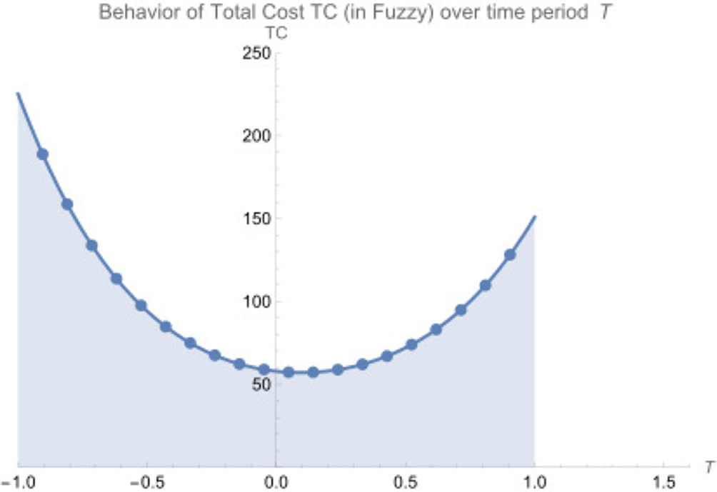
Figure 4. 2D plot of the total cost (TC) against the time period (T) for the Fuzzy inventory system.

The cost curve shows a slower, more controlled growth in costs over time compared to the Crisp model.

As shown in Figure 4, the total cost starts at a lower value and increases over time, indicating that the total cost accumulates as time progresses. However, the curve on the graph shows that the cost accelerates over time instead of increasing at a constant rate, as it is a nonlinear increase. We can say that the behavior of the curve implies that the initial costs are lower at the time being (SurveyMonkey, 2018), but when time increases, additional costs contribute to an increase in the total cost.

13. Conclusion

To conclude, this study developed a strong mathematical model designed to optimize inventory management strategies when dealing with fluctuating production rates and time-varying demand. Our findings highlight the significance of production-rate variability in influencing customer satisfaction and maximizing profitability. This model has emphasized the advantages of minimizing the initial stick accumulation, thereby reducing the holding costs and improving the overall operational efficiency (Roslin et al., 2015).

The sensitivity analysis demonstrated the model’s reliability and practical value, providing valuable information for decision-making in the industrial and retail industries (Sayal and Singh, 2022). To ensure accuracy and reliability of our suggestions, we used Mathematica 14.0. This study makes a significant contribution to the literature by providing a structured framework for determining the optimal order quantities, production durations, and inventory costs (Statistics Solutions, 2021). Business can refer to this framework to gain a competitive edge through more efficient supply chain management practices.

For future research purposes, we hope to extend our model to include additional factors such as dynamic market conditions and diverse demand rates, such as the Weibull distribution. This research is expected to provide stakeholders with the capacity to make knowledgeable decisions that can align production capabilities to market demands and, hence, promote profitable growth in the current competitive environment.

Ethical statement

The authors declare that all procedures followed in this study were conducted in accordance with ethical standards. The data used in this research were publicly available and anonymized to ensure that no personally identifiable information (PII) of the users was accessed or compromised. The authors have no conflicts of interest to disclose, and all the results have been reported transparently and without bias. Additionally, the research did not involve any human or animal subjects directly, and as such, did not require specific ethical approval from an institutional review board.

Data availability statement

No dataset is associated with this study. It is purely based on a numerical illustration, where the total cost has been calculated for both crisp and fuzzy systems. The study does not involve empirical data collection, and therefore no external dataset is available.

Extended data

No supplementary or extended data are associated with this study. All relevant mathematical derivations, equations, and numerical results are fully included within the manuscript.

References

Blundell R, Pashardes P, Weber G: What do we learn about consumer demand patterns from micro data? Am. Econ. Rev. 1993; 83(3): 570–597. Reference Source
CFI Team: EOQ. Corporate Finance Institute; 2023. Reference Source
Coker AK: Multiple linear regression – an overview. ScienceDirect Topics. n.d. Reference Source
Dhiman N, Sayal A: Optimization of inventory model for deteriorating items with time-varying holding cost under uncertainty. ResearchGate. 2022. Reference Source
Ebinesar MD: Different types of fuzzy numbers and certain properties. ResearchGate. 2015. Reference Source
Fleetwood D: Quantitative research: What it is, practices & methods. QuestionPro. 2018. Reference Source
Gnoni MG, Iavagnilio R, Mossa G, et al.: Modelling dynamics of a supply chain under uncertainty: a case from the automotive industry. Int. J. Automot. Technol. Manag. 2003; 3(3/4): 354–366. Publisher Full Text
Hagglund V: What are ordering costs? Understanding the fundamentals. ShipHero Blog; 2023. Reference Source
Ivanchenko IV, Ivanchenko D, Khruslov MM, et al.: Criteria of applicability of the resonant microwave method for measuring dielectric constants in the frequency band. Telecommunications and Radio Engineering. 2017; 76(18): 1661–1669. Publisher Full Text
Jaber MY: Inventory management: Non-classical view. ResearchGate. 2009. Reference Source
Kozarević S, Puška A: Use of fuzzy logic for measuring practices and performances of supply chain. Operations Research Perspectives. 2018; 5: 150–160. Publisher Full Text
Lutkevich B: What is a supply chain? Definition, models and best practices. TechTarget WhatIs.com. 2021. Reference Source
Maxwell M: Improving the Tesla master production schedule using AI/ML. ResearchGate. 2022. Publisher Full Text
Mondal R, Shaikh AA, Bhunia AK: Crisp and interval inventory models for ameliorating item with Weibull distributed amelioration and deterioration via quantum-behaved particle swarm optimization. Math. Comput. Model. Dyn. Syst. 2019; 25(6): 602–626. Publisher Full Text
Nima K: The effect of human learning and forgetting on fuzzy EOQ model with backorders. Universiti Utara Malaysia Repository. 2017. Reference Source
Olorunfemi B: The innovations driving Tesla’s success: Disruptions, customer transformation, and entrepreneurial strategies. Qeios. 2024; 1(1). Publisher Full Text
Olvera V, Segura E: Sensitivity analysis applied to a collaborative inventory model. International Joint Conference on Industrial Engineering and Operations Management. n.d. Reference Source
Park KS: Fuzzy-set theoretic interpretation of economic order quantity. IEEE Trans. Syst. Man Cybern. 1987; 17(6): 1082–1084. Publisher Full Text
Phair D, Warren K: Saunders’ research onion: Explained simply. Grad. Coach. 2021. Reference Source
PV R: Graphical analysis. Six Sigma Study Guide. 2014. Reference Source
Roslin E, Norhafiza S, Razak A, et al.: A conceptual model of inventory management system using an EOQ technique: A case study in automotive service industry. Journal of Science & Engineering Technology (JSET). 2015; 2: 1–10. Reference Source
Samanta B, Al-Araimi SA: An inventory control model using fuzzy logic. Int. J. Prod. Econ. 2001; 73(3): 217–226. Publisher Full Text
Sayal A, Dhiman N: Optimization of economic order quantity model with shortages having two-parameter Weibull demand and deterioration rate under crisp and fuzzy system. Int. J. Ind. Eng. Comput. 2022.
Sayal A, Singh AP: Optimized crisp and fuzzy inventory system of deteriorating items with partial backlogging under the effect of inflation. J. Ind. Prod. Eng. 2022.
Sayal A, Singh AP, Aggarwal D: Optimisation of EOQ model with Weibull deterioration under crisp and fuzzy environment. Int. J. Math. Oper. Res. 2019.
Sayal A, Singh AP, Aggarwal D: Inventory model in fuzzy environment without shortage using triangular fuzzy number with sensitivity analysis. Int. J. Manag. Sci. Eng. Manag. 2018. Reference Source
Singh J: Fuzzification and defuzzification. Scribd Presentation; n.d. Reference Source
Singh D, Alharbi M, Jayswal A, et al.: Analysis of inventory model for quadratic demand with three levels of production. Intelligent Automation & Soft Computing. 2022; 32(1): 167–182. Publisher Full Text
Solutions T: Inventory management: Importance and benefits. Tally Solutions. 2020. Reference Source
Square: Inventory management 101: How to manage small business inventory. SquareUp; 2021. Reference Source
Statistics Solutions: Pearson’s correlation coefficient. Statistics Solutions. 2021. Reference Source
SurveyMonkey: How to analyze survey data: Methods & examples. SurveyMonkey; 2018. Reference Source
Tally: Importance of inventory management: Definition & benefits. Tally Solutions; 2020. Reference Source
Toomey JW: Inventory management: Principles, concepts and techniques. Springer Science & Business Media; 2000. 978-1-4613-5701-3.
Wang JL: A supply chain application of fuzzy set theory to inventory control models – DRP system analysis. Expert Syst. Appl. 2009; 36(5): 9229–9239. Publisher Full Text
Yildiz H, DuHadway S, Narasimhan R, et al.: Production planning using evolving demand forecasts in the automotive industry. IEEE Trans. Eng. Manag. 2016; 63(3): 296–304. Publisher Full Text
Zarandi MH, Zarani MM, Saghiri S: Five crisp and fuzzy models for supply chain of an automotive manufacturing system. Int. J. Manag. Sci. Eng. Manag. 2007; 2(3): 178–196. Publisher Full Text

Comments on this article Comments (0)

Version 1

VERSION 1 PUBLISHED 28 Nov 2025

Author details Author details

¹ School of Accounting and Finance, Faculty of Business and Law, Taylor's University, Subang Jaya, Selangor, 47500, Malaysia
² College of Administrative and Financial Sciences, Saudi Electronic University, Riyadh, 11673, Saudi Arabia
³ Uttaranchal Institute of Management, Uttaranchal University, Dehradun, Uttarakhand, India

Anu Sayal
Roles: Conceptualization, Data Curation, Formal Analysis, Investigation, Methodology, Supervision, Validation, Writing – Original Draft Preparation, Writing – Review & Editing

Lai Yee Tong
Roles: Methodology, Resources, Software, Visualization, Writing – Original Draft Preparation

Amar Johri
Roles: Data Curation

Ashfaque Ahmed
Roles: Resources, Validation

Shahid Husain
Roles: Software

Seema Khurshid Qureshi
Roles: Visualization

Vasim Ahmad
Roles: Conceptualization

Competing interests

No competing interests were disclosed.

Grant information

The author(s) declared that no grants were involved in supporting this work.

Article Versions (1)

version 1

Published: 28 Nov 2025, 14:1330

https://doi.org/10.12688/f1000research.170276.1

Copyright

© 2025 Sayal A et al. This is an open access article distributed under the terms of the Creative Commons Attribution License, which permits unrestricted use, distribution, and reproduction in any medium, provided the original work is properly cited.

Download

Export To

metrics

	Views	Downloads
F1000Research	-	-
PubMed Central Data from PMC are received and updated monthly.	-	-

Citations

0

SEE MORE DETAILS

CITE

how to cite this article

Sayal A, Tong LY, Johri A et al. Optimizing inventory management in the automotive industry: A comparative study of crisp and fuzzy systems [version 1; peer review: awaiting peer review]. F1000Research 2025, 14:1330 (https://doi.org/10.12688/f1000research.170276.1)

NOTE: If applicable, it is important to ensure the information in square brackets after the title is included in all citations of this article.

track

receive updates on this article

Track an article to receive email alerts on any updates to this article.

Open Peer Review

Comments on this article Comments (0)

Version 1

VERSION 1 PUBLISHED 28 Nov 2025

Open Peer Review

Reviewer Status

AWAITING PEER REVIEW

Comments on this article

All Comments(0)

Add a comment

Sign up for content alerts

Browse by related subjects

[1] Blundell R, Pashardes P, Weber G: What do we learn about consumer demand patterns from micro data? Am. Econ. Rev. 1993; 83(3): 570–597. Reference Source

[2] CFI Team: EOQ. Corporate Finance Institute; 2023. Reference Source

[3] Coker AK: Multiple linear regression – an overview. ScienceDirect Topics. n.d. Reference Source

[4] Dhiman N, Sayal A: Optimization of inventory model for deteriorating items with time-varying holding cost under uncertainty. ResearchGate. 2022. Reference Source

[5] Ebinesar MD: Different types of fuzzy numbers and certain properties. ResearchGate. 2015. Reference Source

[6] Fleetwood D: Quantitative research: What it is, practices & methods. QuestionPro. 2018. Reference Source

[7] Gnoni MG, Iavagnilio R, Mossa G, et al.: Modelling dynamics of a supply chain under uncertainty: a case from the automotive industry. Int. J. Automot. Technol. Manag. 2003; 3(3/4): 354–366. Publisher Full Text

[8] Hagglund V: What are ordering costs? Understanding the fundamentals. ShipHero Blog; 2023. Reference Source

[9] Ivanchenko IV, Ivanchenko D, Khruslov MM, et al.: Criteria of applicability of the resonant microwave method for measuring dielectric constants in the frequency band. Telecommunications and Radio Engineering. 2017; 76(18): 1661–1669. Publisher Full Text

[10] Jaber MY: Inventory management: Non-classical view. ResearchGate. 2009. Reference Source

[11] Kozarević S, Puška A: Use of fuzzy logic for measuring practices and performances of supply chain. Operations Research Perspectives. 2018; 5: 150–160. Publisher Full Text

[12] Lutkevich B: What is a supply chain? Definition, models and best practices. TechTarget WhatIs.com. 2021. Reference Source

[13] Maxwell M: Improving the Tesla master production schedule using AI/ML. ResearchGate. 2022. Publisher Full Text

[14] Mondal R, Shaikh AA, Bhunia AK: Crisp and interval inventory models for ameliorating item with Weibull distributed amelioration and deterioration via quantum-behaved particle swarm optimization. Math. Comput. Model. Dyn. Syst. 2019; 25(6): 602–626. Publisher Full Text

[15] Nima K: The effect of human learning and forgetting on fuzzy EOQ model with backorders. Universiti Utara Malaysia Repository. 2017. Reference Source

[16] Olorunfemi B: The innovations driving Tesla’s success: Disruptions, customer transformation, and entrepreneurial strategies. Qeios. 2024; 1(1). Publisher Full Text

[17] Olvera V, Segura E: Sensitivity analysis applied to a collaborative inventory model. International Joint Conference on Industrial Engineering and Operations Management. n.d. Reference Source

[18] Park KS: Fuzzy-set theoretic interpretation of economic order quantity. IEEE Trans. Syst. Man Cybern. 1987; 17(6): 1082–1084. Publisher Full Text

[19] Phair D, Warren K: Saunders’ research onion: Explained simply. Grad. Coach. 2021. Reference Source

[20] PV R: Graphical analysis. Six Sigma Study Guide. 2014. Reference Source

[21] Roslin E, Norhafiza S, Razak A, et al.: A conceptual model of inventory management system using an EOQ technique: A case study in automotive service industry. Journal of Science & Engineering Technology (JSET). 2015; 2: 1–10. Reference Source

[22] Samanta B, Al-Araimi SA: An inventory control model using fuzzy logic. Int. J. Prod. Econ. 2001; 73(3): 217–226. Publisher Full Text

[23] Sayal A, Dhiman N: Optimization of economic order quantity model with shortages having two-parameter Weibull demand and deterioration rate under crisp and fuzzy system. Int. J. Ind. Eng. Comput. 2022.

[24] Sayal A, Singh AP: Optimized crisp and fuzzy inventory system of deteriorating items with partial backlogging under the effect of inflation. J. Ind. Prod. Eng. 2022.

[25] Sayal A, Singh AP, Aggarwal D: Optimisation of EOQ model with Weibull deterioration under crisp and fuzzy environment. Int. J. Math. Oper. Res. 2019.

[26] Sayal A, Singh AP, Aggarwal D: Inventory model in fuzzy environment without shortage using triangular fuzzy number with sensitivity analysis. Int. J. Manag. Sci. Eng. Manag. 2018. Reference Source

[27] Singh J: Fuzzification and defuzzification. Scribd Presentation; n.d. Reference Source

[28] Singh D, Alharbi M, Jayswal A, et al.: Analysis of inventory model for quadratic demand with three levels of production. Intelligent Automation & Soft Computing. 2022; 32(1): 167–182. Publisher Full Text

[29] Solutions T: Inventory management: Importance and benefits. Tally Solutions. 2020. Reference Source

[30] Square: Inventory management 101: How to manage small business inventory. SquareUp; 2021. Reference Source

[31] Statistics Solutions: Pearson’s correlation coefficient. Statistics Solutions. 2021. Reference Source

[32] SurveyMonkey: How to analyze survey data: Methods & examples. SurveyMonkey; 2018. Reference Source

[33] Tally: Importance of inventory management: Definition & benefits. Tally Solutions; 2020. Reference Source

[34] Toomey JW: Inventory management: Principles, concepts and techniques. Springer Science & Business Media; 2000. 978-1-4613-5701-3.

[35] Wang JL: A supply chain application of fuzzy set theory to inventory control models – DRP system analysis. Expert Syst. Appl. 2009; 36(5): 9229–9239. Publisher Full Text

[36] Yildiz H, DuHadway S, Narasimhan R, et al.: Production planning using evolving demand forecasts in the automotive industry. IEEE Trans. Eng. Manag. 2016; 63(3): 296–304. Publisher Full Text

[37] Zarandi MH, Zarani MM, Saghiri S: Five crisp and fuzzy models for supply chain of an automotive manufacturing system. Int. J. Manag. Sci. Eng. Manag. 2007; 2(3): 178–196. Publisher Full Text