Aerodynamic Drag Reduction in Commercial Vehicle Using CFD-Based Design Optimisation

Madhav S Prabhu; Sudheendra Prabhu K; Amar A Murthy; Srinivas G

doi:10.12688/f1000research.163917.1

Home Browse Aerodynamic Drag Reduction in Commercial Vehicle Using CFD-Based Design...

ALL Metrics

-

Views

-

Downloads

Get PDF

Get XML

Export

▬

✚

Research Article

Aerodynamic Drag Reduction in Commercial Vehicle Using CFD-Based Design Optimisation

[version 1; peer review: awaiting peer review]

Madhav S Prabhu¹, Sudheendra Prabhu K¹, Amar A Murthy², Srinivas G ¹

PUBLISHED 26 Aug 2025

Author details Author details

¹ Department of Aeronautical & Automobile Engineering, Manipal Institute of Technology (MIT), Manipal Academy of Higher Education (MAHE), Manipal, Udupi, Karnataka, 576104, India
² Department of Mechanical & Industrial Engineering, Manipal Institute of Technology (MIT), Manipal Academy of Higher Education (MAHE), Manipal, Udupi, Karnataka, 576104, India

Madhav S Prabhu
Roles: Conceptualization, Data Curation, Formal Analysis

Sudheendra Prabhu K
Roles: Funding Acquisition, Investigation, Methodology, Resources

Amar A Murthy
Roles: Investigation, Software, Writing – Original Draft Preparation

Srinivas G
Roles: Investigation, Methodology, Project Administration, Supervision, Writing – Review & Editing

OPEN PEER REVIEW

REVIEWER STATUS AWAITING PEER REVIEW

Abstract

Background

The aerodynamics of commercial vehicles is complex. The bluff body of a truck creates complex airflow patterns and induces drag. Numerous researchers have concentrated on enhancing the design of passenger cars, whereas the aerodynamic design of trucks has been largely overlooked. Truck operators are often unaware of the drag force acting on the truck and its impact on annual fuel consumption. Trucks can save large amounts of fuel annually by improving their aerodynamics. Most trucks are currently operating on the road without any frontal wind deflector, which causes drag accumulation over the frontal region of the truck.

Method

This study aims to reduce the drag force of an SCV through effective design optimization using the ANSYS Fluent tool. Using CFD methods and various numerical techniques, a comprehensive 3D airflow analysis was conducted on a scaled-down truck model. Subsequently, design optimizations were performed on the baseline truck to enhance its aerodynamic efficiency. A systematic literature review was conducted to obtain insights into the flow field of commercial vehicle drag-reduction techniques.

Results

Flow analysis was performed using different turbulence models, and the results were validated using available literature data. To improve the aerodynamic performance of the truck, different geometrical optimization models were tested on an iterative basis. Each model was further compared with the baseline model to obtain more reliable results. An airflow analysis was conducted for different air velocities. The obtained drag values for both the aerodynamically optimized truck and the baseline truck were compared and analyzed. Effective design alterations led to an 18% reduction in drag.

Conclusions

The enhanced aerodynamic outcomes are presented in detail for the optimized truck model. This study will help automobile engineers and truck researchers to understand the flow aerodynamics of commercial vehicles and improve their aerodynamic efficiency.

Keywords

Truck, CFD, Aerodynamics, Drag, Optimization, Flow control techniques

Corresponding author: Srinivas G

Competing interests: No competing interests were disclosed.

Grant information: The author(s) declared that no grants were involved in supporting this work.

Copyright: © 2025 Prabhu MS et al. This is an open access article distributed under the terms of the Creative Commons Attribution License, which permits unrestricted use, distribution, and reproduction in any medium, provided the original work is properly cited.

How to cite: Prabhu MS, Prabhu K S, Murthy AA and G S. Aerodynamic Drag Reduction in Commercial Vehicle Using CFD-Based Design Optimisation [version 1; peer review: awaiting peer review]. F1000Research 2025, 14:821 (https://doi.org/10.12688/f1000research.163917.1) First published: 26 Aug 2025, 14:821 (https://doi.org/10.12688/f1000research.163917.1) Latest published: 26 Aug 2025, 14:821 (https://doi.org/10.12688/f1000research.163917.1)

1. Introduction

Aerodynamics in automobile vehicle design plays a very important role, as they directly impact a vehicle's fuel efficiency and overall performance. By reducing the air resistance, vehicles can improve their fuel economy. An improved aerodynamic design reduces wind noise at higher speeds and enhances vehicle handling. Drag is classified into three main types: skin friction drag, induced drag, and form drag. Owing to the boxy shape of heavy commercial vehicles, truck vehicles experience more air resistance. A drag is a prominent force acting on a vehicle at higher speeds. Most trucks are not aerodynamically efficient, and by optimizing truck design, the fuel consumption can be reduced by up to 20%.¹ Modern automotive designs focus on vehicle frontal wind deflector designs and the streamlined shape of vehicles. An optimal design ensures smooth airflow around the vehicle body and reduces the overall drag force.

Commercial trucks are the backbone of the transport industry and play an essential role in supplying goods over long distances, in supply chains, and in logistics. The main advantages of commercial vehicles in the transport industry include their high load-carrying capacity and durability. Limited maneuverability in cities and other environmental concerns, such as high carbon emissions and high fuel consumption, are some limitations. The importance of aerodynamic design is a major topic for discussion. Drag arises mainly from vehicle shape, installing aerodynamic devices such as cab-side extenders and frontal wind deflectors will improve fuel economy and lower carbon emissions.

Figure 1 shows recent developments in truck design. Streamlining the truck body with various devices and a sleeker shape to reduce the resistance is the most common and effective method. Aerodynamic enhancements such as cab roof fairing and gap enclosures help minimize vehicle drag at highway speeds. Aerodynamic enhancements such as cab roof fairing and gap enclosures help minimize vehicle drag at highway speeds. Electric vehicles in the commercial category have also been developed and are emerging in many European countries. In terms of safety, top-model commercial vehicles in many European countries also include features such as cruise control and advanced lane-keeping assistance systems. Additional aerodynamic features, such as active grille shutters, are used for cooling engine components whenever needed. Overall, these innovations aim to reduce drag and improve truck performance, which helps the trucking industry reduce greenhouse gas emissions and align with global environmental sustainability goals.

Figure 1. Various aerodynamic devices installed on a heavy commercial vehicle.¹

2. Literature review

A systematic literature review was conducted in the field of vehicle drag reduction using wind-tunnel methods.^2–4 In summary, passive drag reduction strategies have shown significant potential for reducing aerodynamic drag. Simplified bluff bodies, such as the Ahmed body, are the most widely used vehicle models for research purposes,⁵ and have been used as benchmarks for different numerical and experimental studies. Techniques such as vortex generators,⁶ rear cavities, and devices such as fences or forward-facing panels can effectively reduce drag by controlling the airflow and delaying separation. For instance, small-scale wind tunnel tests have reported drag reductions exceeding 50% using drag-reduction methods. However, the drag reduction results from simplified models must be approached cautiously.^7,8 Simplified bodies can only offer approximate indicators of real-world performance. Future research must consistently verify the effects of drag reduction devices on fully detailed vehicles in actual driving scenarios.⁹

Similarly, a review of the literature on numerical methods was performed, focusing on various turbulence models. The use of diverse numerical techniques for analyzing the flow remains essential for understanding the flow characteristics of a vehicle. The comparison of drag suggests that realizable K-epsilon provides greater accuracy than DDES.¹⁰ LES is a reliable method for studying various aerodynamic loads and is highly effective under different conditions. To analyze the flow around the truck model, utilizing turbulence models such as the realizable k-ε and k-omega SST in the ANSYS solver will yield more accurate outcomes.¹¹ Implementing these models will significantly decrease the computational cost, with the realizable k–ε model giving the closest value to the experimental data and with the least error. Hybrid RANS/LES models have proven to be more effective than the RANS turbulence model in predicting the flow over vehicles, while still maintaining reasonable computational costs.^12,13 Comparisons of the drag indicate that the realizable k–ε model is more precise than the SST and DDES/SST models. The utilization of the DNS method in captures all turbulence scales, giving highly accurate results, although it incurs high computational costs.¹⁴ The selection of DNS, RANS, and LES techniques depends on the specific research type, available computational resources, and the desired level of result accuracy.

2.1 Research gaps

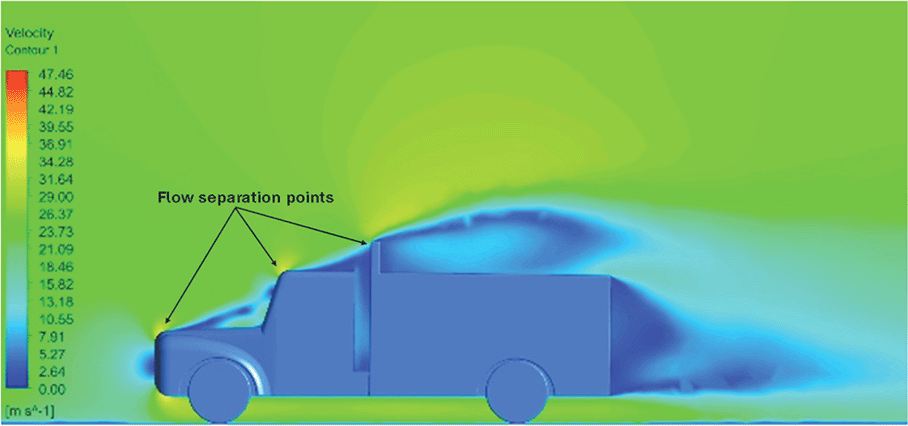
There are some limitations in the current research on 3D flow simulations for commercial trucks because of their complex body shapes. Because of the complex airflow patterns, greater computational resources are required to analyze the flow behavior. Although simplified models have been used to study small-scale vortices and turbulent wakes, full-scale simulations are crucial for understanding airflow interactions, especially under varying speeds. Underbody flow, including interactions between the rotating wheels and the ground, remains underexplored. Additionally, research on grid resolution, prism layer configurations, and turbulence models for commercial vehicles is insufficient compared to that for passenger cars.¹⁵ Flow separation points, particularly at the rear of the truck, produce complex wake patterns that are often oversimplified in various studies. Key aerodynamic factors such as temperature, density, velocity, and turbulence have also not been thoroughly analyzed.¹⁶ Addressing these gaps through full 3D simulations and improved numerical methods is essential for optimizing truck aerodynamics.

2.2 Research objectives

The objectives of the research are:

• To conduct an aerodynamic flow analysis of the truck and validate the results with experimental and numerical literature data.
• To investigate the aerodynamic flow performance parameters of a truck vehicle by incorporating various numerical techniques.

3. Methodology

Figure 2 shows the flowchart of the study. The process begins with an introduction to vehicle aerodynamics and a comprehensive literature review on drag reduction methods, in which existing studies are explored to gather important insights. A summary of the literature review helps identify gaps in the current research field. After defining the objectives, a baseline analysis was performed, and the truck model used for the analysis was a Bedford J-series light commercial vehicle.¹⁷ The computational fluid dynamics method is used, where numerical analysis focuses on various factors that affect aerodynamic behavior. Varying the turbulence models, inlet boundary conditions, and geometrical features of the vehicle helps to understand how different conditions and design modifications impact the overall flow field and drag reduction. Once the simulations were conducted, the results were evaluated to determine whether the required level of accuracy was obtained. If not, the truck design will be redesigned, and the final optimized model and simulation results are presented in this paper.

Figure 2. Methodology flowchart.

3.1 Baseline analysis

3.1.1 Modelling

In this study, CFD analysis was performed on a Bedford J Series truck model, chosen because of the easy availability of its blueprints, which facilitated the creation of a 3D model. In addition, this truck model is widely used in small commercial vehicle segments and is available in almost all countries. An experimental study was conducted using a similar model that focuses on drag reduction. Hence, the experimental data are publicly available to verify the accuracy of the CFD results.

The baseline model was a 1/10^th scaled-down model of the actual truck dimensions. Reference paper¹⁸ experiments on similar scaled-down models. Hence, in this work, similar dimensions were used for modeling the truck using ANSYS DesignModeler, and the experimental data were publicly available to check the accuracy of the CFD results. The baseline dimensions of the truck geometry are presented in Table 1.

Table 1. Truck model dimensions (1/10^th scale).¹⁷

Length (L)	0.57 m
Height (H)	0.25 m
Width (W)	0.22 m
Wheelbase (WB)	0.37 m
Truck Cabin-Trailer Gap (G)	0.02 m
Ground Clearance (GC)	0.035 m

Figures 3 and 4 show the 3D models of the scaled-down Bedford J-series truck. The ANSYS DesignModeler and SpaceClaim tools have been extensively used for 3D modeling.

Figure 3. Bedford truck 3D model (Side view).

Figure 4. Bedford truck 3D model (Front view).

Figure 5 shows blueprints of the Bedford truck. The dimensions of the reference paper were the same as the actual size. For this simulation, the actual dimensions were scaled to a factor of 10.

Figure 5. Blueprint of the Bedford J series truck.¹⁷

3.1.2 Meshing

The mesh was generated using ANSYS meshing module. For the initial meshing, a tetrahedral mesh was implemented, consisting of 6.2 million elements and 1.8 million nodes. An unstructured tetrahedral mesh is typically used for analyzing turbulent flows. Regarding the mesh quality, the average element quality was 0.73, while the maximum skewness value was 0.92. An orthogonal quality of 0.99 was obtained, with an average of 0.76. The named selections, surface mesh size, and other mesh details are listed in Table 2.

Table 2. Mesh details for the truck and enclosure.

Geometry	Selection type	Mesh details
Outer Domain	Body	18.5 – 21.5 mm
Truck Surface	Named Selection – Face Sizing	1.5 – 3 mm
Truck Surface	Named Selection – Inflation First Layer Thickness	0.35 mm
	Number of Layers (N)	5
	Growth Rate	1.2

Figure 6 shows the complete mesh generated in the ANSYS mesh module. The mesh size was set to 20 mm, whereas for the truck surface, it was set to 3 mm. The growth rate for the inflation layer was set to a default of 1.2, and the first layer thickness height was set to 0.3 mm with a maximum number of five layers to capture the boundary layer.

Figure 6. Mesh generated for the enclosure and the truck surface.

3.1.3 Boundary condition

After modeling the truck, a computational fluid domain that encompasses the truck model was established to simulate the airflow around the truck. The volume was established by subtracting the truck body using the Boolean function in DesignModeler. The truck length was six times the rear wall, two times the truck length to the front wall, two times the width of the truck to the side walls, and three times the truck height to the top wall. The boundary conditions used for the domain are shown in Figure 7, and the boundary conditions are listed in Table 3.

Figure 7. Computational fluid domain dimensions and boundary conditions.

Table 3. Boundary conditions for the named selections.

Named selection	Boundary type
Inlet	Velocity -Inlet
Outlet	Pressure -Outlet
Exterior Walls	Symmetry
Road	No-Slip Wall condition
Truck Surface	No-Slip Wall condition

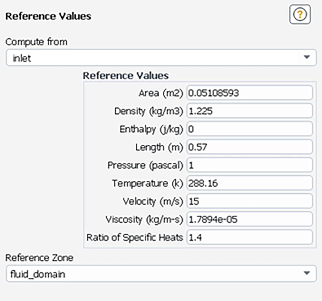
The solver was set up according to the model type and operating conditions. Operating conditions, such as atmospheric pressure for the truck at sea level, were assumed. The solver uses a pressure-based incompressible steady-state flow condition. Figure 8 shows the settings for the turbulence model, where the K-Epsilon (2 Equation) model was used, and the fluid properties of air were constant with a density of 1.225 kg/m³ ( Table 4).

Figure 8. Turbulence model settings and solution methods.

Table 4. Results of grid independence test.

Mesh size (mm)	Number of elements (million)	Drag coefficient (C_D)
21.5	6.01	0.476
21	6.11	0.533
20	6.23	0.547
19	6.38	0.551
18.5	6.47	0.554

The Standard K-Epsilon model with standard wall functions was used, and the semi-implicit method for pressure-linked equations (SIMPLE) algorithm was used as the pressure-velocity coupling scheme. The details of the solution method are shown in Figure 8 and Figure 9 shows the reference values used for the solution. The reference area was calculated for the projected frontal area of the truck, and the reference length was scaled down by the truck length.

Figure 9. Reference values.

3.1.4 Governing equations

Fluent software solves these Navier-Stokes equations, composed of the continuity equation and momentum equations, as given below (1) – (4).¹⁹

Continuity equation:

(1)

\frac{∂u}{∂x} + \frac{∂v}{∂y} + \frac{∂w}{∂z} = 0

X-Momentum equation:

(2)

ρ \frac{Du}{Dt} = - \frac{∂p}{\partial x} + μ (\frac{\partial^{2} u}{\partial x^{2}} + \frac{\partial^{2} u}{\partial y^{2}} + \frac{\partial^{2} u}{\partial z^{2}}) + ρ . f_{x}

Y-Momentum equation:

(3)

ρ \frac{Dv}{Dt} = - \frac{∂p}{\partial y} + μ (\frac{\partial^{2} v}{\partial x^{2}} + \frac{\partial^{2} v}{\partial y^{2}} + \frac{\partial^{2} v}{\partial z^{2}}) + ρ . f_{y}

Z-Momentum equation:

(4)

ρ \frac{Dw}{Dt} = - \frac{∂p}{\partial z} + μ (\frac{\partial^{2} w}{\partial x^{2}} + \frac{\partial^{2} w}{\partial y^{2}} + \frac{\partial^{2} w}{\partial z^{2}}) + ρ . f_{z}

Reynolds equation:

(5)

R_{e} = \frac{ρ . v . L}{μ}

The Reynolds number is a dimensionless value that determines whether the fluid flow is laminar or turbulent or not. Equation (5) represents the Reynolds number, where ρ is the fluid density (kg/m³), v is the fluid velocity (m/s), L is the characteristic length of the object (m), and μ is the dynamic viscosity of the fluid (kg/ms). The drag coefficient is represented in the simulations as a dimensionless value, illustrating the aerodynamic characteristics of the truck based on Equation (6).²⁰

(6)

C_{D} = \frac{F_{D}}{0.5 ρ A v^{2}}

where C_D = Drag coefficient, F_D = Drag force (N), ρ is the fluid density (kg/m³), A = Area (m²), and v = Velocity (m/s).

3.1.5 Drag coefficient plot

The simulation used the first-order upwind turbulent kinetic energy method. The report definition was used to calculate the drag coefficient (C_D) for the truck surface. Figure 10 shows the C_D plot of the simulation results.

Figure 10. Drag coefficient plot for baseline model.

4. Results and discussions

A grid independence test was performed for baseline model analysis to ensure an optimal mesh. Various turbulence models were tested to determine the best grid size, and the obtained results were analyzed. A varying velocity test was performed for the best turbulence model, and the effect of varying the velocity on the drag coefficient value was observed and studied.

4.1 Grid independence test

A grid independence test was conducted to ensure that the obtained drag coefficient results did not depend on the grid used in the simulation. Five different mesh sizes were chosen: 6.0, 6.1, 6.2, 6.3 and 6.4 million mesh elements. The five simulation results showed that the mesh sizes of 6.2, 6.3, 6.4 million elements had the same drag value of C_D = 0.55. Hence, a 20 mm mesh size with 6.2 million elements was chosen for further simulation. The error percentages for 6.2, 6.3, 6.4 million elements were similar. This ensured an optimal mesh was used for further simulations.

From Figure 11, it can be observed that the drag coefficient value remains constant at 6.2, 6.3 and 6.4 million elements. This ensured an optimal mesh was used for further simulations. The baseline mesh was set to 20 mm with 6.2 million mesh elements. The percentage error was obtained for the grid analysis.

Figure 11. Number of elements vs drag coefficient for baseline model.

4.2 Varying turbulence models

The model comparison results provided the best viscous model for further simulation, ensuring an accurate result with the least computational error. The drag coefficient value was compared with that in the reference paper.¹⁸

Figure 12 shows the turbulence model test results for the baseline model. To study how the results varied for different models, six different models were used in this simulation. The obtained drag coefficient values for the different models in Table 5 were compared with the experimental drag coefficient in the previous study.¹⁸ The Reynolds stress and K-Epsilon Standard models resulted in the lowest drag coefficient values.

Figure 12. Turbulence model performance vs C_D for the best grid size.

Table 5. Turbulence model comparison results.

Viscous models	Obtained Drag coefficient (C_D)	Experimental (C_D) Reference value¹⁸	Error (%)
Spalart Allmaras	0.51	0.47	8.51
K-Epsilon	0.49		4.25
SST K-Omega	0.55		17.02
Transition K-KL-Omega	0.59		25.53
Transition SST	0.53		12.76
Reynolds Stress	0.46		2.12

From Table 5, it can be observed that the Transition K-KL-Omega model resulted in a higher drag coefficient than the other models. The K-epsilon and Reynolds stress models had minimum drag values of C_D = 0.49 and C_D = 0.46, respectively, with the least error when compared with the experimental data. A comparison of the K-epsilon and Reynolds stress results will provide the best model for the final simulation.

Above Tables 6-8, shows the flow contours and streamlines of the baseline truck for six different turbulence models compared with the reference results. Tables 9 and 10 compare the contour results of the best turbulence model.

Table 6. Comparison of velocity contour and streamline contour of reference paper result with different viscous model results.¹⁸

Results	Reference paper results¹⁸	K-Epsilon model	Reynolds stress model
Velocity contour	The contour shows a single flow separation point with a large low velocity high pressure wake region. The Red points indicate a high velocity region near the front hood and cabins leading edge.	The velocity contour of K-Epsilon model shows a small low velocity region above the truck surface.	The velocity contour of this model shows a large disrupted low velocity region above the truck surface.
Velocity streamline	The reference paper streamlines show a large single circulating region above the truck. These regions contain small recirculating vortices which induce to drag.	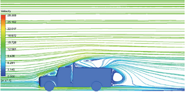The streamlines obtained shows a small recirculating region between the cabin trailer Gap, small vortex formation occur at these gaps.	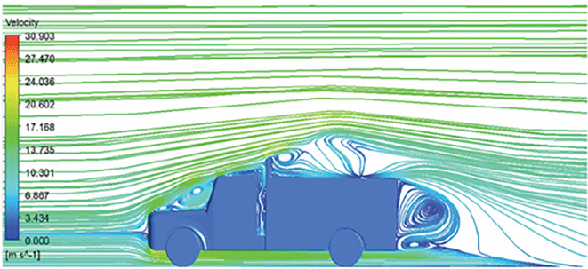The streamlines are more detailed, three large recirculating vortices are formed. The Reynolds stress model has the best streamline compared to all other models.

Table 7. Comparison of velocity contour and streamline contour of reference paper result with different viscous model results.¹⁸

Results	Reference paper results¹⁸	Spalart Allmaras model	Transition SST model
Velocity contour	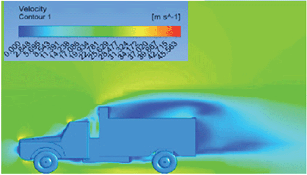The contour shows a single flow separation point with a large low velocity high pressure wake region. The Red points indicate a high velocity region near the front hood and cabins leading edge.	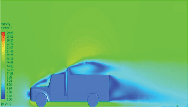The velocity contour of Spalart Allmaras model shows a higher wake region above the truck surface.	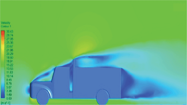The above velocity contour shows an abrupt flow separation point near the leading edge of the trailer.
Velocity streamline	The reference paper streamlines show a large single circulating region above the truck. These regions contain small recirculating vortices which induce to drag.	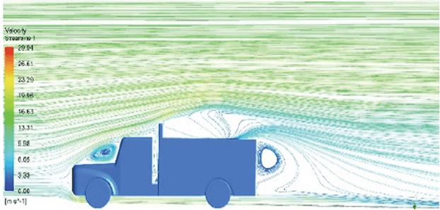The streamlines show a large recirculating region at the front region near the windshield.	Two tiny vortices are formed in the gap region of the truck. The flow reattachment occurs far away.

Table 8. Comparison of velocity contour and streamline contour of reference paper result with different viscous model results.¹⁸

Results	Reference paper results¹⁸	SST K-Omega model	Transition K-KL-Omega
Velocity contour	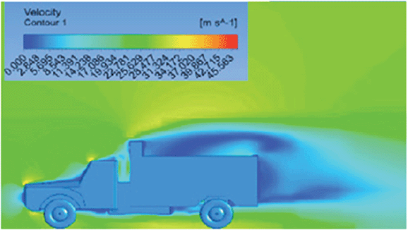The contour shows a single flow separation point with a large low velocity high pressure wake region. The Red points indicate a high velocity region near the front hood and cabins leading edge.	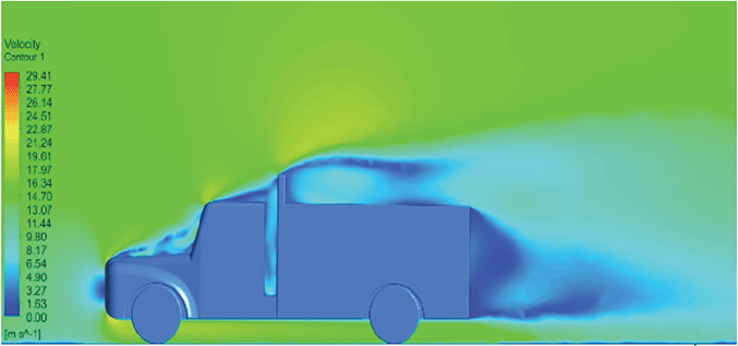Abrupt air flow profile is observed near the frontal hood	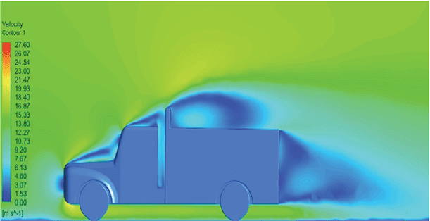A high air velocity points are observed near the edges.
Velocity streamline	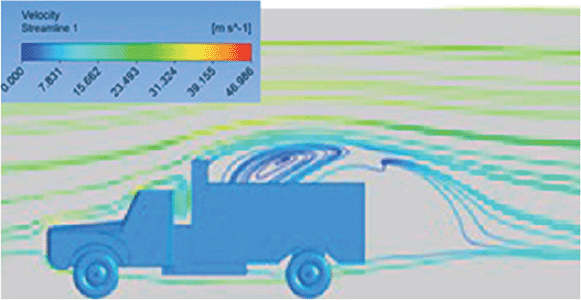The reference paper streamlines show a large single circulating region above the truck. These regions contain small recirculating vortices which induce to drag.	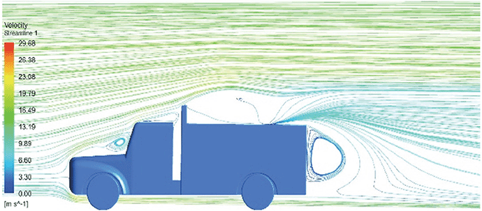The streamlines obtained shows a small recirculating region at the front region near the windshield.	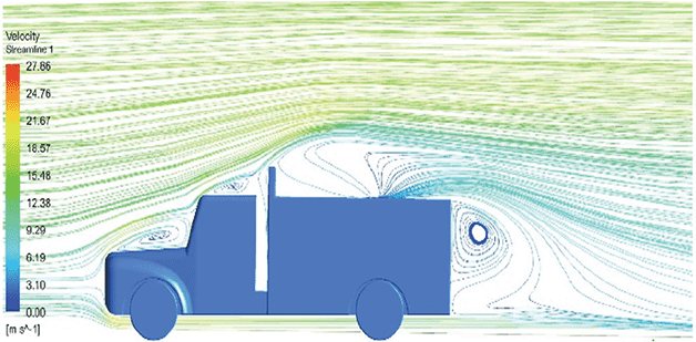The streamlines obtained shows a large recirculating vortex at the rear end of the truck.

Table 9. Comparison of velocity contours.

Model	Velocity contour plot	Remarks
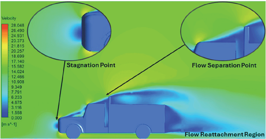
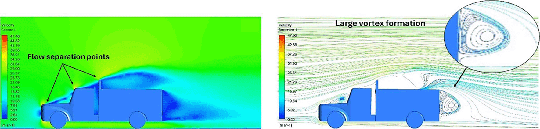
K-Epsilon Standard	Figure 13: K-Epsilon model velocity contour.	A stagnation point at the front of the truck is observed. At this region the air velocity is zero and the pressure is at its maximum. A lower wake region is observed at the top of the truck. Flow separation points are clearly visible near the truck cabins leading edge.
Reynolds Stress	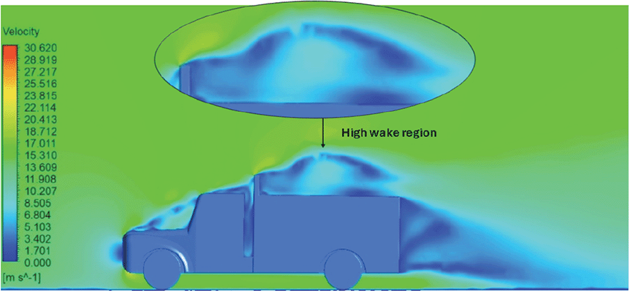Figure 14: Reynolds Stress model velocity contour	Similar stagnation point is observed near front region of the truck. The low air velocity with a high-pressure wake region is much bigger in size due to bluff body, and an abrupt flow separation region is observed at the top of the truck.

Table 10. Comparison of velocity streamlines.

Model	Velocity streamline	Remarks
K-Epsilon Standard	Figure 15: K-Epsilon model velocity streamline.	The detailed flow streamlines are obtained. The flow bubble near the gap between hood and windshield are visible. The recirculation in the gap region is prominent. Small vortex formations are observed near truck cabin.
Reynolds Stress	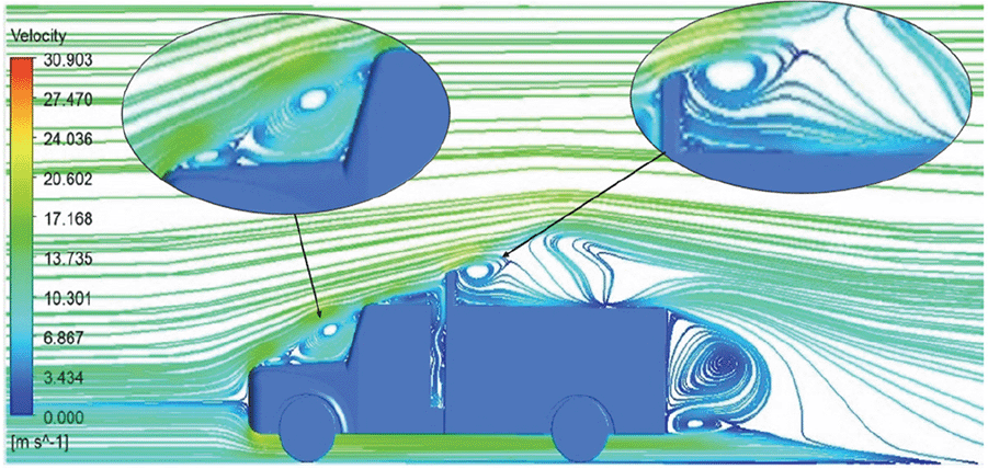Figure 16: Reynolds Stress model velocity streamline.	This model yielded the best detailed streamlines. The small vortex formation near the hood is clearly visible. In the rear wake region both large and small vortex was captured. This streamline plot provides better flow visuals when compared to other models.

The velocity streamlines in Figures 13 and 14 show the areas of flow recirculation of the K-epsilon and Reynolds stress models, respectively.

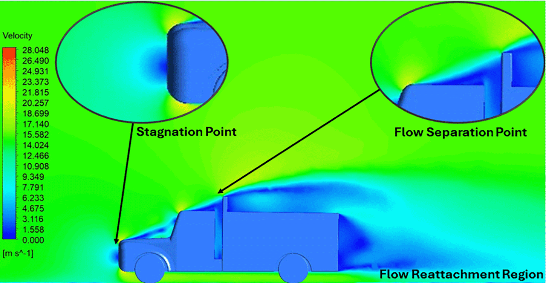
Figure 13. K-Epsilon model velocity contour.

Figure 14. Reynolds stress model velocity contour.

A significant area of flow recirculation is located at the back of the truck. Both large and small vortices were generated at these locations. The space between the cabin and the trailer produced a small flow recirculation area.

Introducing a gap enclosure allows air to flow from the sides of the truck cabin instead of flowing between the gaps. The underbody airflow is smooth in this case, and the vortex bubble formation near the front hood and cabin windshield is mainly caused by the angle between the hood and windshield ( Figures 15 and 16)

Figure 15. K-Epsilon model velocity streamline.

Figure 16. Reynolds stress model velocity streamline.

.

In conclusion, both of the above models resulted in accurate solutions and detailed streamlines. Considering the computational accuracy and cost, the K-epsilon (2 equation) model is much more efficient than the Reynolds Stress (7 equation) model.

The K-epsilon model is recognized for delivering precise outcomes under free-flow conditions, and this model results in faster solution convergence. Hence, The K-Epsilon Standard model was selected for the final simulation.

4.3 Varying inlet velocity

The inlet air velocities were varied to understand the variation in drag coefficient. As the vehicle speed increases, the drag also increases. The air velocity variation ranged from 40 to 90 km/h in the simulation with a 10 km/h increment. As the inlet air velocity increased, the drag coefficient also increased significantly.

From Table 11, it can be observed that for the velocity of 40 kmph (11.11 m/s) the drag coefficient value is 0.49 and for the maximum velocity, the drag coefficient is more than 1. Owing to the bluff body, the drag coefficient of a heavy truck vehicle was approximately 0.8. In this simulation, considering a highway operating speed of 70 km/h for a commercial truck, the drag coefficient obtained was C_D = 0.92.

Table 11. Values of drag coefficient for different air velocity.

Velocity (Kmph)	Drag coefficient (C_D)
40	0.49
50	0.50
60	0.68
70	0.72
80	0.92
90	1.20

From Figure 17, it can be observed that for an economical speed of 40-50 kmph, the drag values are minimal. As the speed increased, the drag suddenly increased. The highway operating speed of a truck is 70-80 kmph. At this speed, the fuel consumption is very high, and minimizing the overall drag experienced by the truck will help reduce fuel consumption. The overall drag coefficient was significantly higher in this case. At the maximum operating speed of the truck, the drag value exceeded 1, which is uncommon. Hence, by streamlining the body of the truck, a lower drag coefficient can be obtained. Generally, the drag value for these trucks is approximately 0.8.

Figure 17. Varying velocity vs drag coefficient for baseline truck model.

Figures 18 and 19 show the velocity contours and streamlines for the maximum and minimum air velocities, respectively, from this simulation. Similar flow contours were obtained for two large wake regions near the rear end of the truck.

Figure 18. Velocity contour and velocity streamline at 40 Kmph.

Figure 19. Velocity contour and velocity streamline at 90 Kmph.

4.4 Baseline model comparison and validation

The velocity contours and streamlines were compared with respect to the reference paper. A similar flow contour was obtained for the baseline truck analysis, and the results were satisfactory. The obtained drag coefficient value was closer to the experimental data, with the least error. Results were obtained and studied by varying the inlet boundary conditions. Finally, the K-epsilon model was selected as the best turbulence model.

In Figure 20, The baseline model data are plotted in blue in Figure 20. The overall drag coefficient for varying speeds was approximately C_D = 0.7. The comparison graph in Figure 21 shows the variation in drag values for different air speeds between the two models.

Figure 20. Drag coefficient (C_D) as a function of wind speed.¹⁸

Figure 21. Drag coefficient (C_D) vs varying velocity, comparison of reference paper¹⁸ model and present work baseline truck model results.

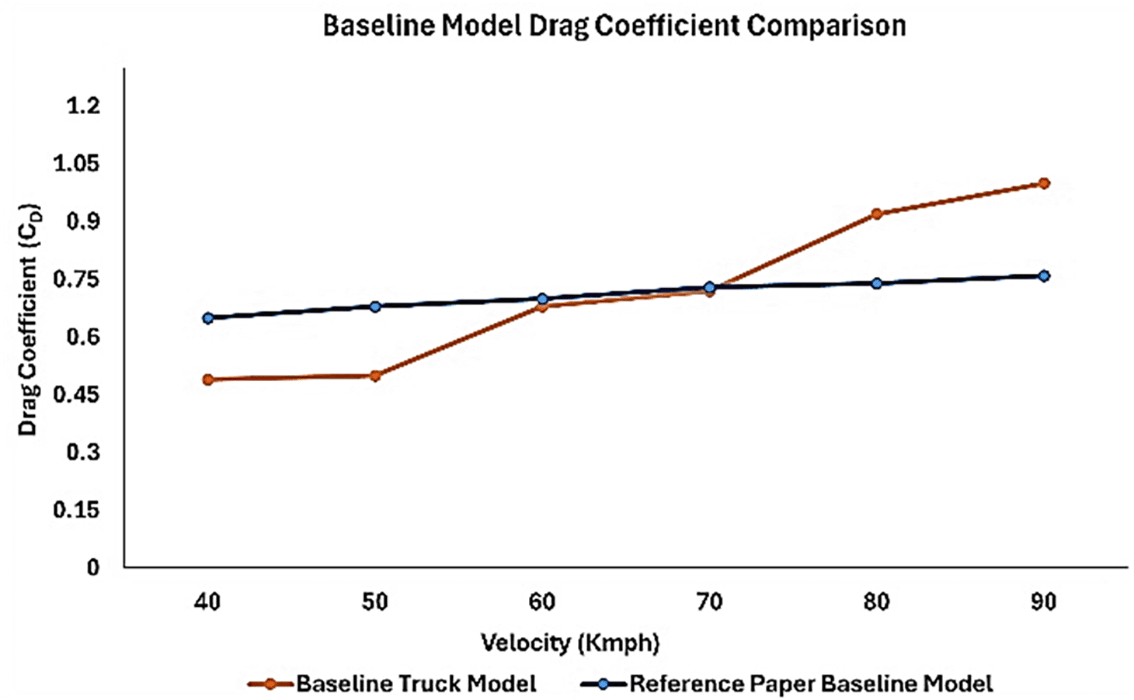
From Figure 21, it can be observed that for wind speeds of 70 km/h and above, the drag coefficient value increases significantly for the baseline model (orange line) in the present work. The reference paper baseline model drag (C_D) value is between 0.6 and 0.75. The overall drag coefficient value was less than that of the present work. In Figure 20, for the aerodynamically optimized truck model, the graph shows an overall drag coefficient value between 0.45 and 0.55. In the experimental reference paper, the installation of aerodynamic fairing is very effective, as the result shows a 12% reduction in drag forces compared to the baseline model.¹⁸ Because detailed values for the drag coefficient are not provided in the experimental reference paper, by referring to Figure 20, the drag values between 0.6 the purposes considered for comparison and validation purposes. The aim of this study is to improve aerodynamic efficiency.

The minimum error obtained by comparing the reference paper result and the present simulation paper result for an average speed of 60 km/h was 2.86%. The baseline model results were accurate, and the obtained drag value was closer to the experimental reference value.¹⁸

4.5 Optimised model analysis

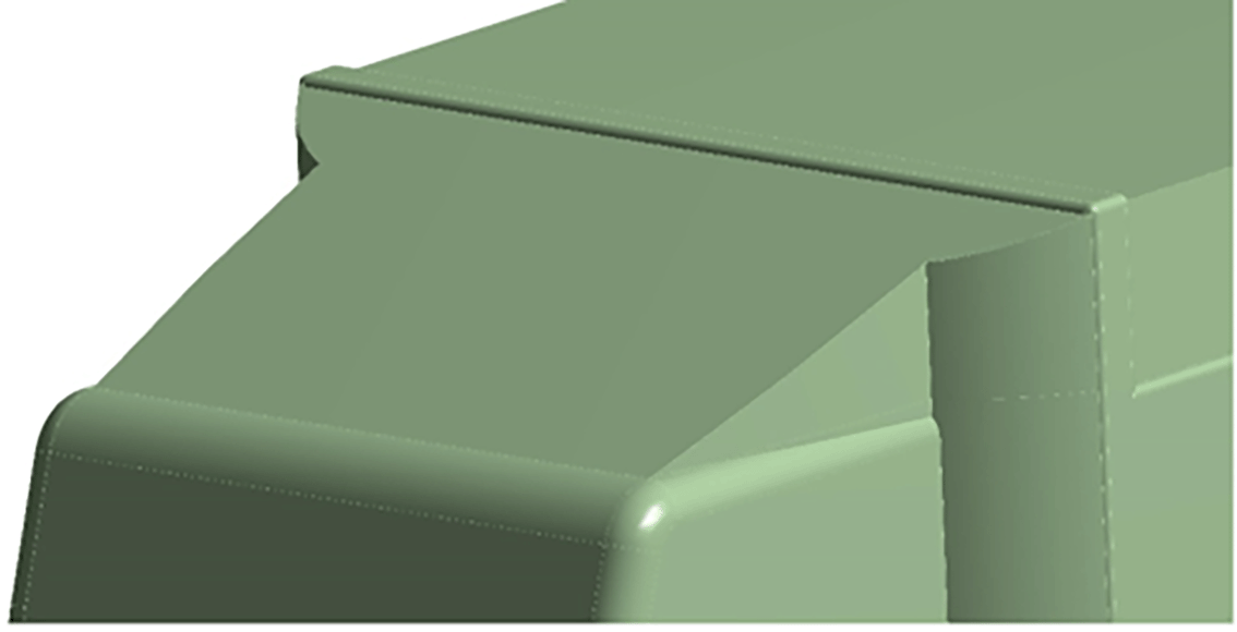
The Baseline truck model was redesigned, as shown in Figure 22, with a total of three design modifications: CRF was fitted to the cabin roof, a gap enclosure was added, which was then combined with CRF, and the square back was modified with an optimal slant angle. Various CRF angles were analyzed, and the best CRF angle was chosen for the final simulation. Similarly, various square-back slant angles were analyzed, and the best slant angle model was chosen. Finally, the best aerodynamically optimized truck design was presented.

Figure 22. Various CRF and square back design modifications for the baseline truck.

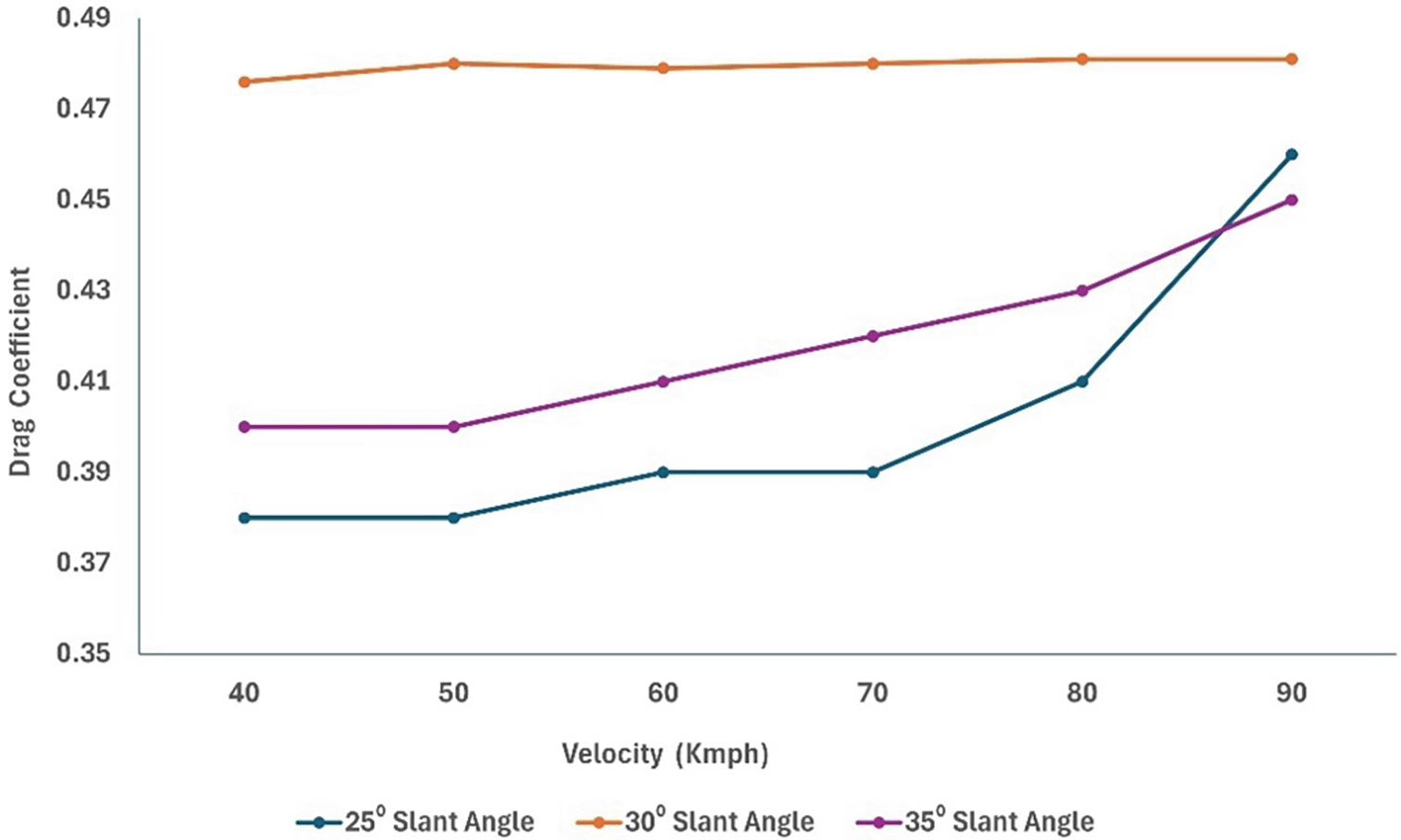
For the rear square-back modifications of the truck, three different slant angles with 5° variation for the square-back were used for the analysis.

For each modification, a grid-independence test was conducted to ensure that an optimal mesh was obtained. For the best grid size, various turbulence models were tested, and for the best model with the least computational error, a final simulation with varying air velocity was conducted. The results of all optimizations were then compared to obtain the best model. Finally, an aerodynamically optimized truck model is presented.

Figures 23 and 24 show the 3D models of the optimized truck. The truck’s geometrical dimensions are the same as those of the baseline, as given in Table 1. The dimensions of the CRF, Gap enclosure, and squareback for all modifications are listed in Tables 12, 13, and 14, respectively.

Figure 23. Optimised truck model (Isometric view).

Figure 24. Optimised truck model (Side view).

Table 12. CRF model dimensions.

Model 1 α = 25° W1 = 0.1457 m W2 = 0.1590 m X = 0.088 m X1 = 0.025 m Y = 0.04 m
Model 2 α = 20° W1 = 0.1457 m W2 = 0.1590 m X = 0.11063 m Y = 0.04 m
Model 3 α = 15° W1 = 0.1457 m W2 = 1590 m X = 0.11063 m Y = 0.04 m

Table 13. Gap fairing dimensions (1/10^th scale).

Gap Enclosure Length

L1 = 0.025 m

L2 = 0.025 m

Table 14. Square back modification dimensions (1/10^th scale).

25° Slant angle	β = 25°, Y = 0.04 m, L1 = 0.3 m, L2 = 0.2107 m, L3 = 0.0900 m
30° Slant angle	β = 30°, Y = 0.04 m, L1 = 0.3 m, L2 = 0.2323 m, L3 = 0.0718 m
35° Slant angle	β = 35°, Y = 0.04 m, L1 = 0.3 m, L2 = 0.2382 m, L3 = 0.0670 m

4.5.1 Cab roof fairing geometry

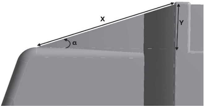
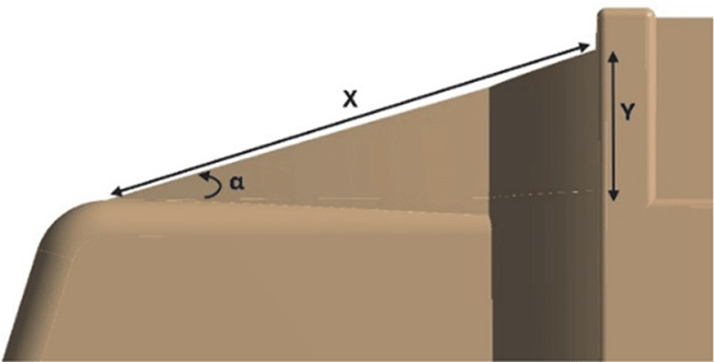
Aerodynamic devices, such as frontal wind deflectors and gap fairings, are fixed devices that do not require external power to operate and are known as passive drag reduction devices. These are the most effective devices for bluff bodies, such as trucks. These wind deflectors, commonly known as ‘Cab Roof Fairing’ (CRF), help the vehicle move smoothly through the air by redirecting the airflow around the vehicle. At higher speeds, these devices improve vehicle stability and reduce the side force under crosswind conditions.⁷ Similar studies were conducted using different CRF designs.

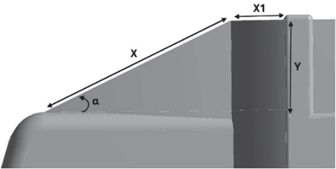
Figure 25 shows the optimized CRF attached to the truck cabin. Three different CRF models with different frontal angles were modelled. The CRF geometry was modelled using the ANSYS DesignModeler software and was attached to the baseline truck model cabin.

Figure 25. CRF attached with truck cabin and gap enclosure.

4.5.2 Gap fairing geometry

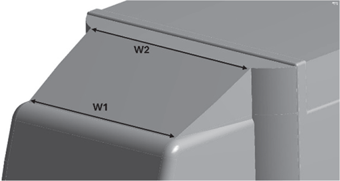
Additionally, to reduce flow recirculation in the gap between the truck cabin and goods trailer, a gap fairing was designed and combined with the CRF. The combination of CRF and gap farming ensures an optimal frontal design and enhances the appearance of trucks. For a truck cabin-trailer gap of 0.02 m, the gap enclosure was designed to avoid recirculating airflows. The dimensions are presented in Table 13.

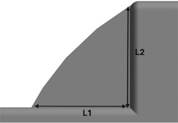
4.5.3 Square back geometry

Figure 26 shows the squareback modifications. The squareback modifications were inspired by the Ahmed Body squareback model. The Ahmed Body model is the most widely used model in the research field. In this study,²¹ a study on simplified three-dimensional square back Ahmed model was developed. This study signifies the importance of the slant angle (β), where β = 30° is known as the critical angle. Many researchers have conducted experimental and numerical analyses on the Ahmed model. The aim was to maintain airflow close to the body to achieve a minimal wake zone.

Figure 26. Square back geometry (Side view).

Figure 27 shows a simplified three-dimensional squareback Ahmed model. The current model demonstrated significant success in flow modification, with the angle adjusted between 25° and 35°. A Grid independence test was performed for all simulations, along with the evaluation of different turbulence models. The optimal model was then used to analyze the results due to changes in air velocity. Ultimately, the slant angle that minimized the overall drag was selected as the final model. The flow contours associated with each modification were thoroughly examined and analyzed.

Figure 27. Simplified three-dimensional square back Ahmed model.²¹

4.5.4 Optimised model results

After performing the grid analysis for each modification, the best grid was chosen for turbulence model testing. From Table 15 ( Figures 28 and 29), it can be observed that the K-Epsilon Realizable model resulted in the lowest drag values in Models 1 and 2. Using K-Epsilon Realizable model, the air velocity was varied in the simulation, and the obtained results were analyzed.

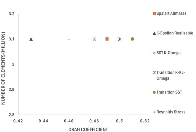
Table 15. CRF turbulence model test results.

Figure 28: CRF model 1: Turbulence test	Figure 29: CRF model 2: Turbulence test
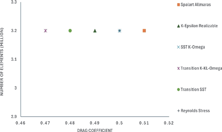
Figure 30: CRF model 3: Turbulence test

Figure 28. CRF model 1: Turbulence test.

Figure 29. CRF model 2: Turbulence test.

The 30° slant angle model resulted in a higher C_D value compared to the other models, but for varying air speeds, the drag value was almost constant. An optimal angle for the square back maintains the airflow attached to the surface.

A smaller wake region was observed in this case (refer to Table 16). The overall drag value does not vary as the air speed increases. The 30° slant angle model proved to be an effective device for reducing the drag under high-speed conditions.

Table 16. Comparison of velocity contours of baseline and optimized models.

Baseline model
Optimised model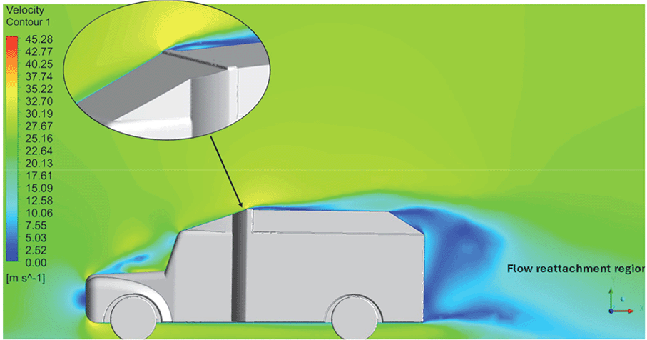

CRF model 2 exhibited the lowest overall drag when compared to the other models. The effective angle of the front wind deflector reduces drag accumulation in the frontal region of the truck. CRF Model 2 is the best wind deflector model for trucks. The optimal angle and height of the deflector resulted in smooth airflow above the truck.

4.5.5 Comparative analysis

Table 16 compares the velocity contours of the baseline and optimized models. A small wake region was observed in the optimized model. Flow attachment occurs quickly in the optimized model. The low air velocity regions (blue shaded regions) are more streamlined in the optimized model. Abrupt flow separation was observed in the baseline model.

Table 17 compares the velocity streamlines of the baseline and optimized models. The air flow recirculation regions were reduced in the optimized model. The gap enclosure directs the airflow smoothly around the truck. A large vortex formation was observed in both cases.

Table 17. Comparison of velocity streamlines of baseline and optimized models.

Baseline model
Optimised model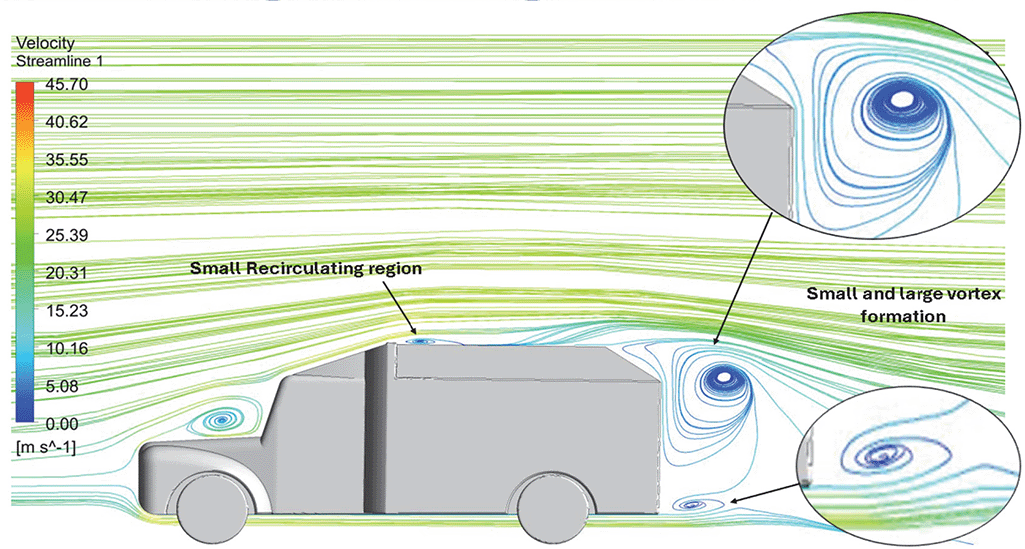

small-scale vortex formations are minimized in the optimized model, thereby improving the air flow around the truck model.

Table 18 compares the surface pressures of the baseline and optimized models. The Trailer body surface pressure was minimized in the optimized model. The pressure ranges from -525 Pa to 146 Pa. The frontal area experienced the highest pressure per unit area. The CRF and gap enclosures were effective in minimizing the surface pressure near the trailer body.

Table 18. Table of comparison for surface pressure of baseline and optimized models.

Baseline model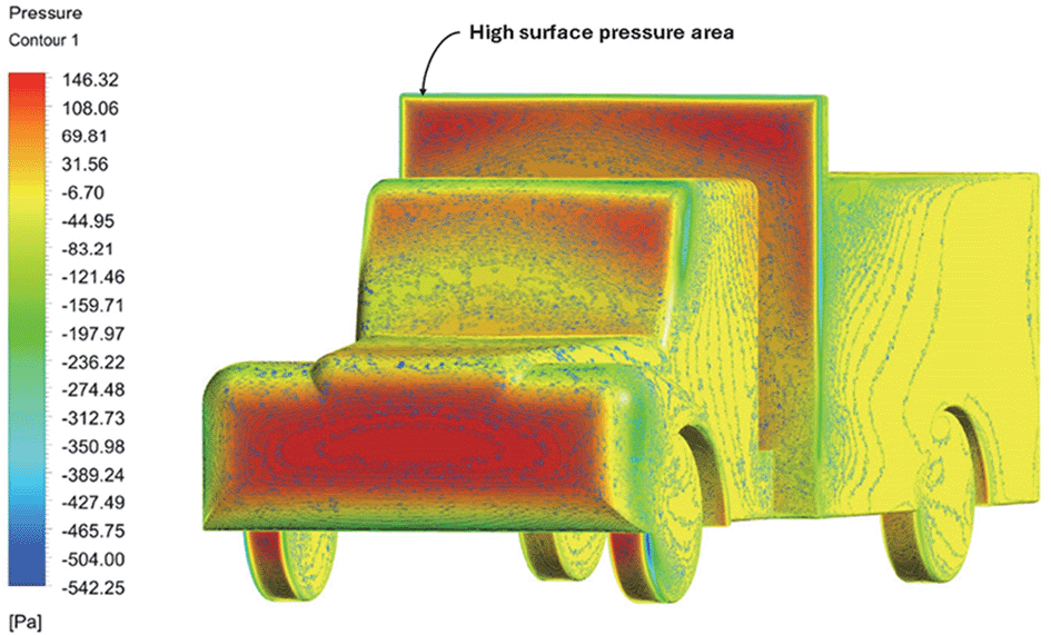
Optimised model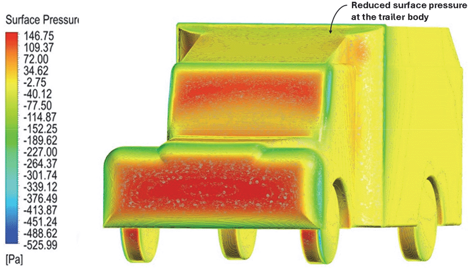

Table 19 shows the changes in different drag coefficient values. Effective design optimization results in a significant decrease in the drag of the truck geometry. An overall drag value of C_D = 0.45 for the optimised model is achieved for varying velocity conditions. The maximum drag reduction is achieved at 90 km/h. At higher speeds, the drag value was minimal for the optimized truck when compared to the baseline model.

Table 19. Comparison of baseline and optimized models.

Velocity (Kmph)	Baseline model	Optimised model	% Drag reduction
40	0.49	0.40	18.3
50	0.50	0.42	16.0
60	0.68	0.45	33.8
70	0.72	0.47	34.7
80	0.92	0.49	46.7
90	1.20	0.51	57.5

A significant drag reduction was obtained from the optimized model analysis. The flow modifications at the rear of the truck are observed owing to the effective slant angle of the square-back. The gap enclosure successfully eliminated flow recirculation in the truck-trailer gap region. This study successfully reduced the overall drag of the baseline truck using various design optimizations and effective turbulence models using a numerical method. Under high-speed conditions, the truck’s overall drag value was reduced in the case of the optimized model ( Figures 30 and 31)

Figure 30. CRF model 3: Turbulence test.

Figure 31. Varying velocity vs C_D for slant angle models.

Figure 32. Varying velocity vs C_D for CRF models.

.

The optimized model resulted in an effective 18% drag reduction when compared to the baseline model for an economy speed of 40 km/h. As shown in Figure 33, the overall drag coefficient value for the optimized model was much lower than that of the baseline model.

Figure 33. Comparison graph of C_D for baseline and optimised model.

In Figure 34, we can observe that the grid and turbulence tests have moderate drag values, and the final optimized model performs better than the baseline and reference paper models, indicating improvements in overall aerodynamics.

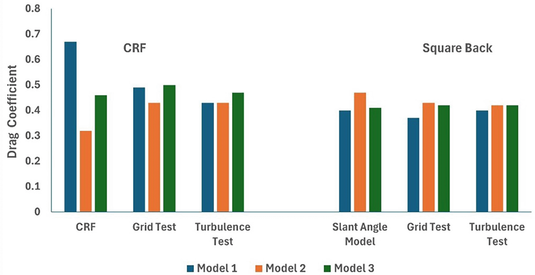
Figure 34. Drag values of various parameters for CRF and square back models.

Figure 35 shows a comparison of the drag coefficients of the different models. The baseline model had the highest drag, while the optimized model, best CRF model, and best slant angle model showed significant reductions, indicating improved aerodynamic efficiency.

Figure 35. Best of the comparative drag coefficient values.

In Table 20, the C_D values of all models for different parameters are given. Lower drag coefficient values

Table 20. Drag coefficient values of various parameters.

	Drag Coefficient (C_D)
	Model 1	Model 2	Model 3
CRF Model	0.67	0.32	0.46
Grid Test	0.49	0.43	0.5
Turbulence Test	0.43	0.43	0.47

	Model 1	Model 2	Model 3
Slant Angle Model	0.4	0.47	0.41
Grid Test	0.37	0.43	0.42
Turbulence Test	0.4	0.42	0.42

.

5. Conclusions and future works

The objective of this study was to investigate the airflow behavior around a truck. In this study, a cab-roof fairing for effective drag reduction is proposed. A numerical analysis was performed for the baseline truck model, and the results obtained were compared and validated with reference papers. The least computational error for the baseline analysis was 2.8%. Passive drag reduction devices, such as cab roof fairing, proved to be an effective method for improving the overall aerodynamic efficiency of trucks by reducing drag.

The obtained drag coefficient value of the simulation was accurate and closer to the experimental reference value. Different turbulence models were tested, and the K-epsilon turbulence model, both standard and realizable, resulted in accurate results and a minimum computational error of 4%. The K-epsilon turbulence model proved to be very effective for free-flow conditions by providing a faster solution convergence.

Various CRF models and slant angle modifications were employed to optimize the truck. Two of the best models out of the nine design optimizations were chosen for the final simulation. Various grid tests were conducted to determine the optimal mesh for the simulations. The gap enclosures remarkably reduced the streamwise vorticity in the gap region between the truck cabin and the trailer. The wind deflector achieved optimal results by smoothly directing the airflow. The fairings delayed the flow separation on the side surfaces and blocked any inward flow into the gaps, thereby effectively reducing the drag. These modifications were effective in reducing the drag of the truck model.

The optimized model results showed a significant drag reduction at higher speeds. A drag reduction of 18 % %was achieved for the optimized model through effective CRF installation. The flow contours were analyzed and compared with the baseline model results. The optimized slant angle model results showed a reduced wake region size at the rear with an improved airflow structure around the truck cabin. The velocity streamline plot shows smooth flow lines above the optimized truck cabin.

Enhancing the aerodynamic features of the entire vehicle is essential. Various components, such as side skirts, underbody coverings, and gap extenders, are currently underutilized in commercial vehicles. Enhancements to the gap enclosure are required because a complete enclosure will obstruct the side air intake vent in the SCV and LCV. Hence, it is necessary to optimize the shape and geometry of aerodynamic devices to reduce drag and improve aerodynamic efficiency.

Ethics and consent

Ethics and consent were not required.

Data availability

All underlying data are available in the article itself.

References

1. Hariram A, Koch T, Mårdberg B, et al.: A study in options to improve aerodynamic profile of heavy-duty vehicles in Europe. Sustainability (Switzerland). Oct. 2019; 11(19). Publisher Full Text
2. Bello-Millán FJ, Mäkelä T, Parras L, et al.: Experimental study on Ahmed’s body drag coefficient for different yaw angles. J. Wind Eng. Ind. Aerodyn. Oct. 2016; 157: 140–144. Publisher Full Text
3. Kücüksariyildiz H, Canli E, Carman K: Experimentally detected aerodynamic drag coefficient of the agricultural tractor form considering effects of windshield angle and hood front shape. Energy. Jun. 2024; 296: 131167. Publisher Full Text
4. Irving Brown YA, Windsor S, Gaylard AP: The effect of base bleed and rear cavities on the drag of an SUV. SAE Technical Papers. SAE International; 2010. Publisher Full Text
5. Garcia De La Cruz JM, Brackston RD, Morrison JF: Adaptive Base-Flaps under Variable Cross-Wind. SAE Technical Papers. SAE International; Aug. 2017. Publisher Full Text
6. Shankar G, Devaradjane G: Experimental and computational analysis on aerodynamic behavior of a car model with vortex generators at different yaw angles. J. Appl. Fluid Mech. 2018; 11(1): 285–295. Publisher Full Text
7. Kim JJ, Hong J, Lee SJ: Bio-inspired cab-roof fairing of heavy vehicles for enhancing drag reduction and driving stability. Int. J. Mech. Sci. Oct. 2017; 131-132: 868–879. Publisher Full Text
8. Kim JJ, Kim J, Lee SJ: Substantial drag reduction of a tractor-trailer vehicle using gap fairings. J. Wind Eng. Ind. Aerodyn. Dec. 2017; 171: 93–100. Publisher Full Text
9. Kim JJ, Kim J, Hann T, et al.: Considerable drag reduction and fuel saving of a tractor–trailer using additive aerodynamic devices. J. Wind Eng. Ind. Aerodyn. Aug. 2019; 191: 54–62. Publisher Full Text
10. Martín-Alcántara A, Sanmiguel-Rojas E, Gutiérrez-Montes C, et al.: Drag reduction induced by the addition of a multi-cavity at the base of a bluff body. J. Fluids Struct. 2014; 48: 347–361. Publisher Full Text
11. Ralin Bukreev K: Shape optimisation of teardrop trailers to minimise aerodynamic drag in articulated lorries. Int. J. Thermofluids. May 2023; 18: 100334. Publisher Full Text
12. Delassaux F, Mortazavi I, Herbert V, et al.: Numerical analysis of unsteady flow features around a realistic Estate vehicle with hybrid RANS/LES methods. Comput. Fluids. Aug. 2023; 262: 105935. Publisher Full Text
13. Goc KA, Lehmkuhl O, Park GI, et al.: Large eddy simulation of aircraft at affordable cost: a milestone in computational fluid dynamics. Flow. Dec. 2021; 1. Publisher Full Text
14. Abdellah E, Wang B: CFD analysis on effect of front windshield angle on aerodynamic drag. IOP Conference Series: Materials Science and Engineering. Institute of Physics Publishing; Sep. 2017. Publisher Full Text
15. Qin P, Ricci A, Blocken B: CFD simulation of aerodynamic forces on the DrivAer car model: Impact of computational parameters. J. Wind Eng. Ind. Aerodyn. May 2024; 248: 105711. Publisher Full Text
16. Aultman M, Wang Z, Auza-Gutierrez R, et al.: Evaluation of CFD methodologies for prediction of flows around simplified and complex automotive models. Comput. Fluids. Mar. 2022; 236: 105297. Publisher Full Text
17. Bedford J Truck Manual. http
18. Chowdhury H, Juwono R, Zaid M, et al.: An experimental study on of the effect of various deflectors used for light trucks in Indian subcontinent. Energy Procedia. Elsevier Ltd; 2019; pp. 34–39. Publisher Full Text
19. Datta B, Goel V, Garg S, et al.: Study of Various Passive Drag Reduction Techniques on External Vehicle Aerodynamics Performance: CFD Based Approach. International Research Journal of Engineering and Technology. 2008; p. 1851. Reference Source
20. Szodrai F: Quantitative analysis of drag reduction methods for blunt shaped automobiles. MDPI AG; Jun. 01, 2020. Publisher Full Text
21. Choi H, Lee J, Park H: Aerodynamics of heavy vehicles. Annu. Rev. Fluid Mech. Jan. 2014; 46: 441–468. Publisher Full Text

Comments on this article Comments (0)

Version 1

VERSION 1 PUBLISHED 26 Aug 2025

Author details Author details

¹ Department of Aeronautical & Automobile Engineering, Manipal Institute of Technology (MIT), Manipal Academy of Higher Education (MAHE), Manipal, Udupi, Karnataka, 576104, India
² Department of Mechanical & Industrial Engineering, Manipal Institute of Technology (MIT), Manipal Academy of Higher Education (MAHE), Manipal, Udupi, Karnataka, 576104, India

Madhav S Prabhu
Roles: Conceptualization, Data Curation, Formal Analysis

Sudheendra Prabhu K
Roles: Funding Acquisition, Investigation, Methodology, Resources

Amar A Murthy
Roles: Investigation, Software, Writing – Original Draft Preparation

Srinivas G
Roles: Investigation, Methodology, Project Administration, Supervision, Writing – Review & Editing

Competing interests

No competing interests were disclosed.

Grant information

The author(s) declared that no grants were involved in supporting this work.

Article Versions (1)

version 1

Published: 26 Aug 2025, 14:821

https://doi.org/10.12688/f1000research.163917.1

Copyright

© 2025 Prabhu MS et al. This is an open access article distributed under the terms of the Creative Commons Attribution License, which permits unrestricted use, distribution, and reproduction in any medium, provided the original work is properly cited.

Download

Export To

metrics

	Views	Downloads
F1000Research	-	-
PubMed Central Data from PMC are received and updated monthly.	-	-

Citations

0

SEE MORE DETAILS

CITE

how to cite this article

Prabhu MS, Prabhu K S, Murthy AA and G S. Aerodynamic Drag Reduction in Commercial Vehicle Using CFD-Based Design Optimisation [version 1; peer review: awaiting peer review]. F1000Research 2025, 14:821 (https://doi.org/10.12688/f1000research.163917.1)

NOTE: If applicable, it is important to ensure the information in square brackets after the title is included in all citations of this article.

track

receive updates on this article

Track an article to receive email alerts on any updates to this article.

Open Peer Review

Comments on this article Comments (0)

Version 1

VERSION 1 PUBLISHED 26 Aug 2025

Open Peer Review

Reviewer Status

AWAITING PEER REVIEW

Comments on this article

All Comments(0)

Add a comment

Sign up for content alerts

Browse by related subjects

[1] 1. Hariram A, Koch T, Mårdberg B, et al.: A study in options to improve aerodynamic profile of heavy-duty vehicles in Europe. Sustainability (Switzerland). Oct. 2019; 11(19). Publisher Full Text

[2] 2. Bello-Millán FJ, Mäkelä T, Parras L, et al.: Experimental study on Ahmed’s body drag coefficient for different yaw angles. J. Wind Eng. Ind. Aerodyn. Oct. 2016; 157: 140–144. Publisher Full Text

[3] 3. Kücüksariyildiz H, Canli E, Carman K: Experimentally detected aerodynamic drag coefficient of the agricultural tractor form considering effects of windshield angle and hood front shape. Energy. Jun. 2024; 296: 131167. Publisher Full Text

[4] 4. Irving Brown YA, Windsor S, Gaylard AP: The effect of base bleed and rear cavities on the drag of an SUV. SAE Technical Papers. SAE International; 2010. Publisher Full Text

[5] 5. Garcia De La Cruz JM, Brackston RD, Morrison JF: Adaptive Base-Flaps under Variable Cross-Wind. SAE Technical Papers. SAE International; Aug. 2017. Publisher Full Text

[6] 6. Shankar G, Devaradjane G: Experimental and computational analysis on aerodynamic behavior of a car model with vortex generators at different yaw angles. J. Appl. Fluid Mech. 2018; 11(1): 285–295. Publisher Full Text

[7] 7. Kim JJ, Hong J, Lee SJ: Bio-inspired cab-roof fairing of heavy vehicles for enhancing drag reduction and driving stability. Int. J. Mech. Sci. Oct. 2017; 131-132: 868–879. Publisher Full Text

[8] 8. Kim JJ, Kim J, Lee SJ: Substantial drag reduction of a tractor-trailer vehicle using gap fairings. J. Wind Eng. Ind. Aerodyn. Dec. 2017; 171: 93–100. Publisher Full Text

[9] 9. Kim JJ, Kim J, Hann T, et al.: Considerable drag reduction and fuel saving of a tractor–trailer using additive aerodynamic devices. J. Wind Eng. Ind. Aerodyn. Aug. 2019; 191: 54–62. Publisher Full Text

[10] 10. Martín-Alcántara A, Sanmiguel-Rojas E, Gutiérrez-Montes C, et al.: Drag reduction induced by the addition of a multi-cavity at the base of a bluff body. J. Fluids Struct. 2014; 48: 347–361. Publisher Full Text

[11] 11. Ralin Bukreev K: Shape optimisation of teardrop trailers to minimise aerodynamic drag in articulated lorries. Int. J. Thermofluids. May 2023; 18: 100334. Publisher Full Text

[12] 12. Delassaux F, Mortazavi I, Herbert V, et al.: Numerical analysis of unsteady flow features around a realistic Estate vehicle with hybrid RANS/LES methods. Comput. Fluids. Aug. 2023; 262: 105935. Publisher Full Text

[13] 13. Goc KA, Lehmkuhl O, Park GI, et al.: Large eddy simulation of aircraft at affordable cost: a milestone in computational fluid dynamics. Flow. Dec. 2021; 1. Publisher Full Text

[14] 14. Abdellah E, Wang B: CFD analysis on effect of front windshield angle on aerodynamic drag. IOP Conference Series: Materials Science and Engineering. Institute of Physics Publishing; Sep. 2017. Publisher Full Text

[15] 15. Qin P, Ricci A, Blocken B: CFD simulation of aerodynamic forces on the DrivAer car model: Impact of computational parameters. J. Wind Eng. Ind. Aerodyn. May 2024; 248: 105711. Publisher Full Text

[16] 16. Aultman M, Wang Z, Auza-Gutierrez R, et al.: Evaluation of CFD methodologies for prediction of flows around simplified and complex automotive models. Comput. Fluids. Mar. 2022; 236: 105297. Publisher Full Text

[17] 17. Bedford J Truck Manual. http

[18] 18. Chowdhury H, Juwono R, Zaid M, et al.: An experimental study on of the effect of various deflectors used for light trucks in Indian subcontinent. Energy Procedia. Elsevier Ltd; 2019; pp. 34–39. Publisher Full Text

[19] 19. Datta B, Goel V, Garg S, et al.: Study of Various Passive Drag Reduction Techniques on External Vehicle Aerodynamics Performance: CFD Based Approach. International Research Journal of Engineering and Technology. 2008; p. 1851. Reference Source

[20] 20. Szodrai F: Quantitative analysis of drag reduction methods for blunt shaped automobiles. MDPI AG; Jun. 01, 2020. Publisher Full Text

[21] 21. Choi H, Lee J, Park H: Aerodynamics of heavy vehicles. Annu. Rev. Fluid Mech. Jan. 2014; 46: 441–468. Publisher Full Text

Aerodynamic Drag Reduction in Commercial Vehicle Using CFD-Based Design Optimisation

Abstract

Background

Method

Results

Conclusions

Keywords

1. Introduction

Figure 1. Various aerodynamic devices installed on a heavy commercial vehicle.1

2. Literature review

2.1 Research gaps

2.2 Research objectives

3. Methodology

Figure 2. Methodology flowchart.

3.1 Baseline analysis

Table 1. Truck model dimensions (1/10th scale).17

Figure 3. Bedford truck 3D model (Side view).

Figure 4. Bedford truck 3D model (Front view).

Figure 5. Blueprint of the Bedford J series truck.17

Table 2. Mesh details for the truck and enclosure.

Figure 6. Mesh generated for the enclosure and the truck surface.

Figure 7. Computational fluid domain dimensions and boundary conditions.

Table 3. Boundary conditions for the named selections.

Figure 8. Turbulence model settings and solution methods.

Table 4. Results of grid independence test.

Figure 9. Reference values.

(1)

(2)

(3)

(4)

(5)

(6)

Figure 10. Drag coefficient plot for baseline model.

4. Results and discussions

4.1 Grid independence test

Figure 11. Number of elements vs drag coefficient for baseline model.

4.2 Varying turbulence models

Figure 12. Turbulence model performance vs CD for the best grid size.

Table 5. Turbulence model comparison results.

Table 6. Comparison of velocity contour and streamline contour of reference paper result with different viscous model results.18

Table 7. Comparison of velocity contour and streamline contour of reference paper result with different viscous model results.18

Table 8. Comparison of velocity contour and streamline contour of reference paper result with different viscous model results.18

Table 9. Comparison of velocity contours.

Table 10. Comparison of velocity streamlines.

Figure 13. K-Epsilon model velocity contour.

Figure 14. Reynolds stress model velocity contour.

Figure 15. K-Epsilon model velocity streamline.

Figure 16. Reynolds stress model velocity streamline.

4.3 Varying inlet velocity

Table 11. Values of drag coefficient for different air velocity.

Figure 17. Varying velocity vs drag coefficient for baseline truck model.

Figure 18. Velocity contour and velocity streamline at 40 Kmph.

Figure 19. Velocity contour and velocity streamline at 90 Kmph.

4.4 Baseline model comparison and validation

Figure 20. Drag coefficient (CD) as a function of wind speed.18

Figure 21. Drag coefficient (CD) vs varying velocity, comparison of reference paper18 model and present work baseline truck model results.

4.5 Optimised model analysis

Figure 22. Various CRF and square back design modifications for the baseline truck.

Figure 23. Optimised truck model (Isometric view).

Figure 24. Optimised truck model (Side view).

Table 12. CRF model dimensions.

Table 13. Gap fairing dimensions (1/10th scale).

Table 14. Square back modification dimensions (1/10th scale).

Figure 25. CRF attached with truck cabin and gap enclosure.

Figure 26. Square back geometry (Side view).

Figure 27. Simplified three-dimensional square back Ahmed model.21

Table 15. CRF turbulence model test results.

Figure 28. CRF model 1: Turbulence test.

Figure 29. CRF model 2: Turbulence test.

Table 16. Comparison of velocity contours of baseline and optimized models.

Table 17. Comparison of velocity streamlines of baseline and optimized models.

Table 18. Table of comparison for surface pressure of baseline and optimized models.

Table 19. Comparison of baseline and optimized models.

Figure 30. CRF model 3: Turbulence test.

Figure 31. Varying velocity vs CD for slant angle models.

Figure 32. Varying velocity vs CD for CRF models.

Figure 33. Comparison graph of CD for baseline and optimised model.

Figure 34. Drag values of various parameters for CRF and square back models.

Figure 35. Best of the comparative drag coefficient values.

Table 20. Drag coefficient values of various parameters.

Figure 1. Various aerodynamic devices installed on a heavy commercial vehicle.¹

Table 1. Truck model dimensions (1/10^th scale).¹⁷

Figure 5. Blueprint of the Bedford J series truck.¹⁷

Figure 12. Turbulence model performance vs C_D for the best grid size.

Table 6. Comparison of velocity contour and streamline contour of reference paper result with different viscous model results.¹⁸

Table 7. Comparison of velocity contour and streamline contour of reference paper result with different viscous model results.¹⁸

Table 8. Comparison of velocity contour and streamline contour of reference paper result with different viscous model results.¹⁸

Figure 20. Drag coefficient (C_D) as a function of wind speed.¹⁸

Figure 21. Drag coefficient (C_D) vs varying velocity, comparison of reference paper¹⁸ model and present work baseline truck model results.

Table 13. Gap fairing dimensions (1/10^th scale).

Table 14. Square back modification dimensions (1/10^th scale).

Figure 27. Simplified three-dimensional square back Ahmed model.²¹

Figure 31. Varying velocity vs C_D for slant angle models.

Figure 32. Varying velocity vs C_D for CRF models.

Figure 33. Comparison graph of C_D for baseline and optimised model.