CBN2Path: an R/Bioconductor package for the analysis of cancer progression pathways using Conjunctive Bayesian Networks

Implementation

CBN2Path is implemented as a standard R package and hosted in the Bioconductor repository. Furthermore, the developed version of CBN2Path is available on GitHub. All functions were documented, and examples were included. The main functions included in CBN2Path are listed in Table 1, and their features and capabilities are described in detail in the tutorial (vignette) accompanied by the package. CBN2Path can be installed and used mainly on Unix platforms.

if (!require("BiocManager", quietly = TRUE))
   install.packages("BiocManager")
BiocManager::install("CBN2Path")

During the installation of CBN2Path, other packages that it depends on are automatically installed, including coda, cowplot, doMC, foreach, ggplot2, ggraph, grDevices, graphics, igraph, magrittr, patchwork, rlang, R6, stats, and tidygraph.

Operation

CBN2Path provides a unifying interface to implement different CBN models, which are utilized to facilitate the quantification, visualization, and analysis of mutational pathways. The CBN2Path has three main functionalities.

Figure 1. Workflow I.

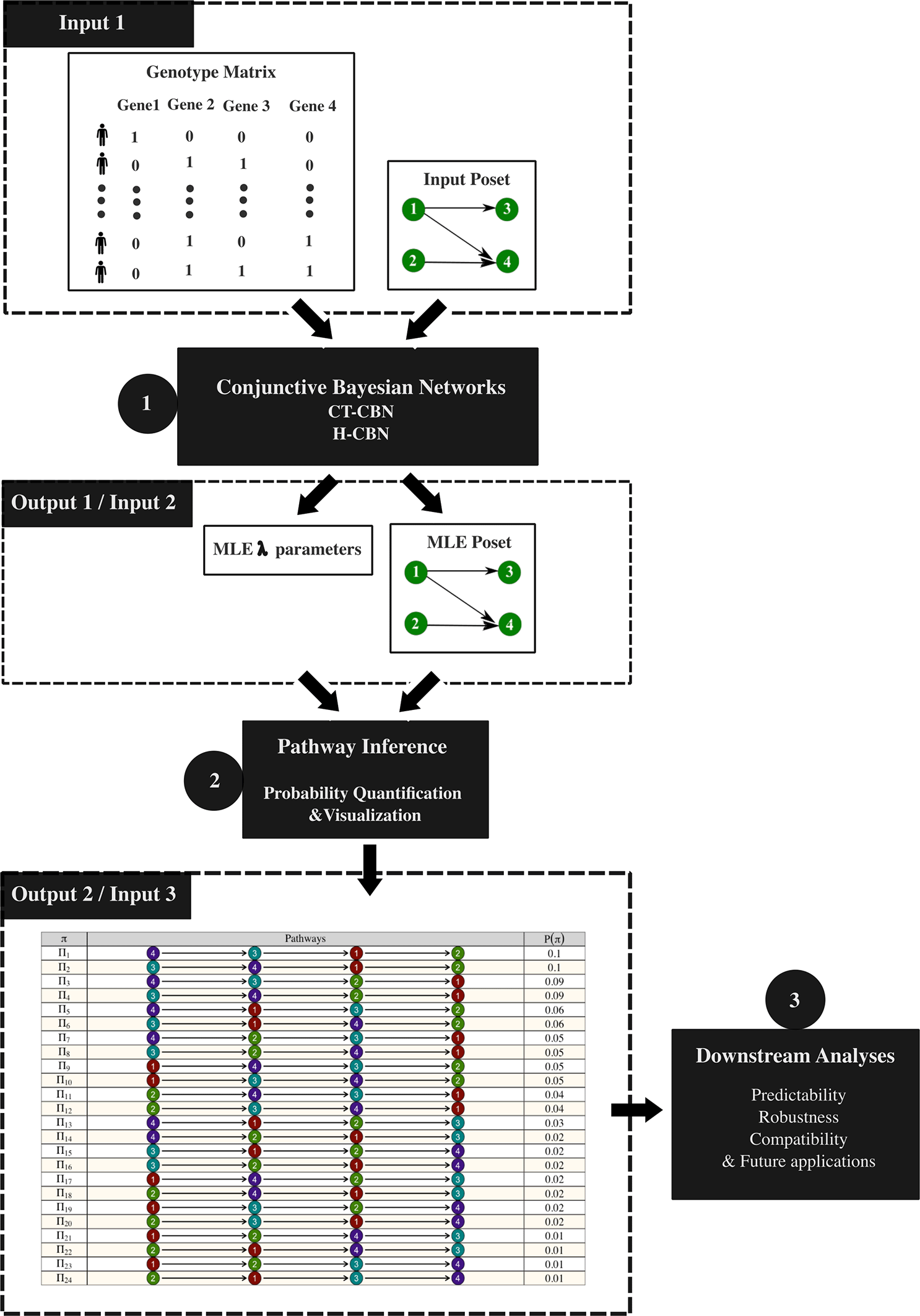
CBN models (CT-CBN or H-CBN) take the genotype matrix and a given poset as input, and then output the estimated λ vector and the MLE poset (step 1), which will be used by the pathway inference functions to produce the inferred pathway probability distribution (step 2) that will be subsequently used by other downstream functions to measure different properties of the pathway probabilities (step 3).

Figure 2. Workflow II.

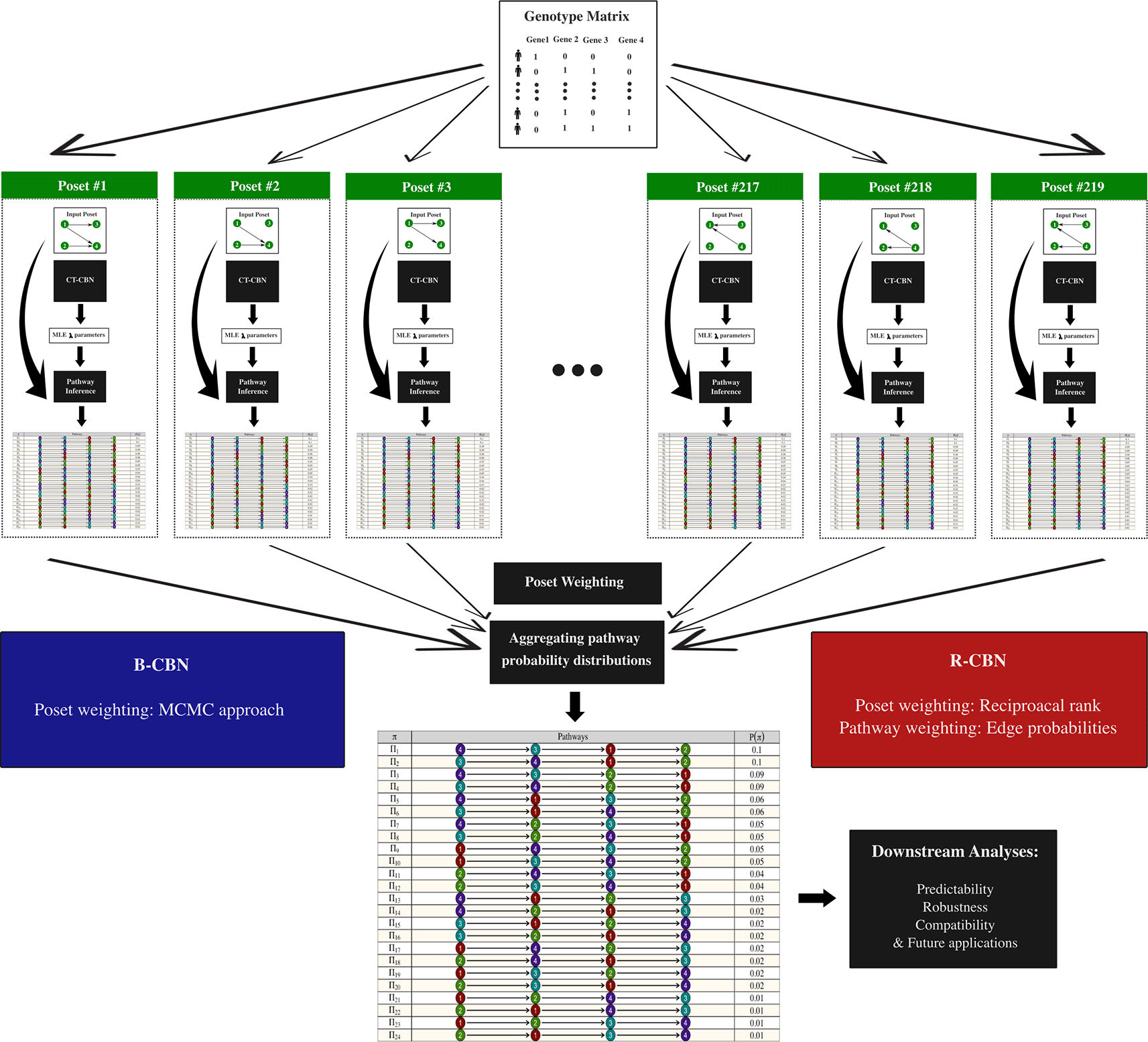
The R-CBN and B-CBN approaches require an alternative workflow for quantifying the pathway probability distributions, which only takes a genotype matrix as the input. Basically, under all 219 potential posets, the λ parameters are estimated using CT-CBN. Consequently, 219 different probability distributions are derived, which are then aggregated to generate the ultimate pathway probability distribution that will be used by the downstream functions for further analyses. Note that the B-CBN method utilizes an MCMC approach for weighting the posets, which is needed in the aggregation step.⁴ In contrast, in the R-CBN method, the likelihood outputted from the CT-CBN model under each of the 219 posets are considered, and pathways are weighted based on their reciprocal rank in terms of likelihood. Furthermore, R-CBN weights the pathways and updates their probabilities using their corresponding edge (marginal) probabilities.⁵ Note that in the workflow II there is no sequential input-output arrangement, but rather we have one single input (the genotype matrix) and one single output (the ultimate probability distribution). In other words, the intermediate functions are called internally, without a direct interface with the user.

Figure 3. Analysis and visualization of fitness landscapes.

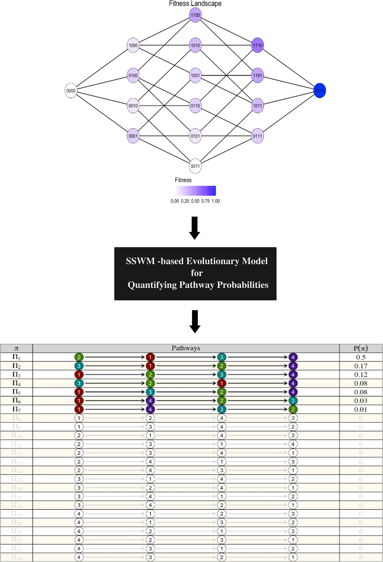
CBN2Path enables visualization of fitness landscapes and quantifying pathway probability distributions based on evolutionary models under the Strong-Selection Weak-Mutation (SSWM) assumption.⁷

Workflow I: CT-CBN and H-CBN based quantification of pathway probabilities

Preparing the input data

As shown in Figure 2, the original implementation of the CT-CBN and H-CBN models requires two input files: i) a “.pat” file, which contains binary genotype data, and ii) a “.poset” file that encodes a given poset. CBN2Path avoids reading files but accepts two matrices that are obtained after reading the above files. Importantly, to store input posets and genotype matrices, CBN2Path implements its own data structure, Spock, which includes read_pattern and read_poset methods to read, respectively the “.pat” and “.poset” files in the spock-data type.

library(CBN2Path)
example_path <- getExamples()[1]
input_poset <- readPoset(example_path)
input_pattern <- readPattern(example_path)
input_1 <- Spock$new(
     poset = input_poset$sets,
     numMutations = input_poset$mutations,
     genotypeMatrix = input_pattern
)

Alternatively, input matrices can be created directly without reading from a file. For example:

# The poset
dag <- matrix(c(3, 3, 4, 4, 1, 2, 1, 2), 4, 2)

# The genotype matrix
set.seed(100)

gen_1<-c(rep(0,150),sample(c(0,1),25,replace=TRUE),rep(0,25))
gen_2<-c(rep(0,175),sample(c(0,1),25,replace=TRUE))
gen_3<-c(rep(0,50),sample(c(0,1),100,replace=TRUE),rep(1,50))
gen_4<-c(sample(c(0,1),100,replace=TRUE),rep(0,50),rep(1, 50))
g_mat<-matrix(c(gen_1, gen_2, gen_3, gen_4), 200, 4)
g_mat<-cbind(1, g_mat)

# Preparing input of the ct-cbn/h-cbn methods
input_2 <- Spock$new(
     poset = dag,
     numMutations = 4, genotypeMatrix = g_mat
)

Note that the first column of the genotype matrix must always be one, whereas each of the other columns corresponds to a given mutational event. Therefore, the number of columns in the genotype matrix must be equal to the number of mutations considered plus one.

In the second example, the genotypes are generated such that the mutation orders never violate the restrictions in the temporal ordering between mutations imposed by the corresponding poset. For example, mutations 1 and 2 occur when mutations 3 and 4 have already occurred. To allow violation of the restrictions, one can use the genotypeMatrixMutator function to add false positives and false negatives of a given rate. In the following example, the g_mat matrix is converted to the g_mat_mut matrix by adding false positive and false negative rates of 0.3 and 0.2, respectively:

temp <- g_mat[,2:5]
temp_mut <- genotypeMatrixMutator(temp, 0.3, 0.2)
g_mat_mut <- cbind(1, temp_mut)
# Preparing input of the ct-cbn/h-cbn methods
input_3 <- Spock$new(
     poset = dag,
     numMutations = 4,
     genotypeMatrix = g_mat_mut
)

Note that the first column of the genotype matrix must always remain one. Therefore, we did not pass the first column to genotypeMatrixMutator function.

Running the CBN models

Having prepared the input files, it is now easy to run the CBN models using ctcbnSingle and hcbnSingle.

# CT-CBN
results_c1 <- ctcbnSingle(input_1)
results_c2 <- ctcbnSingle(input_2)
results_c3 <- ctcbnSingle(input_3)
# H-CBN
results_h1 <- hcbnSingle(input_1)
results_h2 <- hcbnSingle(input_2)
results_h3 <- hcbnSingle(input_3)

Below, we can see how to obtain the estimated λ values and the corresponding likelihood for the first example.

# The estimated lambda values
ml_lambda_c1 <- results_c1[[1]]$lambda

# The likelihood
loglikelihood_c1 <- results_c1[[1]]$summary[4]

Furthermore, the maximum-likelihood poset can be identified and visualized using visualizeCBNModel function.

# The MLE poset
ml_poset_c1 <-results_c1[[1]]$poset$sets
# visualizing the MLE
visualizeCBNModel(ml_poset_c1)

It is important to mention that we have an alternative implementation of the CBN models, namely the ctcbn and hcbn functions, which accept a list of posets as input and accordingly produce a list of λ vectors, a list of likelihood values, and a list of MLE posets. This strategy is utilized in the second workflow, which is specifically suited for analyzing mutational quartets and pathways of length four.

# The collection of all 219 potential posets
posets <- readRDS(system.file("extdata", "Posets.rds", package = "CBN2Path")) #
Input preparation
input_4 <- Spock$new(
     poset = posets,
     numMutations = 4,
     genotypeMatrix = g_mat
)
# Running the ctcbn function
results_c4 <- ctcbn(input_4)
# Running the hcbn function
results_h4 <- hcbn(input_4)

Note that the collection of all 219 potential posets for analyzing mutational quartets is already accessible within the package, which is read and stored in the first line of the above code.

Inferring pathway probability distributions

The output of the CBN models, namely the estimated λ values and the MLE poset, can be used as the input of the pathProbCBN function, which quantifies the pathway probability distribution (P(Π)). In the example below, the results of the second example obtained in the previous section (results_c2 and results_h2) are used.

# The first input: The MLE poset (the output of the CBN models)
dag_c2 <- results_c2[[1]]$poset$sets
dag_h2 <- results_h2[[1]]$poset$sets

#The second input: The estimated Lambda values (the output of the CBN models)
lambda_c2 <- as.numeric(results_c2[[1]]$lambda)
lambda_h2 <- as.numeric(results_h2[[1]]$lambda)
# Quantifying the pathway probability distributions
prob_c2 <- pathProbCBN(dag_c2, lambda_c2, 4)
prob_h2 <- pathProbCBN(dag_h2, lambda_h2, 4)

In this example, prob_c2 and prob_h2 are vectors of length 24, each representing one of the 24 pathways.

Downstream analyses

The quantified pathway probability distributions are used as the input of other functions used in the downstream steps for visualization (visualizeProbabilities) and quantification of the predictability (predictability), or measuring the divergence between probability distributions (jensenShannonDivergence):

# Visualization of pathways and their probabilities
visualizeProbabilities(prob_c2)
visualizeProbabilities(prob_h2)
# Quantification of predictability score for a given probability distribution
pred_c2 <- predictability(prob_c2, 4)
pred_h2 <- predictability(prob_h2, 4)
# Quantification of the Jensen-Shannon Divergence (JSD) between a pair of distributions
jsd <- jensenShannonDivergence(prob_c2, prob_h2)

Workflow II: B-CBN and R-CBN based inference of pathway probability distributions

The second workflow for quantifying pathway probabilities was designed specifically for implementing the R-CBN and B-CBN algorithms to enable the robust inference of pathway probability distributions. It is specifically suited for analyzing mutational quartets and pathways of length 4. The ctcbn function that takes the exhaustive list of 219 posets as input is an integral part of this workflow, which makes it easy to work with, as the user only needs to input a genotype matrix.

Running the R-CBN model

R-CBN weighs the 219 posets based on their reciprocal rank in terms of likelihood, and a second pathway-based weighting layer is employed. However, the user only needs to work directly with the pathProbQuartetRCBN function, because intermediate functions such as posetWeightingRCBN, pathwayWeightingRCBN, edgeMarginalized, pathEdgeMapper and pathNormalization are taken care of internally.

g_mat2 <- g_mat[,2:5]
prob_r2 <- pathProbQuartetRCBN(g_mat2)

Note that this function only needs a genotype matrix as the input and does not require the first column of the matrix to be one; therefore, we needed to remove the first column from the gMat matrix that we previously produced.

Running the B-CBN model

Although the B-CBN algorithm is fundamentally different from the R-CBN algorithm, particularly in terms of how the posets are weighted, which strongly affects the internal implementation of the intermediate functions, the user interface is exactly the same. The pathProbQuartetBCBN function is defined as

prob_b2 <- pathProbQuartetBCBN(g_mat2)

CBN2Path also provides a similar implementation for CT-CBN and H-CBN.

prob_c2 <- pathProbQuartetCTCBN(g_mat2)
prob_h2 <- pathProbQuartetHCBN(g_mat2)

Having determined the pathway probabilities, downstream analysis can be performed similarly to those in the first workflow. Furthermore, pathway compatibilities (c(Π)) can be measured directly from a genotype matrix, and their correlation with pathway probabilities (P(Π)) can be calculated as

pathway_c2 <- pathwayCompatibilityQuartet(g_mat2)
rho_c2 <- cor(pathway_c2, prob_c2, method = "spearman")

Analyzing fitness landscapes

CBN2Path also provides functions for the analysis and visualization of fitness landscapes. For example, after assigning a fitness vector f to the set of binary genotypes of length four, which can be enumerated by the generateMatrixGenotypes function, we can calculate the corresponding pathway probability distribution under the SSWM-based evolutionary model using the pathProbSSWM function as follows:

f <- c(0, 0.1, 0.2, 0.1, 0.2, 0.4, 0.3, 0.2, 0.2, 0.1, 0, 0.6, 0.4, 0.3, 0.2, 1)
g <- generateMatrixGenotypes(4)
Prob_w<-pathProbSSWM(f,4)

Furthermore, the fitness landscape can be visually inspected using the visualizeFitnessLandscape function, as follows:

visualizeFitnessLandscape(f)