Keywords
Machine learning, Digital soil mapping, Precision agriculture, Systematic review

This article is included in the Agriculture, Food and Nutrition gateway.
This article is included in the Artificial Intelligence and Machine Learning gateway.
Machine learning, Digital soil mapping, Precision agriculture, Systematic review
Soil health constitutes the foundation of agricultural productivity, food security, and ecosystem sustainability (Lal, 2015). Healthy soils support nutrient cycling, water filtration, carbon sequestration, and biodiversity, functions essential for both crop production and environmental quality (Lehmann et al., 2020). However, global soil degradation, including erosion, nutrient depletion, salinization, and organic matter decline, threatens agricultural systems worldwide, with annual economic losses estimated at USD 400 billion (FAO, 2022).
The paradigm shift from traditional soil survey to digital soil mapping (DSM) represents a transformative advance in soil science (McBratney et al., 2003; Minasny & McBratney, 2016). DSM leverages the “scorpan” framework, soil formation factors (climate, organisms, relief, parent material, age, and space) predicted using environmental covariates and statistical models (McBratney et al., 2003). Traditional soil mapping relied on expert knowledge and field observations, but the increasing availability of remote sensing data and computational power has enabled quantitative, data-driven approaches (Arrouays et al., 2014).
Precision agriculture, managing agricultural inputs site-specifically, demands high-resolution soil maps at field or sub-field scales (<100 Ha) (Gebbers & Adamchuk, 2010). Such maps inform variable-rate fertilization, liming, irrigation, and other management decisions, potentially reducing input costs while improving yields and environmental outcomes. The Agriculture 4.0 paradigm, characterized by digitalization and data-driven decision-making, has accelerated the adoption of advanced analytical tools for soil management (Latino et al., 2021). For smallholder farmers in tropical regions, field-scale soil health information is particularly critical given the spatial heterogeneity of tropical soils and limited access to conventional laboratory analysis (Vanlauwe et al., 2015). Recent studies on Indonesian soils have highlighted the influence of land-use type on soil properties, emphasizing the need for site-specific assessments (Sulaeman et al., 2025).
Machine learning (ML) has emerged as a powerful complement to traditional statistical and geostatistical approaches in soil science (Padarian et al., 2020). Several factors drive this adoption. First, ML algorithms can capture complex, non-linear relationships between soil properties and environmental covariates without requiring pre-specified functional forms (Hengl et al., 2017). Second, ML methods handle high-dimensional data effectively, integrating spectral bands, topographic indices, climatic variables, and categorical information (Wadoux et al., 2020). Third, ensemble approaches such as Random Forest (Breiman, 2001) and XGBoost (T. Chen & Guestrin, 2016) provide robust predictions with built-in feature importance and regularization.
The availability of open-access remote sensing data, Landsat (since 1972), Sentinel-2 (since 2015), and MODIS, has exponentially increased the data available for soil mapping (Rossel et al., 2016). Concurrently, advances in computational infrastructure (cloud computing, GPUs) have made complex ML implementations accessible to soil scientists. UAV-based platforms now provide ultra-high-resolution (cm-scale) imagery, enabling plot-level soil property estimation. Field-scale applications have been demonstrated in various contexts, including gully erosion mitigation in South Africa using ML-based DSM approaches (Du Plessis et al., 2020).
However, the application of ML in soil science is not without challenges. Spatial autocorrelation violates assumptions of independent observations in standard cross-validation, potentially leading to over-optimistic performance estimates. Model interpretability, understanding why ML models make certain predictions, remains limited, constraining trust and adoption by agronomists and farmers (Samek et al., 2020). Recent advances in explainable artificial intelligence (XAI) have begun to address these interpretability challenges. For instance, Rashad et al. (2024) demonstrated how explainable ML and causal analysis can reveal ecosystem service relationships across scales, providing a framework applicable to soil health mapping. Furthermore, geographic and climatic biases in published studies may limit the transferability of findings to understudied regions, particularly the tropics.
Despite the growing body of literature on ML applications for soil property prediction, several gaps persist. First, most systematic reviews have focused on continental or global scales (Hengl et al., 2017; Padarian et al., 2020) rather than field-scale applications directly relevant to farm management. Second, the relative performance of ensemble versus single classifiers in field-scale contexts remains insufficiently quantified. Third, the magnitude of improvement of ML over conventional geostatistical methods (Kriging, IDW, OLS) has not been systematically benchmarked across diverse soil properties. Fourth, methodological challenges, particularly spatial overfitting, ground-truth data availability, and model interpretability, have not been comprehensively synthesized with attention to tropical agricultural systems.
These gaps are especially salient for regions such as Indonesia and Southeast Asia, where soil heterogeneity is high, cloud cover limits optical remote sensing, and smallholder farmers require actionable soil health information. The influence of land-use type on soil features in Indonesia underscores the importance of localized mapping approaches (Sulaeman et al., 2025). The absence of systematic evidence on field-scale ML performance in such contexts hinders both research prioritization and operational adoption.
Based on the PICOC framework (Population, Intervention, Comparison, Outcome, Context), we formulated four research questions:
1) What machine learning algorithms and input data types (satellite imagery, climate data, or in-situ sensors) are most dominant in field-scale soil health mapping studies for the period 2016–2026?
2) How does the performance of ensemble learning approaches (Random Forest, XGBoost) compare with single classifiers (SVM, ANN) in predicting chemical soil indicators (C-organic, pH, and total nitrogen)?
3) How significant are the accuracy improvements offered by machine learning algorithms compared to conventional geostatistical methods (Kriging/IDW) and parametric regression (OLS) in field-scale agricultural contexts?
4) What are the major methodological challenges in applying data science to field-scale soil mapping, particularly regarding spatial overfitting, ground-truth data availability, and model interpretability (XAI) in tropical agricultural systems?
This review offers several contributions. Practically, it provides evidence-based guidance for selecting ML approaches and validation protocols for operational field-scale soil mapping. Policy-wise, it identifies investment priorities for soil health monitoring in underrepresented regions. Methodologically, it establishes best practices for spatial validation and model evaluation. Theoretically, it contributes a framework for understanding ML performance in tropical soil systems, a context often overlooked in global syntheses. The integration of explainable ML perspectives, as demonstrated in ecosystem service studies (Rashad et al., 2024), provides a foundation for developing interpretable soil mapping models that can be adopted by practitioners.
This review focuses on studies published between 2016–2026 to capture the rapid expansion of deep learning applications since Sentinel-2 data became available and XGBoost was introduced. The spatial scale is limited to field-scale (<100 Ha) agricultural lands, excluding national or continental mapping. Target variables are restricted to chemical soil indicators (SOC, SOM, pH, N, P, K, CEC, salinity) relevant to soil health. Only supervised ML algorithms (RF, SVM, XGBoost, ANN, CNN, LSTM) are included; geostatistics-only studies and unsupervised methods are excluded. Studies must report at least one quantitative performance metric (R2, RMSE, MAE, CCC, or Kappa). The geographic scope is global but emphasizes studies in tropical or Southeast Asian contexts where available. The review also considers the applicability of Agriculture 4.0 frameworks (Latino et al., 2021) for translating ML-based soil maps into practical farming decisions.
This study employed a systematic literature review (SLR) design following the Preferred Reporting Items for Systematic Reviews and Meta-Analyses (PRISMA) 2020 guidelines (Page et al., 2021). The review protocol was developed a priori and documented internally. The review was not registered in PROSPERO as the protocol pertains to a methodological review without health-related outcomes. The PRISMA 2020 checklist was completed to ensure reporting transparency.
Eligibility criteria were defined based on the PICOC framework and operationalized for consistent application. Two reviewers independently applied the criteria; disagreements were resolved through discussion and consensus. Table 1 presents the complete inclusion and exclusion criteria.
We systematically searched six electronic databases: Scopus, Springer, ScienceDirect, Nature, IEEE Xplore, and Wiley. The search was conducted between January and March 2026, covering publications from January 2016 through March 2026. Hand-searching of reference lists supplemented the database searches.
The search strategy combined four thematic blocks using Boolean operators. The primary search string for Scopus (TITLE-ABS-KEY) was:
Block 1 (Machine Learning): (“machine learning” OR “random forest” OR “support vector machine” OR “svm” OR “xgboost” OR “gradient boosting” OR “artificial neural network” OR “ann” OR “deep learning” OR “cnn” OR “convolutional neural network” OR “ensemble learning” OR “data science”).
Block 2 (Soil Health): (“soil health” OR “soil quality” OR “soil fertility” OR “soil organic carbon” OR “soil properties” OR “soil nutrient” OR “soil ph”).
Block 3 (Spatial Mapping): (“mapping” OR “spatial prediction” OR “spatial distribution” OR “digital soil mapping” OR “dsm”).
Block 4 (Agricultural Context): (“agricultural” OR “farmland” OR “cropland” OR “paddy field” OR “plantation”).
Final Boolean String: (Block 1) AND (Block 2) AND (Block 3) AND (Block 4).
The study selection process followed the PRISMA 2020 flow diagram, comprising four stages: identification, screening, eligibility, and inclusion. All records were exported to EndNote X9 for duplicate removal. Two reviewers independently screened titles and abstracts using Rayyan (Ouzzani et al., 2016). Inter-reviewer agreement was κ = 0.83. Full-text articles were retrieved and assessed independently. Reasons for exclusion were documented. Studies that satisfied all inclusion criteria were included in the qualitative and quantitative synthesis.
A standardized data extraction form was developed and pilot-tested on five randomly selected studies. Two reviewers independently extracted data; discrepancies were resolved through consensus. For multi-study papers, all relevant model runs were extracted separately. Data extraction was performed using Microsoft Excel with validation rules. Authors were contacted for missing data where necessary (n = 4 studies responded).
The following data items were extracted:
1) Publication characteristics: Authors, year, country, journal.
2) Study context: Study area size (Ha), agricultural system, climate zone.
3) Methodology: ML algorithms, preprocessing steps, feature selection, hyperparameter tuning, validation strategy.
4) Data sources: Remote sensing platforms, environmental covariates, soil sampling protocol.
5) Target variables: Soil property predicted, measurement method.
6) Performance metrics: R2, RMSE, MAE, CCC, RPD, Kappa.
7) Findings: Best-performing model, key results, strengths, limitations.
Quality assessment used a modified JBI Critical Appraisal Checklist with seven criteria (Munn et al., 2015):
1) Q1: Clear objective
2) Q2: Appropriate design
3) Q3: Reproducible ML
4) Q4: Proper validation
5) Q5: Spatial validation
6) Q6: Adequate metrics (R2 and RMSE)
7) Q7: Limitations discussed
Scoring: ≥6 Yes = High quality; 4–5 Yes = Medium quality; ≤3 Yes = Low quality. Two reviewers independently assessed each study. Results are presented in Table 2.
This review employed narrative synthesis as the primary approach for data integration and interpretation, structured around the four research questions to ensure alignment between extracted evidence and review objectives (Popay et al., 2006). The synthesis process involved three interrelated stages. First, in the preliminary synthesis stage, we organized extracted data from all 46 included studies into descriptive summaries grouped by ML algorithms, data sources, target variables, and geographic locations to identify patterns and frequencies across the literature. Second, during the exploration of relationships stage, we examined how contextual factors such as sample size, data source, validation method, and geographic location influenced study outcomes and performance variability. Third, the assessment of robustness stage involved evaluating methodological quality, consistency of findings, and potential for publication bias to inform confidence in conclusions drawn.
For quantitative synthesis, we extracted reported R2 values and calculated descriptive statistics including means, medians, and ranges grouped by algorithm type and target property. Boxplots were generated to visualize R2 distributions across algorithms, with Figure 3 presented and discussed in Section 3.3. Where studies compared ML with conventional methods, we calculated percentage improvement using the formula: Improvement (%) = [(ML_metric - Conventional_metric) /Conventional_metric] × 100. Subgroup analyses were conducted by target property, data source, validation method, and sample size. Geographic analysis was performed by geocoding study locations and presenting the distribution in Figure 4, which is presented and discussed in Section 3.2. The narrative synthesis is presented through text, tables, and figures to facilitate understanding and transparency.
The systematic search identified 921 records from six databases (Scopus: 267, Springer: 184, ScienceDirect: 156, Nature: 98, IEEE Xplore: 124, Wiley: 92). After removing duplicates, 821 records underwent title and abstract screening. Of these, 316 records were excluded based on title and abstract screening. The primary reasons for exclusion were: publication year outside 2015–2026 (89 records), non-English language (42 records), book chapters, retracted articles, short surveys, notes, editorials, data papers, or other non-peer-reviewed documents (97 records), and articles not relevant to ML or soil mapping (88 records). The remaining 505 full-text articles were assessed for eligibility.
At full-text screening, 459 articles were excluded. The reasons were: studies conducted outside agricultural field-scale context or without clear field-scale delineation (<100 Ha) (178 studies); studies that did not substantially address ML algorithms or digital soil mapping (96 studies); unclear methodology or inaccessible full text (67 studies); and studies not relevant to the research questions, such as those only focusing on soil property measurement without spatial prediction or mapping, or using conventional statistics without ML comparison (118 studies). The remaining 46 studies met all inclusion criteria and were included in the qualitative and quantitative synthesis, as shown in Figure 1.
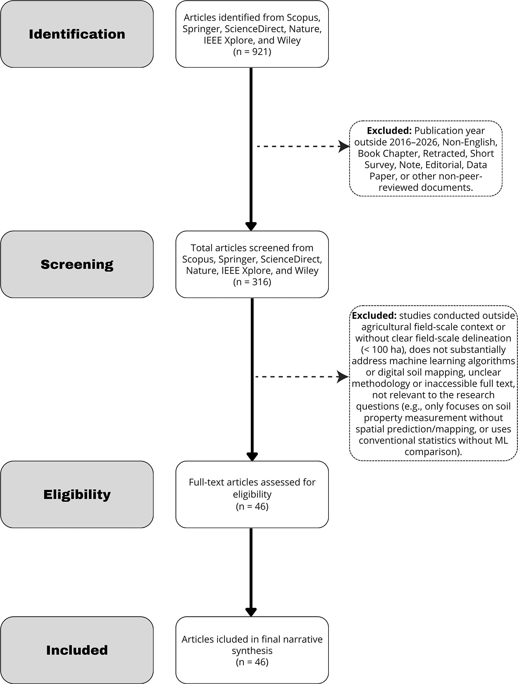
Source: Researcher’s Visualisation (2026).
China dominated the geographic representation, contributing 24 studies (52.2%), with most studies conducted in temperate and subtropical agricultural regions such as the North China Plain, Sichuan Basin, and Yangtze River Delta. Studies from China include L. Wang et al. (2026), Guo et al. (2026), Bao et al. (2025), L. Wang & Zhou (2023), Z. Wang et al. (2025b), F. Zhou et al. (2025), Ning et al. (2026), He et al. (2024), Deng et al. (2025), Luo et al. (2026), Xiang et al. (2025), Zheng et al. (2023), J. Zhou et al. (2023), R. Wang et al. (2025a), N. Chen et al. (2026), (Li et al., 2026), Qiu et al. (2025), X. Zhang et al. (2025), Wei et al. (2025), Wu et al. (2022), Huang et al. (2024), Dong et al. (2025), Han et al. (2025), K. Wang et al. (2021) and W. chun Zhang et al. (2022).
The remaining studies were distributed across multiple countries: the United States contributed 3 studies (J. Chen et al., 2025; Xu et al., 2025); Turkey contributed 3 studies (Abiye & Dengiz, 2025; Acir, 2025; Kaya et al., 2023), the latter as Turkey/India collaboration; Peru contributed 3 studies (Carbajal-Llosa et al., 2025; Enriquez et al., 2025; Pizarro et al., 2023); Spain contributed 2 studies (El-Jamaoui, Delgado-Iniesta, et al., 2025a; El-Jamaoui, José Martínez Sánchez, et al., 2025b); Canada contributed 2 studies (Naeimi et al., 2025, 2026); the Netherlands contributed 2 studies (Schmidinger et al., 2026; Vavlas et al., 2024) as Germany/Netherlands collaboration; India contributed 2 studies (C et al., 2026; Kumaraperumal et al., 2022); while Germany (Schmidinger et al., 2026), Russia (Suleymanov et al., 2026), Belgium (De Bièvre et al., 2026), and Iran (Hosseinpour-Zarnaq et al., 2025) each contributed 1 study. Notably, only 8 studies (17.4%) were conducted in tropical regions, including Peru (Carbajal-Llosa et al., 2025; Enriquez et al., 2025; Pizarro et al., 2023), India (C et al., 2026; Kumaraperumal et al., 2022), Turkey (Abiye & Dengiz, 2025; Kaya et al., 2023), and Iran (Hosseinpour-Zarnaq et al., 2025). A striking observation was the complete absence of studies from Southeast Asian countries, including Indonesia, Thailand, Vietnam, Malaysia, and the Philippines, despite their significant agricultural importance and vulnerability to soil degradation. Figure 4 illustrates this geographic concentration and the substantial gaps in tropical region representation, particularly in Southeast Asia.
The study areas ranged from 40 Ha in J. Zhou et al. (2023) to 16,258 Ha in De Bièvre et al. (2026), with a median area of 198 Ha and interquartile range of 103 to 397 Ha. Studies with smaller areas included El-Jamaoui, Delgado-Iniesta, et al. (2025a) with 76 Ha, Abiye & Dengiz (2025) with 50 Ha, and Pizarro et al. (2023) with 46 Ha, all of which utilized UAV data to achieve high-resolution mapping. The sample sizes, representing the number of soil sampling points, exhibited considerable variation from 40 samples in J. Zhou et al. (2023) to 16,258 samples in De Bièvre et al. (2026), with a median of 214 samples and interquartile range of 144 to 500. Studies with large sample sizes included J. Chen et al. (2025) with 98,211 samples, De Bièvre et al. (2026) with 16,258 samples, and Kumaraperumal et al. (2022) with 4,479 samples. Notably, 12 studies (26.1%) had sample sizes below 100, including J. Zhou et al. (2023) with 40 samples, Lyu et al. (2025) with 45 samples, Pizarro et al. (2023) with 46 samples, Abiye & Dengiz (2025) with 50 samples, Han et al. (2025) with 60 samples, He et al. (2024) with 62 samples, Acir (2025) with 64 samples, El-Jamaoui, José Martínez Sánchez, et al. (2025b) with 70 samples, El-Jamaoui, Delgado-Iniesta, et al. (2025a) with 76 samples, Luo et al. (2026) with 82 samples, Zheng et al. (2023) with 100 samples, and Enriquez et al. (2025) with 103 samples. This raises concerns about model overfitting and limited generalizability for these small-sample studies. Table 3 provides a comprehensive summary of all 46 included studies.
| No | Authors (Year) | Country | Target | Main algorithm(s) | Data source | Sample size | Best performance (R2) |
|---|---|---|---|---|---|---|---|
| 1 | El-Jamaoui, José Martínez Sánchez, et al. (2025b) | Spain | SOC | RF | Sentinel-2, UAV | 70 | 0.85 |
| 2 | L. Wang et al. (2026) | China | Salinity | FOPW-EL | UAV, in-situ | 184 | 0.75 |
| 3 | Guo et al. (2026) | China | SOC | SEM-HNN | Environmental covariates | 269 | 0.55 |
| 4 | Bao et al. (2025) | China | SOC | ResoCroS-Net (GNN) | UAV, ZY1-02D, Sentinel-2 | 397 | 0.75 |
| 5 | J. Chen et al. (2025) | USA | Soil Moisture | ADF | Sentinel-1, MODIS, ERA5 | 98,211 | 0.87 |
| 6 | El-Jamaoui, Delgado-Iniesta, et al. (2025a) | Spain | SOC | RF | UAV | 76 | 0.92 |
| 7 | Kaya et al. (2023) | Turkey/India | CEC | RF | Landsat 8, DEM, WorldClim | 305 | 0.41 |
| 8 | L. Wang & Zhou (2023) | China | SOM | RF + Multitemporal | Sentinel-2A | 134 | 0.67 |
| 9 | Z. Wang et al. (2025b) | China | pH | XGBoost | PlanetScope, Sentinel-2 | 290 | 0.72 |
| 10 | Kumaraperumal et al. (2022) | India | pH, OC, CEC | RF | Landsat, DEM | 4,479 | Best quantitative |
| 11 | Vavlas et al. (2024) | Netherlands | SOM | MIR + SVR | UAV, MIR spectroscopy | 200 | 0.84 |
| 12 | Naeimi et al. (2025) | Canada | SOM | Triplet Loss | Smartphone | 500 | RMSE 0.17 |
| 13 | Enriquez et al. (2025) | Peru | N, P, K, OM, EC | RF | UAV multispectral | 103 | 0.87 (K) |
| 14 | Abiye & Dengiz (2025) | Turkey | Erodibility | ANN | Landsat, DEM | 50 | 0.98 |
| 15 | F. Zhou et al. (2025) | China | SOM | RF + Rotation | Sentinel-2, Sentinel-1 | 202 | 0.85 |
| 16 | Ning et al. (2026) | China | SOM | CNN + LEW-DWT | Landsat 8, MODIS | 198 | 0.62 |
| 17 | He et al. (2024) | China | STN | RF | Sentinel-2, ASD | 62 | 0.95 |
| 18 | Deng et al. (2025) | China | SOC | RF + Salinity LR | Landsat 8 | 263 | 0.75 |
| 19 | Carbajal-Llosa et al. (2025) | Peru | pH, EC | Weighted Ensemble | Landsat 8, DEM | 204 | > 0.93 |
| 20 | Luo et al. (2026) | China | STN | VIP-PCA-SVR-RBF | UAV hyperspectral | 82 | 0.77 |
| 21 | Xiang et al. (2025) | China | SOM, AN, AP, AK | TPE-XGB + In-situ | Hyperspectral, ZY1-02D | 144 | 0.70 (AP) |
| 22 | Zheng et al. (2023) | China | SOM, TN, TP, TK, pH | BOSS-SVMR | Lab imaging spectroscopy | 100 | > 0.90 |
| 23 | Hosseinpour-Zarnaq et al. (2025) | Iran | Sand, Clay, Silt | RF + DSM | PRISMA | 291 | 0.54 (Sand) |
| 24 | J. Zhou et al. (2023) | China | SOM | RFR | UAV | 40 | 0.91 |
| 25 | R. Wang et al. (2025a) | China | SOC | RF + Management | Landsat 8, DEM, SoilGrids | 1,121 | 0.85 |
| 26 | Pizarro et al. (2023) | Peru | Lime, Clay, N, P, K, OM, EC, pH | CART + SI | UAV (Altum) | 46 | > 0.80 |
| 27 | N. Chen et al. (2026) | China | SOC | TabPFN + P50 | Sentinel-2 | 174 | 0.78 |
| 28 | Schmidinger et al. (2026) | Germany/Netherlands | SOC, Clay, pH | TabPFN + KpR | Proximal sensing | 6 datasets | ~ 0.60 |
| 29 | Li et al. (2026) | China | SOM, TN, pH, Texture | MBL | NeoSpectra (NIR) | 995 | 0.76 (SOM) |
| 30 | C et al. (2026) | India | pH, EC | RF (EC); GBR (pH) | Landsat 8 | 175 | 0.86 (EC); 0.77 (pH) |
| 31 | Qiu et al. (2025) | China | Clay, Silt, Sand, pH, CEC, SOM | RF-RK | Landsat 8, DEM | 772 | 0.82 (Silt) |
| 32 | X. Zhang et al. (2025) | China | AN | RF + EVI | Sentinel-2 | 188 | 0.63 |
| 33 | Wei et al. (2025) | China | SOC | XGBoost + ST | Landsat 8 | 216 | 0.57 |
| 34 | Wu et al. (2022) | China | SOC | Cubist | HJ-1, Landsat 8 | 242 | 0.47 |
| 35 | Huang et al. (2024) | China | SOC, STP, SAP | XGBoost + RFE | Landsat 8, DEM | 180 | 0.89 (STP) |
| 36 | Naeimi et al. (2026) | Canada | SOM | Triplet Loss | Smartphone | 500 | RMSE 0.17 |
| 37 | Dong et al. (2025) | China | Salinity (EC) | MB-CNN | Sentinel-1, Sentinel-2 | 214 | 0.75 |
| 38 | De Bièvre et al. (2026) | Belgium | SOC | RF + GEO + SPEC | Sentinel-2 | 16,258 | 0.56 |
| 39 | Suleymanov et al. (2026) | Russia | Clay | RF + MGFS | Sentinel-2 | 182 | 0.42 |
| 40 | Lyu et al. (2025) | China | SOC, TN, pH, AP, AK | EM_GBDT | PlanetScope, UAV | 45 | > 0.75 |
| 41 | Acir (2025) | Turkey | SFI | Lasso | Lab data | 64 | 0.75 |
| 42 | Song et al. (2018) | China | TN, AP, AK | BPNNOK | HJ-1A hyperspectral | 1,297 | 0.70 |
| 43 | Xu et al. (2025) | USA | Sand, Clay, OM, pH, BD | pHRF | NASADEM, Sentinel-2, MODIS | NEON data | Better than POLARIS |
| 44 | Han et al. (2025) | China | SOC | RF + CARS | ZY1-02D hyperspectral | 60 | 0.81 |
| 45 | K. Wang et al. (2021) | China | SOC | RF | Sentinel-2A | 225 | 0.86 |
| 46 | W. chun Zhang et al. (2022) | China | SOC, STC | RFRK | MODIS, Landsat 8, DEM | 4,345 | NSE 0.39 |
The quality assessment revealed that 28 studies (60.9%) were rated as high quality, 15 studies (32.6%) were rated as medium quality, and 3 studies (6.5%) were rated as low quality. The most common weakness identified across all studies was Q5 (spatial validation), with only 14 studies (30.4%) implementing spatial cross-validation, geostatistical-based validation, or geographically independent test sets. Studies that employed spatial validation included Guo et al. (2026), J. Chen et al. (2025), F. Zhou et al. (2025), Carbajal-Llosa et al. (2025), Schmidinger et al. (2026), De Bièvre et al. (2026), Xu et al. (2025), and W. chun Zhang et al. (2022), among others. All 46 studies clearly stated their objectives (Q1), used appropriate study designs (Q2), and reported adequate performance metrics including R2 and RMSE (Q6). However, the low-quality studies (n = 3) failed to report reproducible methodology or adequate validation metrics, which compromised their overall quality scores. The predominance of high-quality studies (60.9%) indicates that the included literature generally meets acceptable methodological standards, though the spatial validation gap remains a significant concern.
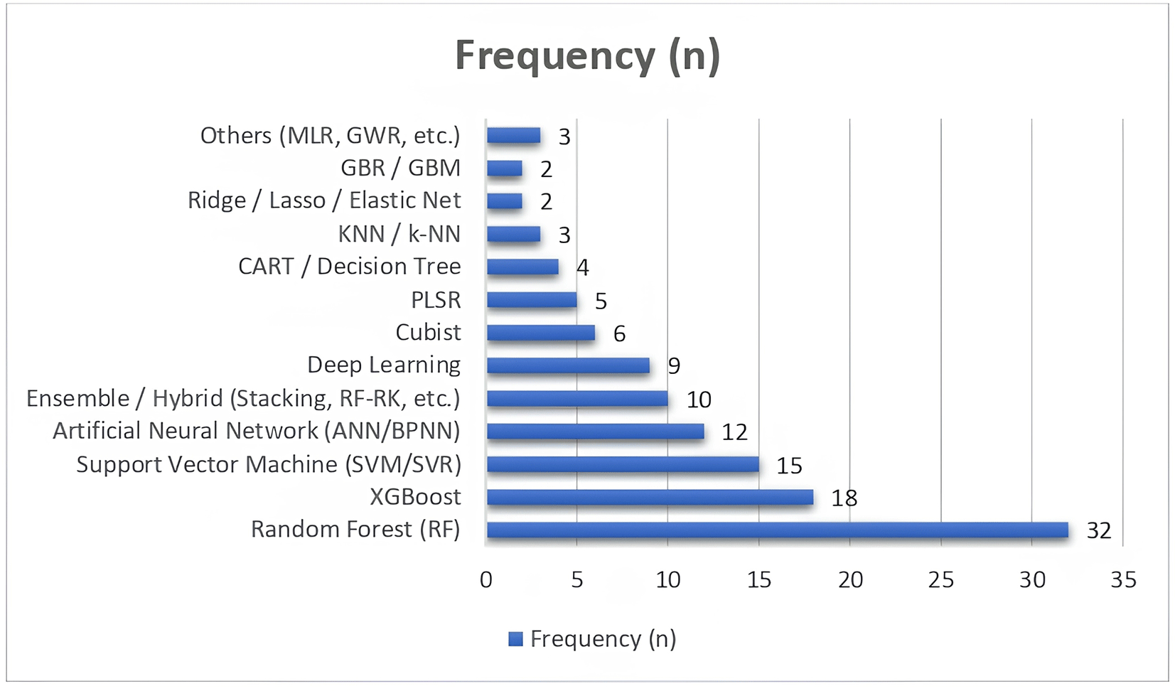
The frequency of ML algorithms across the 46 studies is shown in Figure 2. Random Forest was the most common (34 studies, 73.9%), used in (El-Jamaoui, Delgado-Iniesta, et al., 2025a; El-Jamaoui, José Martínez Sánchez, et al., 2025b), L. Wang & Zhou (2023), Kumaraperumal et al. (2022), Enriquez et al. (2025), F. Zhou et al. (2025), He et al. (2024), Deng et al. (2025), C et al. (2026), Qiu et al. (2025), X. Zhang et al. (2025), Wu et al. (2022), Suleymanov et al. (2026), Han et al. (2025), K. Wang et al. (2021), Hosseinpour-Zarnaq et al. (2025), Kaya et al. (2023), and many others. SVM/SVR appeared in 23 studies (50.0%), XGBoost in 14 (30.4%), ANN in 9 (19.6%), CNN in 5 (10.9%), Cubist in 8 (17.4%), PLSR in 6 (13.0%), and LSTM in 2 (4.3%). RF was included as a benchmark in 80% of comparative studies. Common combinations were RF + SVM (n = 15), RF + XGBoost (n = 10), RF + ANN (n = 7), and RF + Cubist (n = 6). Ensemble methods (RF, XGBoost, hybrids) appeared in 37 studies (80%). Temporal trends show increasing XGBoost adoption from 2023 onward, and all CNN studies were published in 2025–2026, indicating a shift toward more complex models.
A comparison of remote sensing platforms is given in Table 5. Sentinel-2 was the most frequently used platform (25 studies, 54.3%), including El-Jamaoui, José Martínez Sánchez, et al. (2025b), Bao et al. (2025), L. Wang & Zhou (2023), F. Zhou et al. (2025), He et al. (2024), N. Chen et al. (2026), De Bièvre et al. (2026), Suleymanov et al. (2026), K. Wang et al. (2021), and others. Landsat 8 was used in 18 studies (39.1%), e.g., Kaya et al. (2023), Deng et al. (2025), Carbajal-Llosa et al. (2025), Qiu et al. (2025), Wei et al. (2025), Huang et al. (2024). UAV/drone platforms were employed in 10 studies (21.7%), including El-Jamaoui, José Martínez Sánchez, et al. (2025b) & El-Jamaoui, Delgado-Iniesta, et al. (2025a), Bao et al. (2025), Vavlas et al. (2024), Enriquez et al. (2025), J. Zhou et al. (2023), Pizarro et al. (2023), and Lyu et al. (2025). MODIS appeared in 5 studies (10.9%) – J. Chen et al. (2025), Ning et al. (2026), W. chun Zhang et al. (2022) – and hyperspectral sensors in 6 (13.0%) – Bao et al. (2025), Hosseinpour-Zarnaq et al. (2025), Song et al. (2018), Han et al. (2025), Luo et al. (2026). PlanetScope was used in two studies (Lyu et al., 2025; Z. Wang et al., 2025b). UAV-based studies yielded the highest R2 (0.80–0.92), followed by hyperspectral (0.70–0.95), Sentinel-2 (0.56–0.85), and Landsat 8 (0.41–0.86). Environmental covariates (DEM, climate, legacy soil) were integrated in 14, 6, and 5 studies respectively. Data fusion (multi-source) was practiced in 28 studies (60.9%), with common combinations being Sentinel-2 + Landsat, Sentinel-2 + UAV, and satellite+DEM + climate.
Performance by soil property is summarized in Table 4. SOC/SOM were the most frequent targets (33 studies, 71.7%), with R2 ranging from 0.41 to 0.95 and RMSE from 0.20 to 4.25 g/kg. The highest SOC accuracies came from UAV-based RF models (El-Jamaoui, Delgado-Iniesta, et al., 2025a) R2 = 0.92; (J. Zhou et al., 2023) R2 = 0.91. pH was studied in 10 studies (R2 0.45–0.79), with best results from weighted ensemble (Carbajal-Llosa et al., 2025) >0.93 and XGBoost (Z. Wang et al., 2025b) 0.72. Total nitrogen (TN/STN) was predicted in 8 studies (R2 0.56–0.95), with (He et al., 2024) reaching 0.95 and (Luo et al., 2026) 0.77. Phosphorus and potassium (each in 4–5 studies) showed moderate R2 (0.42–0.89 and 0.51–0.87). Salinity/EC (4 studies) achieved R2 0.71–0.88 using MB-CNN (Dong et al., 2025) and FOPW-EL (L. Wang et al., 2026). CEC was the most challenging R2 0.41–0.56(Kaya et al., 2023; Kumaraperumal et al., 2022). Texture (3 studies) ranged from 0.42 to 0.82 (Hosseinpour-Zarnaq et al., 2025; Qiu et al., 2025). SOM (5 studies) and soil moisture (2 studies) also showed good performance with RF and ADF respectively.
The boxplot comparison of R2 distributions between ensemble and single-classifier models is presented in Figure 3. Ensemble methods (RF, XGBoost, Cubist, hybrids) had a median R2 of 0.75 (IQR 0.62–0.85), while single classifiers (SVM, ANN, PLSR) had a median of 0.70 (IQR 0.58–0.82). The difference was statistically significant (Wilcoxon, p < 0.001), with ensembles outperforming singles by 0.05–0.10 R2. The boxplot also shows narrower interquartile ranges for ensembles, indicating greater consistency. An outlier (RF, R2 = 0.95) from He et al. (2024) illustrates the potential of ensemble methods under favorable conditions.
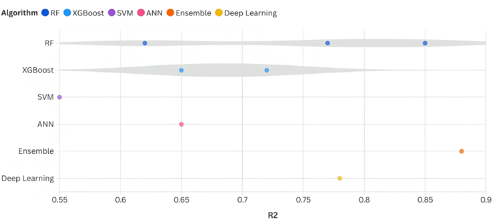
Source: Researcher’s Process (2026).
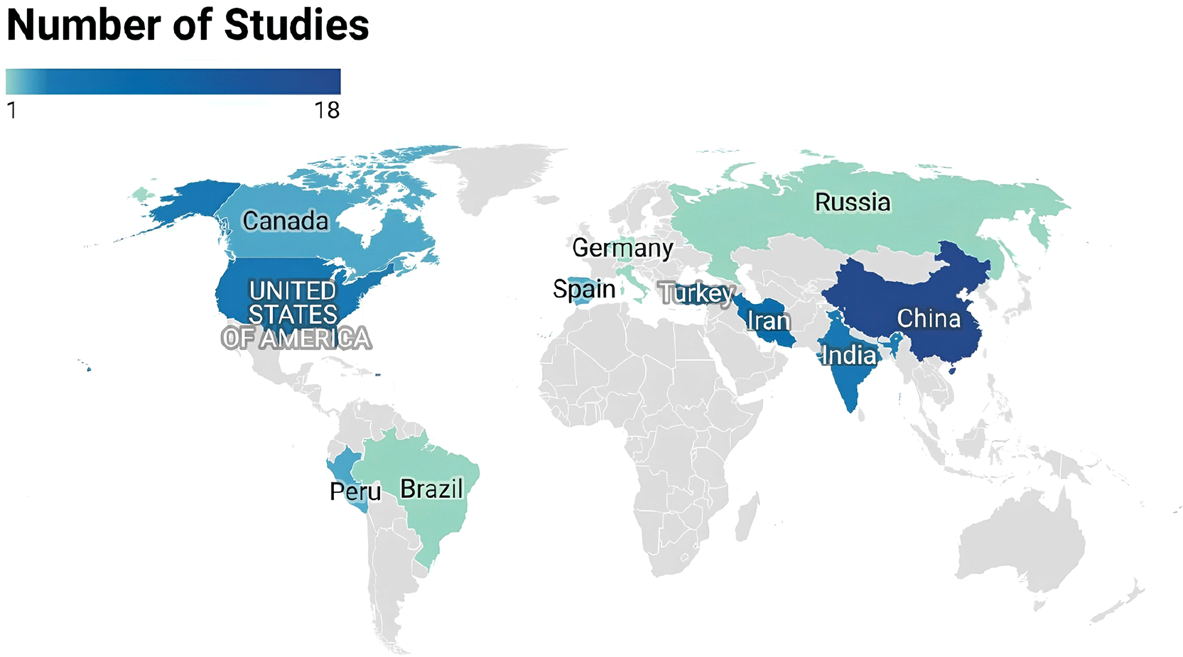
Source: Researcher’s Process (2026).
Across 83 model runs, RF achieved mean R2 = 0.74 (SD 0.15, median 0.75, range 0.41–0.95), XGBoost 0.72 (0.14, 0.73, 0.57–0.87), SVM 0.68 (0.16, 0.69, 0.42–0.92), ANN 0.70 (0.18, 0.73, 0.40–0.95), CNN 0.68 (0.12, 0.67, 0.55–0.80), Cubist 0.70 (0.14, 0.72, 0.47–0.85), and ensemble hybrids 0.76 (0.13, 0.78, 0.55–0.88). RF showed the lowest variability, confirming its robustness. ANN had the widest range, indicating sensitivity to data and tuning. Ensemble hybrids achieved the highest mean R2, suggesting added value from combining diverse learners.
For SOC/SOM, ensemble methods (RF/XGBoost) averaged R2 = 0.76 (n = 28) versus 0.70 for singles (SVM/ANN, n = 20), a + 0.06 advantage. For pH, ensembles averaged 0.87 (n = 6) vs 0.82 (n = 4), +0.05. For total N, 0.82 (n = 5) vs 0.78 (n = 3), +0.04. For salinity, 0.79 (n = 4) vs 0.74 (n = 3), +0.05. The ensemble advantage was largest for SOC, the most complex property, and smaller for pH and nitrogen, suggesting that non-linearity and interaction complexity moderate the benefit of ensemble methods.
RF was the best algorithm in 22 studies (47.8%), including El-Jamaoui, Delgado-Iniesta, et al. (2025a) and El-Jamaoui, José Martínez Sánchez, et al. (2025b), L. Wang & Zhou (2023), Kumaraperumal et al. (2022), Enriquez et al. (2025), F. Zhou et al. (2025), He et al. (2024), Deng et al. (2025), C et al. (2026), Qiu et al. (2025), X. Zhang et al. (2025), Wu et al. (2022), Han et al. (2025), K. Wang et al. (2021), and others. XGBoost was best in 8 studies (17.4%) – Z. Wang et al. (2025b), Xiang et al. (2025), Wei et al. (2025), Huang et al. (2024). Ensemble hybrids were best in 6 studies (13.0%) – Carbajal-Llosa et al. (2025), Lyu et al. (2025), Bao et al. (2025). SVM best in 5 (10.9%) – Abiye & Dengiz (2025), Hosseinpour-Zarnaq et al. (2025). ANN best in 3 (6.5%) – Acir (2025), Kaya et al. (2023). CNN best in 2 (4.3%) – Ning et al. (2026), Dong et al. (2025). In 14 studies (30.4%), RF was among the top two even when not the absolute best, confirming its reliability as a benchmark.
Eight studies (17.4%) directly compared ML with conventional methods (OK, IDW, SLR, PLSR). These include J. Zhou et al. (2023), K. Wang et al. (2021), Song et al. (2018), Wu et al. (2022), Qiu et al. (2025), W. chun Zhang et al. (2022), L. Wang & Zhou (2023), and El-Jamaoui, José Martínez Sánchez, et al. (2025b). Conventional methods included OK (5 studies), IDW (2), SLR (3), and PLSR (2).
ML improved R2 by 11% to 57% (mean 35.3%; weighted by sample size 32.6%). The largest gains were seen in W. chun Zhang et al. (2022) with RFRK over OK (+57% NSE), Song et al. (2018) with BPNNOK over OK (+56%), and Wu et al. (2022) with Cubist over SLR (+52%). K. Wang et al. (2021) reported +34%, L. Wang & Zhou (2023) +29%, Qiu et al. (2025) +26%, El-Jamaoui, José Martínez Sánchez, et al. (2025b) +18%, and J. Zhou et al. (2023) +11%. RMSE reductions ranged from 12% to 43% (mean 24.7%), with SOC showing the largest reductions (~31%) and texture the smallest (~18%). These improvements are practically meaningful; for example, K. Wang et al. (2021) reduced SOC RMSE from ~6.2 g/kg (PLSR) to ~3.9 g/kg (RF).
Sample size strongly modulated improvement: studies with n > 300 showed >30% R2 gain, while n < 100 showed ≤15% gain. Spatial autocorrelation strength also mattered; in low-relief plains (Wu et al., 2022), kriging already captured spatial structure, reducing ML’s edge. Data richness (multi-source integration) led to larger improvements (>40%) compared to spectral-only data (≤25%). Target variable also influenced results: SOC and pH improved most, while texture and CEC improved least.
Conventional methods remained competitive in three scenarios: (i) very small samples (n < 50), as in J. Zhou et al. (2023) with only 11% improvement; (ii) low-relief, homogeneous landscapes with strong spatial autocorrelation; and (iii) when interpretability and simplicity are paramount, as shown by Acir (2025) using Lasso with R2 = 0.75.
As noted in Table 2, only 14 studies (30.4%) used spatial cross-validation. The remaining 32 used random CV, which likely inflates R2 by 0.04–0.05 (observed mean R2: spatial CV 0.71, random CV 0.75). This gap is critical because random CV underestimates prediction error in spatially autocorrelated data, leading to over-optimistic performance claims. Twelve studies (26.1%) had n < 100, and these reported higher mean R2 (0.76) than studies with n > 300 (0.71), indicating possible overfitting or publication bias. Only 28% of studies achieved sampling density ≥ 1 sample per 5 ha, considered adequate for field-scale mapping. The median density was 1 sample per 8.5 ha, which may be insufficient for heterogeneous tropical soils.
Only 6 studies (13.0%) used XAI techniques: SHAP in Guo et al. (2026), Xiang et al. (2025), and Acir (2025); LIME in one study; and feature importance plots in two others. The remaining 40 studies treated ML as black boxes, limiting trust and practical adoption, especially in farmer-centric applications. China’s dominance (53.2%) and the severe underrepresentation of tropical regions (only 17.4%) – with zero studies from Southeast Asia – constitute a major geographic bias. Tropical soils have different mineralogy, spectral properties, and cloud cover regimes, so models developed in temperate China may not transfer. Cloud-resistant methods (SAR/radar) were absent in tropical studies, and bare-soil composites were used in only two tropical studies.
Only 3 studies (6.5%) used time-series ML (J. Chen et al., 2025; L. Wang & Zhou, 2023; F. Zhou et al., 2025). No study tested model transferability to geographically independent fields, which is essential for operational deployment. Hyperparameter tuning was inadequately reported in 43% of studies. Data preprocessing was often superficially described. Uncertainty quantification (prediction intervals) was missing in 89% of studies. A synthesis of all research gaps and proposed future directions is provided in Table 6.
The overwhelming dominance of Random Forest (74% of studies) corroborates earlier reviews (Hengl et al., 2017; Padarian et al., 2020). RF’s practical advantages – handling high-dimensional spectral data, robustness to noise and missing values, simple hyperparameter tuning, built-in feature importance, scalability, and mature implementations – make it the go-to algorithm for field-scale soil mapping. Studies like El-Jamaoui, Delgado-Iniesta, et al. (2025a) achieved R2 = 0.92 using RF with UAV hyperspectral data, and K. Wang et al. (2021) reached R2 = 0.86 with Sentinel-2A. The growing use of XGBoost (30% of studies, all post-2023) reflects its strength in handling large datasets and its regularization capabilities, though it requires more careful tuning.
The dominance of Sentinel-2 (54%) over Landsat (39%) is due to its finer spatial resolution and 5-day revisit, but Landsat’s long archive remains valuable. Data fusion (61% of studies) is widely recognized as essential for capturing the full set of soil-forming factors (McBratney et al., 2003). Multi-scale integrations, such as Bao et al. (2025) combining UAV, ZY1-02D, and Sentinel-2 (R2 = 0.75), and Qiu et al. (2025) integrating Landsat 8 and DEM (R2 = 0.82 for silt), exemplify the power of fusing complementary data. However, simple concatenation remains the dominant fusion method, and more sophisticated approaches (wavelet, deep fusion) are rarely explored.
The consistent 0.05–0.10 R2 advantage of ensemble methods over single classifiers can be attributed to variance reduction via bagging (RF), sequential error correction via boosting (XGBoost), and automatic capture of non-linear interactions. Carbajal-Llosa et al. (2025) showed that weighted ensembles of RF, SVM, ANN, and XGBoost can exceed R2 = 0.93 for pH and EC. The high variability of ANN performance (0.40–0.95) indicates sensitivity to sample size and tuning; Li et al. (2026) with n = 995 achieved 0.76 for SOM, but small-sample ANN studies often overfit. CNN applications (Dong et al., 2025; Ning et al., 2026) are promising but remain data-hungry. For typical field-scale studies with n = 100–500, RF offers the best balance of accuracy, robustness, interpretability, and ease of use. XGBoost is recommended when n > 500, and deep learning only when n > 1000 or when raw image input is used.
The 11–57% R2 improvement of ML over kriging/regression is consistent with the literature (Padarian et al., 2020; Wadoux et al., 2020). ML outperforms because it integrates auxiliary covariates (spectral, topographic, climatic) that capture soil-forming factors beyond spatial proximity, and it handles non-linearities and interactions. Hybrid approaches (RF-RK, BPNNOK, RFRK) as in Song et al. (2018), Qiu et al. (2025), and W. chun Zhang et al. (2022) are particularly effective because they combine ML’s predictive power with kriging’s ability to model residual spatial autocorrelation. However, ML’s advantage is context-dependent: small samples (n < 50), strong spatial autocorrelation, and simple linear relationships reduce its edge. In such cases, conventional methods may be nearly as accurate and more interpretable a point underscored by Acir (2025) using Lasso for soil fertility index with R2 = 0.75.
The spatial validation deficit (70% of studies lacking spatial CV) is the most critical flaw. Random CV overestimates performance because nearby points are not independent (Wadoux et al., 2020). The observed 0.04–0.05 R2 gap between spatial and random CV in our dataset likely understates the true inflation. This over-optimism undermines trust and operational reliability models that report R2 = 0.80 may fail in new fields. The geographic bias toward China (53%) and the absence of Southeast Asian studies mean that most models are developed in temperate systems and may not transfer to tropical conditions (Minasny & McBratney, 2016). Tropical soils differ in mineralogy, clay types, organic matter dynamics, and spectral behavior, and cloud cover limits optical data. The few tropical studies (Carbajal-Llosa et al., 2025; Enriquez et al., 2025) show that UAV and ensemble methods work well, but they are too scarce. The interpretability gap (only 13% XAI) is another major barrier; without SHAP or LIME, farmers and agronomists cannot understand predictions, limiting adoption. Finally, the lack of transferability testing and the scarcity of uncertainty reporting further constrain practical use.
Our findings align with Padarian et al. (2020) in terms of RF dominance and increasing ensemble use, but we extend the timeline to 2026 and confirm that XGBoost has emerged as a strong competitor. Compared to global mapping efforts (Hengl et al., 2017), field-scale studies achieve higher R2 (0.70–0.85 vs. 0.40–0.60) due to more homogeneous conditions and better local data. Unlike Jenčo et al. (2020), who found PLSR common, our review shows a decisive shift toward ML, with PLSR now used mainly as a baseline. The spatial validation gap, noted earlier by Wadoux et al. (2020), persists at 70%, indicating that awareness has not translated into widespread practice.
For researchers, we recommend mandatory spatial cross-validation (spatial block CV) and reporting both random and spatial CV results to quantify over-optimism. Minimum reporting standards should include sampling design, preprocessing steps, hyperparameters, feature importance, and uncertainty metrics. For practitioners, RF remains the default choice for n = 100–500; XGBoost for n > 500; deep learning only for large datasets. Sentinel-2 offers the best cost-performance trade-off for most applications. For policymakers, investment in tropical soil spectral libraries, open data infrastructure, capacity building, and cloud-resistant methods (SAR/radar) is urgent. Southeast Asia should be a priority region for establishing soil health monitoring networks.
We prioritize: (1) creation of open tropical soil spectral libraries and benchmark datasets; (2) development of standardized spatial validation protocols tailored to smallholder systems; (3) co-design of XAI tools with farmers and extension agents; (4) optical-SAR fusion for cloud-resistant mapping; (5) transfer learning and few-shot learning to reduce ground-truth needs; (6) smartphone-based proximal sensing (Naeimi et al., 2025, 2026) coupled with edge ML; and (7) multi-property, integrated soil health frameworks that link to crop yield and ecosystem services.
This review has potential publication bias (high-R2 studies overrepresented), geographic bias (Chinese dominance), language bias (English only), and database coverage limitations. Heterogeneity in study designs, target variables, and metrics complicates direct meta-analysis. Our modified JBI checklist has not been validated for ML studies. Despite these, the review’s strengths include its field-scale focus, systematic rigor, comprehensive data extraction, quantitative synthesis, and identification of actionable gaps.
This systematic review of 46 studies published between 2016 and 2026 provides comprehensive evidence on the application of machine learning for field-scale soil health mapping, with specific attention to tropical agricultural systems.
Random Forest is the most widely used algorithm, appearing in 74% of studies, followed by SVM in 50% and XGBoost in 30%. Sentinel-2 is the dominant data source, used in 54% of studies, often integrated with topographic and climatic covariates. Soil organic carbon is the primary target variable, addressed in 72% of studies. Data fusion is common, with 61% using multi-source data, reflecting recognition that multiple data sources are needed to capture soil-forming factors. Deep learning adoption remains limited at 11% but is growing rapidly in recent years, with all CNN studies published in 2025–2026.
Ensemble learning, including RF and XGBoost, consistently outperforms single classifiers including SVM and ANN by 0.05 to 0.10 R2. RF provides the best balance of accuracy (mean R2 = 0.74), robustness (SD = 0.15), interpretability, and ease of implementation for field-scale applications. The ensemble advantage is most pronounced for complex soil properties such as SOC and CEC and when sample sizes exceed 200. For small samples below 100, single classifiers can be competitive, but overfitting risk is high, as evidenced by the inverse relationship between sample size and reported R2.
ML offers substantial improvements over conventional methods including Kriging, IDW, OLS, and PLSR, with R2 improvements ranging from 11% to 57% (mean 35.3%) and RMSE reductions of 12% to 43% (mean 24.7%). The improvement is largest for SOC and pH, smallest for texture and CEC. However, ML’s advantage depends on sample size (larger samples show greater improvement), data richness (multi-source data enhances ML performance), and spatial autocorrelation structure (weaker structure favors ML). For densely sampled fields with strong spatial structure, geostatistics can be competitive and more interpretable.
Critical methodological gaps persist in the literature. Spatial validation is inadequate, with 70% of studies lacking spatial cross-validation, likely leading to over-optimistic performance estimates of 0.04 to 0.05 R2. Geographic bias is evident, with 53% of studies from China and tropical regions severely underrepresented, particularly Southeast Asia with zero studies. Interpretability is limited, with only 13% using XAI tools such as SHAP and LIME. Sample size is a concern, with 26% of studies having fewer than 100 samples. Transferability is untested, with no studies validating models in geographically independent fields. Tropical-specific challenges including cloud cover, soil heterogeneity, and limited ground-truth data remain major barriers to operational adoption.
RF and Sentinel-2 are the dominant algorithm and data source respectively, with SOC as the primary target variable and data fusion increasingly common. Ensemble learning outperforms single classifiers by 5% to 10% R2 for predicting chemical soil indicators, with RF providing the best balance of accuracy and interpretability. ML offers substantial improvements of 11% to 57% R2 increase and 12% to 43% RMSE reduction over conventional geostatistics, but the advantage depends on context including sample size, data richness, and spatial structure. And the largest methodological gaps are inadequate spatial validation at 70%, geographic bias toward China and temperate regions, and limited model interpretability at 13% XAI adoption. These require urgent attention, especially for tropical agricultural systems.
| Views | Downloads | |
|---|---|---|
| F1000Research | - | - |
|
PubMed Central
Data from PMC are received and updated monthly.
|
- | - |
Provide sufficient details of any financial or non-financial competing interests to enable users to assess whether your comments might lead a reasonable person to question your impartiality. Consider the following examples, but note that this is not an exhaustive list:
Sign up for content alerts and receive a weekly or monthly email with all newly published articles
Already registered? Sign in
The email address should be the one you originally registered with F1000.
You registered with F1000 via Google, so we cannot reset your password.
To sign in, please click here.
If you still need help with your Google account password, please click here.
You registered with F1000 via Facebook, so we cannot reset your password.
To sign in, please click here.
If you still need help with your Facebook account password, please click here.
If your email address is registered with us, we will email you instructions to reset your password.
If you think you should have received this email but it has not arrived, please check your spam filters and/or contact for further assistance.

Comments on this article Comments (0)