Solar Irradiation Forecasting Using Genetic Algorithms

Vinodhkumar Gunasekaran; KIRAN KUMAR KOVI; SETHAN ARJA; RAGHUVEER CHIMATA; Ilamathi Elango; Arunkumar Parthasarathy

doi:10.12688/f1000research.176354.1

Home Browse Solar Irradiation Forecasting Using Genetic Algorithms

ALL Metrics

-

Views

Get PDF

Get XML

Export

▬

✚

Research Article

Solar Irradiation Forecasting Using Genetic Algorithms

[version 1; peer review: awaiting peer review]

Vinodhkumar Gunasekaran ¹, KIRAN KUMAR KOVI², SETHAN ARJA², RAGHUVEER CHIMATA³, Ilamathi Elango⁴, Arunkumar Parthasarathy⁵

Vinodhkumar Gunasekaran ¹, KIRAN KUMAR KOVI², [...] SETHAN ARJA², RAGHUVEER CHIMATA³, Ilamathi Elango⁴, Arunkumar Parthasarathy⁵

PUBLISHED 06 Jan 2026

Author details Author details

¹ Global Analytics & Solutions, Circana, Chicago, Illinois, 60606, USA
² VzRAM Tech LLC, Lisle, ILLINOIS, USA
³ GattyInstruments AB, UPSALA, Sweden
⁴ Medline Industries, Northfield, ILLINOIS, 60093, USA
⁵ Customer Solutions for Industries, Oracle, Austin, Texas, 78741, USA

Vinodhkumar Gunasekaran
Roles: Conceptualization, Formal Analysis, Investigation, Methodology, Project Administration, Software, Supervision, Validation

KIRAN KUMAR KOVI
Roles: Resources, Validation, Writing – Original Draft Preparation

SETHAN ARJA
Roles: Software, Validation

RAGHUVEER CHIMATA
Roles: Data Curation, Software, Visualization, Writing – Review & Editing

Ilamathi Elango
Roles: Software, Validation, Writing – Review & Editing

Arunkumar Parthasarathy
Roles: Software, Visualization

OPEN PEER REVIEW

REVIEWER STATUS AWAITING PEER REVIEW

Abstract

Background

For many applications such as photovoltaic system planning, grid stability, and renewable energy integration, accurate forecasting of solar irradiation is essential. Solar irradiation exhibits strong nonlinearity and variability driven by atmospheric conditions, seasonal cycles, and site-specific meteorological factors, making reliable short-term prediction challenging for conventional statistical models.

Methods

We propose a hybrid solar irradiation forecasting framework that combines machine learning regression models with genetic algorithm (GA)–based model optimization. Multiple predictive models, including linear regression and gradient-boosted decision trees, are trained using meteorological variables such as zenith angle, temperature, relative humidity, and atmospheric indices. The GA is employed to identify optimal feature subsets by maximizing predictive accuracy while minimizing redundancy, treating feature selection as a combinatorial optimization problem. Model performance is evaluated using mean absolute error (MAE), variance, and percentage accuracy derived from mean absolute percentage error (MAPE).

Results

The GA-optimized models demonstrate improved forecasting accuracy and stability compared to baseline machine learning approaches using full feature sets. Empirical results show that GA-based feature selection reduces prediction error, enhances robustness across seasonal regimes, and yields interpretable feature importance patterns aligned with known physical drivers of solar irradiation. Comparative evaluation across training and validation datasets confirms consistent gains in predictive performance.

Conclusions

The proposed genetic algorithm–enhanced forecasting framework provides an effective and interpretable approach for modeling solar irradiation under complex atmospheric conditions. By integrating evolutionary optimization with machine learning, the methodology supports more reliable solar energy forecasting and can be readily extended to real-time energy management systems and large-scale renewable deployment scenarios.

Keywords

Solar irradiation, genetic algorithms, XGBoost, machine learning, renewable energy forecasting, solar radiation prediction, feature selection, evolutionary optimization, atmospheric variables, photovoltaic power modeling, time-series regression, nonlinear forecasting, SURFRAD, meteorological data, energy analytics, grid integration, predictive modeling

Corresponding author: Vinodhkumar Gunasekaran

Competing interests: No competing interests were disclosed.

Grant information: The author(s) declared that no grants were involved in supporting this work.

Copyright: © 2026 Gunasekaran V et al. This is an open access article distributed under the terms of the Creative Commons Attribution License, which permits unrestricted use, distribution, and reproduction in any medium, provided the original work is properly cited.

How to cite: Gunasekaran V, KOVI KK, ARJA S et al. Solar Irradiation Forecasting Using Genetic Algorithms [version 1; peer review: awaiting peer review]. F1000Research 2026, 15:12 (https://doi.org/10.12688/f1000research.176354.1) First published: 06 Jan 2026, 15:12 (https://doi.org/10.12688/f1000research.176354.1) Latest published: 06 Jan 2026, 15:12 (https://doi.org/10.12688/f1000research.176354.1)

Introduction

The use of renewable energy worldwide has increased significantly in recent years. Although various renewable energy sources such as wind, tidal, and marine are available, solar energy has the potential to become the most significant renewable resource. Recent advances in technology have improved the efficiency of solar photovoltaic cells while reducing manufacturing costs.^1–3 Accurate forecasting of solar irradiation is critical not only to optimize solar power generation but also to ensure effective grid management and identify alternative power sources when solar energy is unavailable. This is because solar irradiation is crucial for solar power generation.

In recent studies, several machine learning (ML) models have been applied to predict solar irradiation, including Artificial Neural Networks,^4,5 Probabilistic Models,⁶ Bayesian Methods,⁷ Deep Learning Models,^8,9 and Support Vector Machines.¹⁰ In this work, we investigate and validate ML algorithms such as linear regression (LR) and Extreme Gradient Boosting (XGB),^11–13 along with genetic algorithm optimization (GA).^14–17 The data used in this study were obtained from three meteorological stations, Bondville, IL; Desert Rock, NV; and Penn State, PA, that are part of the SURFRAD network.^18,19 These stations were selected for their diverse climatic conditions throughout the year, providing a comprehensive evaluation environment for the models.

The study focuses primarily on predicting the Global Horizontal Irradiance (GHI), a key measure of solar irradiation, and evaluates the potential of Genetic Algorithms to enhance the forecasting accuracy of global solar irradiation. By integrating GA with traditional ML approaches such as LR and XGB, we aim to overcome the challenges associated with manual hyperparameter tuning and improve model robustness. The automated optimization process enabled by GA is particularly valuable in adapting to the nonlinear and dynamic nature of solar irradiation data, ultimately contributing to more reliable predictions.

This research not only demonstrates the superior performance of GA-optimized models but also highlights the broader implications of integrating advanced machine learning techniques into renewable energy forecasting. The findings suggest that the use of a GA approach can lead to significant improvements in prediction accuracy and computational efficiency. This, in turn, has the potential to facilitate better energy management and grid reliability, supporting the ongoing transition toward a more sustainable and resilient energy infrastructure. The acronyms, symbols, and meteorological variables used throughout this study are summarized in Table 1.

Table 1. Nomenclature of acronyms and variables used in this study.

Symbol	Description
Acronyms
GHI	Global Horizontal Irradiance
LR	Linear Regression
XGB	Extreme Gradient Boosting
GA	Genetic Algorithm
GAO	Genetic Algorithm Optimization
MSE	Mean Squared Error
MAE	Mean Absolute Error
Variables
dt	Decimal time
zen	Solar zenith angle ( $^{\circ}$ )
dw solar	Downwelling global solar
uw solar	Upwelling global solar
direct n	Direct-normal solar
diffuse	Downwelling diffuse solar
dw ir	Downwelling thermal infrared
dw casetemp	Downwelling IR case temperature (K)
dw dometemp	Downwelling IR dome temperature (K)
uw ir	Upwelling thermal infrared
uw casetemp	Upwelling IR case temperature (K)
uw dometemp	Upwelling IR dome temperature (K)
uvb	Global UVB
par	Photosynthetically active radiation
netsolar	Net solar (dw solar - uw solar)
netir	Net infrared ( $dw$ ir - uw ir)
totalnet	Net radiation (netsolar + netir)
temp	10-meter air temperature ( $^{\circ} C$ )
rh	Relative humidity (%)
windspd	Wind speed
winddir	Wind direction ( $^{\circ}$ , clockwise from north)
pressure	Station pressure (mb)

Methods

Data preprocessing

Solar irradiation data from the SURFRAD network, measured using a pyranometer, are available for the past 20 years from seven stations in different states of the United States. For this study, data from three stations, Bondville, IL; Penn State, PA; and Desert Rock, NV, were selected due to their distinct climatic conditions throughout the year. The dataset covers three consecutive years from 2018 to 2020, with data from 2018-2019 used for training and data from 2020 used for validation and testing. This selection highlights the geographical variability in solar radiation. Only daytime data, recorded between 7:00 AM and 4:00 PM when solar irradiance is significant, were used, resulting in nine hours of data per day for model development.

The models are designed to predict the Global Horizontal Irradiance (GHI) for the next minute using input parameters such as temperature, pressure, wind speed, wind direction, relative humidity, solar zenith angle, net solar radiation, and time (detailed in minutes, hours, and months). Before training, the data were normalized, outliers were removed, and the dataset was cleaned to ensure a normalized distribution. A few of the parameters can be seen in Figures 1, 2, and 3, with plots showing an example of pre- and post-processed data.

Figure 1. Data preprocessing for dw_solar showing distributions before (left) and after (right) outlier removal.

Extreme placeholder values (e.g., −9999.9) were removed to obtain physically meaningful and normalized distributions for model training.

Figure 2. Data preprocessing for temperature showing distributions before (left) and after (right) outlier removal.

Cleaning and normalization reduce skewness and improve statistical consistency across observations.

Figure 3. Data preprocessing for relative humidity showing distributions before (left) and after (right) outlier removal.

The preprocessing step removes invalid measurements and yields a realistic humidity distribution.

Outlier detection

Outliers were removed as they severely impact the functionality of the model. For example, values such as -9999.90 are recorded for at least 11 variables in the data. Figures 1, 2, and 3 show the data after removing the outliers. Data preprocessing was performed to obtain normalized distributions by removing outliers and cleaning the data. Each row shows the variable before (left) and after (right) preprocessing.

Feature selection

Feature selection removes irrelevant features to enhance model performance by reducing both complexity and computational time. It also eliminates highly collinear variables. In this study, feature selection was performed by evaluating the importance of parameters using the Random Forest method. Out of fifteen variables, eight parameters that showed high relevance to the dependent variable were selected for training the model. Figure 4 illustrates the features deemed most important.

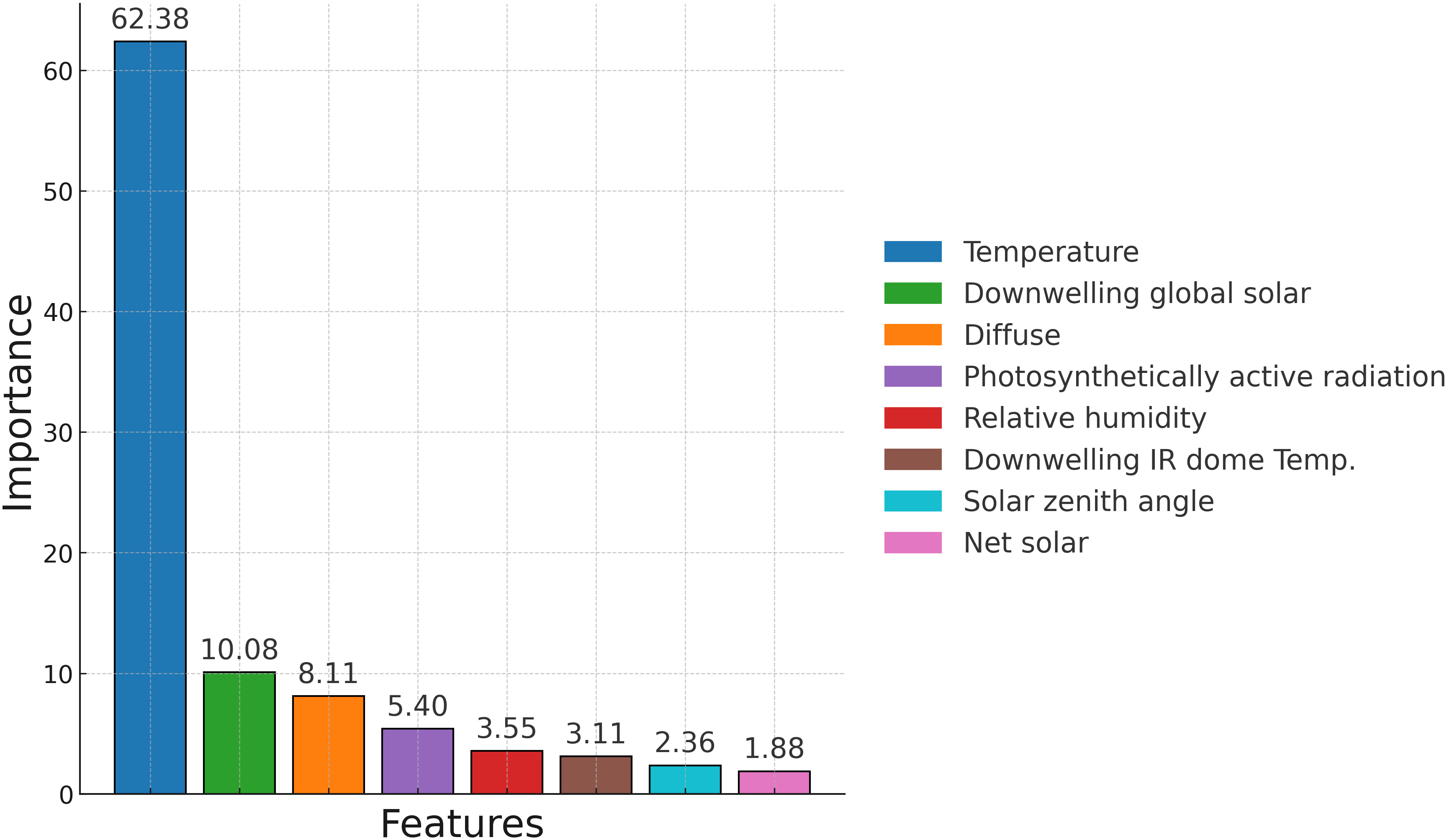
Figure 4. Feature importance used in the feature selection process (Random Forest).

The top eight features are considered for the model. The top eight features—temperature, downwelling global solar radiation, diffuse radiation, photosynthetically active radiation (PAR), relative humidity, downwelling IR dome temperature, solar zenith angle, and net solar radiation—were selected for model training.

Literature review

Linear Regression (LR)

LR is one of the methods used in this study for predicting solar irradiation, where the dependent variable is continuous. LR models the relationship between the dependent variable and one or more independent variables by fitting a linear equation to the observed data. A simple LR equation is expressed as:

y = mx + b

where

y

represents the predicted value,

x

is the input variable,

m

is the slope, and

b

is the intercept.

Extreme Gradient Boosting (XGB)

XGB is a machine learning technique used for both regression and classification tasks. It constructs a predictive model by creating an ensemble of weak learners, typically decision trees, in a stage-wise manner. Like other boosting methods, XGB optimizes an arbitrary differentiable loss function.¹² It uses a partitioning algorithm to identify the optimal data split for a single target variable, and by resampling the data multiple times, it generates a weighted average from these resamples to form the final prediction. This approach, known as tree boosting, builds a series of decision trees into one robust predictive model. Similar to standalone decision trees, boosting does not assume any specific distribution for the data, yet it is less prone to overfitting because it gradually refines the model by combining multiple trees.

Genetic Algorithm (GA)

GA, first introduced by John Holland, is a meta-heuristic search and optimization algorithm inspired by Charles Darwin’s theory of natural selection. In GA, the best solutions are selected from a population and are combined and mutated to produce offspring that are progressively better. In this study, GA is employed to optimize the hyperparameters of the XGB model. This automated approach addresses the challenge of manual hyperparameter tuning, which can be laborious and may not always yield the best configuration for future predictions. By eliminating the need for blind selection, GA naturally improves the model’s accuracy without overfitting.^14,20

Evaluation metric

The performance of these models is evaluated using the mean squared error (MSE), defined as

MSE = \frac{1}{N} \sum_{i = 1}^{N} {(y_{i} - \hat{y_{i}})}^{2}

where

N

is the total number of observations (data points),

y_{i}

is the actual value of an observation, and

\hat{y_{i}}

is the prediction. Descriptive statistics for the input variables used in model training and evaluation are summarized in Tables 2, 3, and 4, providing an overview of the distributional characteristics of radiation, energy balance, and meteorological features. In addition to MSE, model performance is evaluated using mean absolute error (MAE), explained variance, and prediction accuracy derived from mean absolute percentage error (MAPE), which are reported in the results section.

Table 2. Summary statistics for time and radiation variables.

Statistic	dt	zen	dw solar	diffuse	dw ir	dw dometemp	uvb	par
count	156497	156497	156497	156497	156497	156497	156497	156497
mean	14.62	56.97	356.75	152.49	347.08	290.72	51.01	155.32
std	1.48	15.94	271.79	111.52	52.54	9.17	51.85	114.18
min	10.98	20.41	0.10	1.10	209.50	272.14	0.10	0.70
25%	13.48	44.89	119.10	71.50	314.90	282.33	10.50	55.70
50%	14.73	58.75	293.60	118.10	355.00	292.74	30.80	130.50
75%	15.88	69.88	562.40	206.50	389.40	298.26	77.30	243.60
max	16.98	85.00	1356.80	763.70	457.10	309.51	291.60	568.90

Table 3. Summary statistics for solar energy balance variables.

Statistic	netsolar	totalnet	temp
count	156497	156497	156497
mean	283.19	226.03	15.86
std	216.05	188.51	8.71
$min$	0.30	0.10	0.10
25%	96.10	63.20	7.90
50%	232.10	175.20	18.30
75%	442.50	357.70	23.00
max	1112.40	1049.00	32.70

Table 4. Summary statistics for meteorological variables.

Statistic	rh	windspd	winddir	pressure
count	156497	156497	156497	156497
mean	75.09	4.87	180.19	991.33
std	16.48	2.78	95.69	5.76
min	15.10	0.10	0.10	969.40
$25 %$	64.40	2.80	104.00	988.20
$50 %$	77.80	4.30	189.50	991.30
$75 %$	88.40	6.50	250.90	994.90
max	101.30	20.30	360.00	1009.00

Workflow overview

Figure 5 depicts the complete workflow adopted for the development and evaluation of the solar-irradiation forecasting framework. The process begins with the acquisition of minute-resolution meteorological measurements from three geographically diverse SURFRAD stations (Bondville, Illinois; Penn State, Pennsylvania; and Desert Rock, Nevada). The raw observations are subjected to a systematic preprocessing stage, wherein physically implausible records (for example, placeholders such as -9999.9) are identified and removed. The remaining data are subsequently normalized to ensure statistical consistency across variables.

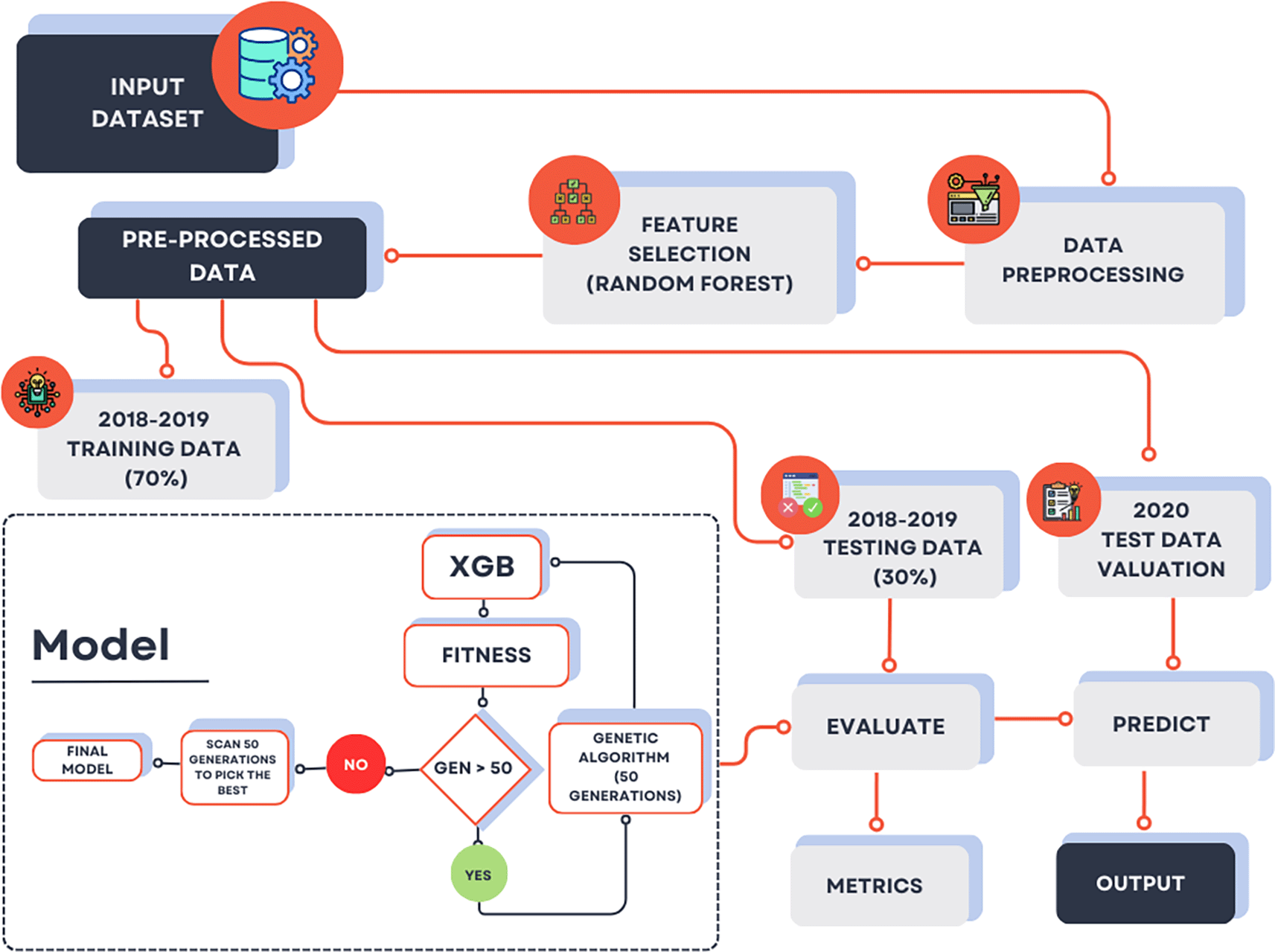
Figure 5. Workflow of the solar irradiation forecasting framework.

The diagram illustrates data acquisition, preprocessing, feature selection, dataset partitioning into training (2018–2019) and validation/testing (2020), model training using Linear Regression (LR), Extreme Gradient Boosting (XGB), and Genetic Algorithm (GA)–optimized XGB, followed by performance evaluation and prediction output.

Following data cleansing, a feature selection procedure based on Random-Forest variable importance is employed to identify the most influential predictors of Global Horizontal Irradiance (GHI).

The curated dataset is then partitioned into training (2018-2019) and validation (2020) subsets to facilitate unbiased model evaluation. Three machine learning approaches are subsequently implemented: (i) Linear Regression (LR) as a baseline statistical model, (ii) Extreme Gradient Boosting (XGB) as an ensemble tree-based learner, and (iii) XGB with Genetic Algorithm (GA)-driven hyperparameter optimization, wherein GA operations of selection, crossover, and mutation iteratively refine the parameter set to achieve near-optimal model performance.

The final stage of the workflow involves quantitative performance assessment of all models on the independent validation set using established metrics-mean squared error (MSE), mean absolute error (MAE), explained variance, and predictive accuracy. The diagram therefore encapsulates the complete end-to-end pipeline, from data acquisition and preprocessing through feature engineering, model training and GA-based optimization, culminating in rigorous validation and comparative performance analysis.

Results and Discussion

The study employed three different machine learning models LR, XGB, and a GA-based approach to predict solar irradiation using datasets from 2018–2019 for model training and internal evaluation respectively. The XGB model was implemented using four different parameter sets to identify the optimal configuration for solar irradiation prediction, while the GA model was explored under three configurations with varying numbers of generations such as: 10, 20 and 50. Each of the varying generations produced results.

Each of the varying GA configurations produced progressively improved performance, with lower-generation settings converging rapidly and higher-generation settings yielding marginal accuracy gains at the expense of increased computational cost. Based on this trade-off between accuracy and efficiency, the GA configuration with 10 generations was identified as the most effective and is therefore used for subsequent comparative analysis.

The overview of the entire workflow is depicted in Figures 6 and 7, which show input data sets, data preprocessing, feature selection, training, testing and validation of data. The flow shows the evaluation and prediction of the model. The XGB is further processed with GA using different generations to improve the model further as can be seen in the flow chart, thereby producing an enhanced model predicting with higher accuracy.

Figure 6. Validation results for the three stations depicting observed Global Horizontal Irradiance (GHI) compared with predictions from Linear Regression (LR), Extreme Gradient Boosting (XGB), and Genetic Algorithm (GA) models for Bondville, IL; Desert Rock, NV; and Penn State, PA during May.

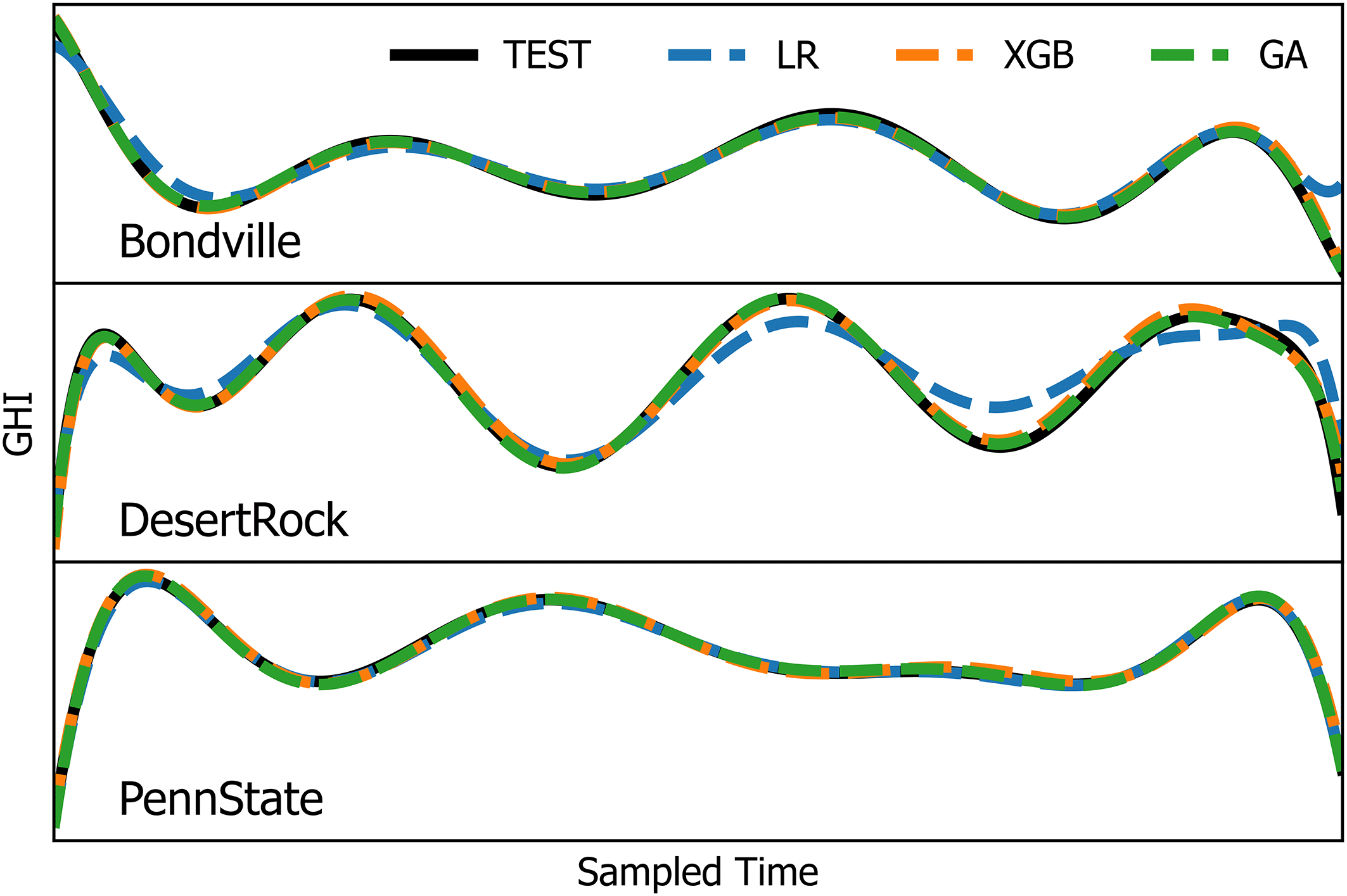
Figure 7. Cross-validation and test results for the three stations depicting observed Global Horizontal Irradiance (GHI) compared with predictions from Linear Regression (LR), Extreme Gradient Boosting (XGB), and Genetic Algorithm (GA) models for Bondville, IL; Desert Rock, NV; and Penn State, PA during May.

A cross-site comparison of model performance is provided in Tables 5, 6, and 7. For each station (Bondville, IL; Desert Rock, NV; and Penn State, PA), we report MAE, explained variance, and overall accuracy for the LR baseline, XGB, and GA-optimized XGB under both Train-Test and Validation splits. Splitting the results by station allows for clearer comparison of model behavior across distinct climatic regimes.

Table 5. Model performance comparison for Bondville, IL.

Metric	LR	XGB-100	GA 10
Train-Test
MAE	14.73	5.39	4.64
Variance	88.19	97.93	98.42
Accuracy (%)	95.55	98.41	98.64
Validation
MAE	14.18	7.69	7.45
Variance	88.23	95.70	95.95
Accuracy (%)	95.63	97.67	97.74

Table 6. Model performance comparison for Desert Rock, NV.

Metric	LR	XGB-100	GA 10
Train-Test
MAE	12.09	5.30	4.58
Variance	90.13	98.00	98.47
Accuracy (%)	96.16	98.32	98.55
Validation
MAE	13.03	12.68	12.92
Variance	89.85	89.43	88.81
Accuracy (%)	95.95	96.04	95.96

Table 7. Model performance comparison for Penn State, PA.

Metric	LR	XGB-100	GA 10
Train-Test
MAE	3.89	3.69	3.08
Variance	98.94	99.01	99.28
Accuracy (%)	98.81	98.61	99.09
Validation
MAE	6.07	5.51	5.42
Variance	97.01	97.91	97.96
Accuracy (%)	98.15	98.30	98.33

Among these, the LR model exhibited the lowest performance, with an accuracy of about $95.5 %$ and a mean absolute error (MAE) of 14.73. Although the XGB model improved upon LR by achieving an accuracy of roughly $98.5 %$ , it still did not match the performance of the GA-enhanced model. The GA model configured with 10 generations produced the best results on the test dataset, attaining an accuracy of $99 %$ with a significantly lower MAE of 2.74. On the validation set, the GA approach also showed strong performance, achieving an accuracy of approximately $97.75 %$ and a MAE of 7.45.

Performance comparisons across different meteorological stations Bondville, IL; Desert Rock, NV; and Penn State, PA show that the GA model consistently outperformed both XGB and LR in the validation phase. For instance, while XGB generally provided better results than LR, an exception was observed at Penn State, PA, where LR marginally outperformed XGB by $0.2 %$ . Nevertheless, across all stations, GA not only achieved the highest accuracy but also demonstrated the lowest MAE; most notably, Penn State recorded an accuracy of $98.33 %$ with a MAE of 5.42.

Beyond its high predictive accuracy, the GA model’s ability to automatically optimize hyperparameters confers significant practical advantages. This automation dramatically reduces the need for extensive manual tuning, saving both time and resources while minimizing human-induced errors in parameter selection. By enabling the model to quickly adapt to different datasets and changing environmental conditions, the GA approach is particularly well-suited for operational forecasting systems that require rapid updates and high reliability.

While the GA-optimized XGB model showed strong performance, there is still room for improvement by expanding the range of hyperparameters used during optimization. For example, testing more values for learning rate, tree depth, and regularization settings could help the model perform better across different weather conditions. Improving the way the genetic algorithm selects the best model-such as by considering both accuracy and consistency-could also make the model more reliable.

As shown in Figures 6 and 7, the GA-based model closely follows observed GHI across test and validation phases for all three stations.

Conclusion

Data collected from three meteorological stations with diverse climatic conditions were used to evaluate the effectiveness of genetic algorithms in enhancing the accuracy of global solar irradiation forecasting. Machine learning techniques such as Linear Regression, Extreme Gradient Boosting, and Genetic Algorithm Optimization were applied and their prediction results compared. The findings demonstrate that the GA-optimized model outperforms the other techniques, delivering superior accuracy across all tested stations. This study provides a basis for assessing the performance of different ML methods for solar irradiation prediction, despite the relatively small sample size. The consistent superiority of the GA approach suggests that automated hyperparameter optimization can significantly improve model performance, making it a promising tool for operational forecasting. Future research should aim to expand the sample size by incorporating data from additional meteorological centers with varying climatic conditions. Furthermore, increasing the number of input parameters and refining the existing parameter set could further enhance the predictive capability of the model.

Limitations and future work

Despite the strong performance achieved by the GA-optimized XGB models, several limitations remain that motivate future research directions. First, the current study evaluates model performance using a limited set of machine learning architectures. GA-based optimization does substantially improve predictive accuracy however, the results may still be sensitive to the choice of the underlying base learner. Including additional gradient-boosting models, such as LightGBM would help with further enhancing robustness across different climatic regimes and patterns. Future work can explore the development of ensemble strategies; these strategies could combine multiple GA-optimized learners using techniques such as stacking, weighted averaging, or meta-learning, that can improve results. Such ensemble approaches also have the potential to reduce model variance and improve generalization, particularly for stations exhibiting highly diverse weather patterns.

Another limitation of the present study is the reliance on a fixed set of meteorological input variables. As additional predictors, such as lagged solar irradiance values, cloud cover indices, aerosol optical depth, or satellite-derived radiative measurements, are included in the study, it may enable the models to better capture rapid atmospheric changes and improve short-term forecasting accuracy. Future extensions could integrate deterministic forecasting frameworks such as the Generalized Adaptive Capped Estimator (GACE), which emphasizes interpretability, stability, and robustness for operational time-series forecasting. GACE has been shown to perform well in environments characterized by structural breaks, volatility, and bounded growth, making it a promising complementary approach for solar irradiation forecasting in real-world energy planning contexts.²¹

Finally, expanding the evaluation to include additional geographic regions, longer temporal horizons, and real-time forecasting scenarios would provide a more comprehensive assessment of model scalability and operational applicability. Addressing these limitations will further strengthen the reliability of machine learning–based solar irradiation forecasting systems and support their deployment in practical renewable energy management applications.

Ethics and consent

No human subjects, private data, or biological specimens were involved.

Data availability

Underlying data

Repository name: Solar Irradiation Forecasting Dataset (SURFRAD, 2018–2020).

https://doi.org/10.5281/zenodo.18056194.²²

The project contains the following underlying data:

• export_dataframe_2018.csv (minute-resolution processed meteorological and solar irradiation data used for model training).
• export_dataframe_2019.csv (minute-resolution processed meteorological and solar irradiation data used for model training).
• export_dataframe_2020.csv (minute-resolution processed meteorological and solar irradiation data used for independent validation).

Data are available under the terms of the Creative Commons Zero “No rights reserved” data waiver (CC0 1.0 Public domain dedication).

Software availability

Source code available from:

https://github.com/vinoalles/SolarIRF

Archived source code available from:

https://doi.org/10.5281/zenodo.18056194

License: The software is released under the MIT License, an OSI-approved open-source license, which permits free use, modification, and redistribution.

Reporting guidelines

This study does not involve clinical trials, human participants, animals, or qualitative research, and therefore does not require CONSORT, STROBE, ARRIVE, or COREQ/SRQR reporting checklists. The article follows the general reproducibility and transparency standards recommended by F1000Research for computational research.

Acknowledgements

The authors acknowledge the developers and contributors of open-source scientific computing and machine learning libraries used in this study.

References

1. Khatib T, Mohamed A, Sopian K: A review of solar energy modeling techniques. Renew. Sust. Energ. Rev. 2012; 16: 2864–2869. Publisher Full Text
2. Lazo JK, Lawson M, Larsen PH, et al.: 300 billion worth of weather: The economic value of weather and climate forecasts. Bull. Am. Meteorol. Soc. 2011; 92: 709–720.
3. Dagne M, David M, Lauret P, et al.: Solar irradiation forecasting: State-of-the-art and future prospects. Renew. Sust. Energ. Rev. 2013; 27: 65–74.
4. Yadav AK, Chandel SS: Solar radiation prediction using artificial neural network techniques: A review. Renew. Sust. Energ. Rev. 2014; 33: 772–781.
5. Chow SKH, Lee EWM, Li DHW: Short-term prediction of photovoltaic energy generation by intelligent approach. Energ. Buildings. 2012; 55: 660–667. Publisher Full Text
6. Fatemi SA, Kuh A, Fripp M: Parametric methods for probabilistic forecasting of solar irradiance. Renew. Energy. 2018; 129: 666–676. Publisher Full Text
7. Lauret P, Boland J, Ridley B: Bayesian statistical analysis applied to solar radiation modelling. Renew. Energy. 2013; 49: 124–127. Publisher Full Text
8. Alzahrani A, Shamsi P, Dagli C, et al.: Solar irradiance forecasting using deep neural networks. Procedia Computer Science. 2017; 114: 304–313. Publisher Full Text
9. Alzahrani A, Shamsi P, Ferdowsi M, et al.: Solar irradiance forecasting using deep recurrent neural networks. Proceedings of the IEEE International Conference on Renewable Energy Research and Applications (ICRERA). 2017; pages 988–994.
10. Wang F, et al.: Solar irradiance feature extraction and support vector machines based weather status pattern recognition model for short-term photovoltaic power forecasting. Energy. 2015; 86: 427–438. Publisher Full Text
11. Fan J, et al.: Comparison of support vector machine and extreme gradient boosting for predicting daily global solar radiation. Energy Convers. Manag. 2018; 164: 102–111. Publisher Full Text
12. Chen T, Guestrin C: Xgboost: A scalable tree boosting system. Proceedings of the 22nd ACM SIGKDD International Conference on Knowledge Discovery and Data Mining. 2016; pages 785–794.
13. Zhang W, Quan H, Srinivasan D: Parallel and reliable probabilistic load forecasting via quantile regression forest. Energy. 2018; 160: 810–819. Publisher Full Text
14. Holland JH: Adaptation in Natural and Artificial Systems. Ann Arbor: University of Michigan Press; 1975.
15. Goldberg DE: Genetic Algorithms in Search, Optimization, and Machine Learning. Reading, MA: Addison-Wesley; 1989.
16. Skiena SS: The Algorithm Design Manual. New York: Springer; 1998.
17. Howard L, D’Angelo D: The gap: A genetic algorithm and genetic programming hybrid. IEEE Expert. 1995; 10: 11–15.
18. Augustine JA, DeLuisi JJ, Long CN: Surfrad-a national surface radiation budget network for atmospheric research. Bull. Am. Meteorol. Soc. 2000; 81: 2341–2357. Publisher Full Text
19. Wang K, Augustine J, Dickinson RE: Critical assessment of surface incident solar radiation observations collected by surfrad, uscrn and ameriflux networks from 1995 to 2011. J. Geophys. Res. Atmos. 2012; 117: D23105. Publisher Full Text
20. Mitchell TM: Machine learning. McGraw-Hill; 1998.
21. Gunasekaran V: Gace: Generalized adaptive capped estimator for time series forecasting.2025. R package version 1.0.0. Reference Source
22. Gunasekaran V: Solar Irradiation Forecasting Dataset (SURFRAD, 2018–2020): Reproducible Inputs for GA-Optimized Machine Learning Models. [Data set]. Zenodo. 2025. Publisher Full Text

Comments on this article Comments (0)

Version 1

VERSION 1 PUBLISHED 06 Jan 2026

Author details Author details

¹ Global Analytics & Solutions, Circana, Chicago, Illinois, 60606, USA
² VzRAM Tech LLC, Lisle, ILLINOIS, USA
³ GattyInstruments AB, UPSALA, Sweden
⁴ Medline Industries, Northfield, ILLINOIS, 60093, USA
⁵ Customer Solutions for Industries, Oracle, Austin, Texas, 78741, USA

Vinodhkumar Gunasekaran
Roles: Conceptualization, Formal Analysis, Investigation, Methodology, Project Administration, Software, Supervision, Validation

KIRAN KUMAR KOVI
Roles: Resources, Validation, Writing – Original Draft Preparation

SETHAN ARJA
Roles: Software, Validation

RAGHUVEER CHIMATA
Roles: Data Curation, Software, Visualization, Writing – Review & Editing

Ilamathi Elango
Roles: Software, Validation, Writing – Review & Editing

Arunkumar Parthasarathy
Roles: Software, Visualization

Competing interests

No competing interests were disclosed.

Grant information

The author(s) declared that no grants were involved in supporting this work.

Article Versions (1)

version 1

Published: 06 Jan 2026, 15:12

https://doi.org/10.12688/f1000research.176354.1

Copyright

© 2026 Gunasekaran V et al. This is an open access article distributed under the terms of the Creative Commons Attribution License, which permits unrestricted use, distribution, and reproduction in any medium, provided the original work is properly cited.

Download

Export To

metrics

	Views	Downloads
F1000Research	-	-
PubMed Central Data from PMC are received and updated monthly.	-	-

Citations

0

SEE MORE DETAILS

CITE

how to cite this article

Gunasekaran V, KOVI KK, ARJA S et al. Solar Irradiation Forecasting Using Genetic Algorithms [version 1; peer review: awaiting peer review]. F1000Research 2026, 15:12 (https://doi.org/10.12688/f1000research.176354.1)

NOTE: If applicable, it is important to ensure the information in square brackets after the title is included in all citations of this article.

track

receive updates on this article

Track an article to receive email alerts on any updates to this article.

Open Peer Review

Comments on this article Comments (0)

Version 1

VERSION 1 PUBLISHED 06 Jan 2026

Open Peer Review

Reviewer Status

AWAITING PEER REVIEW

Comments on this article

All Comments(0)

Add a comment

Sign up for content alerts

Browse by related subjects

[1] 1. Khatib T, Mohamed A, Sopian K: A review of solar energy modeling techniques. Renew. Sust. Energ. Rev. 2012; 16: 2864–2869. Publisher Full Text

[2] 2. Lazo JK, Lawson M, Larsen PH, et al.: 300 billion worth of weather: The economic value of weather and climate forecasts. Bull. Am. Meteorol. Soc. 2011; 92: 709–720.

[3] 3. Dagne M, David M, Lauret P, et al.: Solar irradiation forecasting: State-of-the-art and future prospects. Renew. Sust. Energ. Rev. 2013; 27: 65–74.

[4] 4. Yadav AK, Chandel SS: Solar radiation prediction using artificial neural network techniques: A review. Renew. Sust. Energ. Rev. 2014; 33: 772–781.

[5] 5. Chow SKH, Lee EWM, Li DHW: Short-term prediction of photovoltaic energy generation by intelligent approach. Energ. Buildings. 2012; 55: 660–667. Publisher Full Text

[6] 6. Fatemi SA, Kuh A, Fripp M: Parametric methods for probabilistic forecasting of solar irradiance. Renew. Energy. 2018; 129: 666–676. Publisher Full Text

[7] 7. Lauret P, Boland J, Ridley B: Bayesian statistical analysis applied to solar radiation modelling. Renew. Energy. 2013; 49: 124–127. Publisher Full Text

[8] 8. Alzahrani A, Shamsi P, Dagli C, et al.: Solar irradiance forecasting using deep neural networks. Procedia Computer Science. 2017; 114: 304–313. Publisher Full Text

[9] 9. Alzahrani A, Shamsi P, Ferdowsi M, et al.: Solar irradiance forecasting using deep recurrent neural networks. Proceedings of the IEEE International Conference on Renewable Energy Research and Applications (ICRERA). 2017; pages 988–994.

[10] 10. Wang F, et al.: Solar irradiance feature extraction and support vector machines based weather status pattern recognition model for short-term photovoltaic power forecasting. Energy. 2015; 86: 427–438. Publisher Full Text

[11] 11. Fan J, et al.: Comparison of support vector machine and extreme gradient boosting for predicting daily global solar radiation. Energy Convers. Manag. 2018; 164: 102–111. Publisher Full Text

[12] 12. Chen T, Guestrin C: Xgboost: A scalable tree boosting system. Proceedings of the 22nd ACM SIGKDD International Conference on Knowledge Discovery and Data Mining. 2016; pages 785–794.

[13] 13. Zhang W, Quan H, Srinivasan D: Parallel and reliable probabilistic load forecasting via quantile regression forest. Energy. 2018; 160: 810–819. Publisher Full Text

[14] 14. Holland JH: Adaptation in Natural and Artificial Systems. Ann Arbor: University of Michigan Press; 1975.

[15] 15. Goldberg DE: Genetic Algorithms in Search, Optimization, and Machine Learning. Reading, MA: Addison-Wesley; 1989.

[16] 16. Skiena SS: The Algorithm Design Manual. New York: Springer; 1998.

[17] 17. Howard L, D’Angelo D: The gap: A genetic algorithm and genetic programming hybrid. IEEE Expert. 1995; 10: 11–15.

[18] 18. Augustine JA, DeLuisi JJ, Long CN: Surfrad-a national surface radiation budget network for atmospheric research. Bull. Am. Meteorol. Soc. 2000; 81: 2341–2357. Publisher Full Text

[19] 19. Wang K, Augustine J, Dickinson RE: Critical assessment of surface incident solar radiation observations collected by surfrad, uscrn and ameriflux networks from 1995 to 2011. J. Geophys. Res. Atmos. 2012; 117: D23105. Publisher Full Text

[20] 20. Mitchell TM: Machine learning. McGraw-Hill; 1998.

[21] 21. Gunasekaran V: Gace: Generalized adaptive capped estimator for time series forecasting.2025. R package version 1.0.0. Reference Source

[22] 22. Gunasekaran V: Solar Irradiation Forecasting Dataset (SURFRAD, 2018–2020): Reproducible Inputs for GA-Optimized Machine Learning Models. [Data set]. Zenodo. 2025. Publisher Full Text

Solar Irradiation Forecasting Using Genetic Algorithms

Abstract

Background

Methods

Results

Conclusions

Keywords

Introduction

Table 1. Nomenclature of acronyms and variables used in this study.

Methods

Data preprocessing

Figure 1. Data preprocessing for dw_solar showing distributions before (left) and after (right) outlier removal.

Figure 2. Data preprocessing for temperature showing distributions before (left) and after (right) outlier removal.

Figure 3. Data preprocessing for relative humidity showing distributions before (left) and after (right) outlier removal.

Outlier detection

Feature selection

Figure 4. Feature importance used in the feature selection process (Random Forest).

Literature review

Linear Regression (LR)

Extreme Gradient Boosting (XGB)

Genetic Algorithm (GA)

Evaluation metric

Table 2. Summary statistics for time and radiation variables.

Table 3. Summary statistics for solar energy balance variables.

Table 4. Summary statistics for meteorological variables.

Workflow overview

Figure 5. Workflow of the solar irradiation forecasting framework.

Results and Discussion

Figure 6. Validation results for the three stations depicting observed Global Horizontal Irradiance (GHI) compared with predictions from Linear Regression (LR), Extreme Gradient Boosting (XGB), and Genetic Algorithm (GA) models for Bondville, IL; Desert Rock, NV; and Penn State, PA during May.

Table 5. Model performance comparison for Bondville, IL.

Table 6. Model performance comparison for Desert Rock, NV.

Table 7. Model performance comparison for Penn State, PA.

Conclusion

Limitations and future work

Ethics and consent

Data availability

Underlying data

Software availability

Reporting guidelines

Acknowledgements

References

Comments on this article Comments (0)

Open Peer Review

Comments on this article Comments (0)

Open Peer Review

Reviewer Status

Comments on this article

Browse by related subjects

Competing Interests Policy

Stay Updated