Establishment of an optimized and automated workflow for whole brain probing of neuronal activity

Development of the protocol

This protocol establishes a workflow for cellular segmentation using single or multiple markers, followed by section registration, 3D visualization, and statistical analysis. The protocol is tailored for experimental biologists interested in mapping and comparing activity patterns, such as c-Fos immunodetection or tdTomato labeling in TRAP2 mice, across behavioral contexts. It uses open-source software and standard histological methods to ensure accessibility and reproducibility. A key advantage is that it can be fully installed and run offline, giving users complete control over software versions and analytical parameters, thereby safeguarding long-term reproducibility. The workflow also aims to be evolutionary, providing a robust and validated framework for whole-brain quantification while offering a flexible ground truth from which researchers can benchmark or incorporate emerging tools, such as automated segmentation algorithms. All steps were optimized for cell detection and atlas registration, and the annotated scripts enabled quality control at the critical stages. This quality control and validation strategy addresses two aspects: increasing the precision of cell count estimates by reducing variability across sections and animals and probing the biological meaning of immediate early gene (IEG) expression (i.e., whether the most relevant activity lies in the brightest c-Fos+ cells or in the broader, more heterogeneous population). Rather than reinventing analytical tools, our aim in developing this workflow is to refine and integrate existing methods into a coherent, transparent framework to address fundamental biological questions. Demonstrated with c-Fos as a marker of neuronal activity, the workflow is broadly applicable to other nuclear markers and adaptable to cytoplasmic markers, thus extending its use across diverse research domains.

Overview of the protocol

This section outlines the major steps of the workflow (see Figure 1).

Figure 1. Representation of the complete workflow for cell segmentation and classification, atlas registration and analysis of cell distribution.

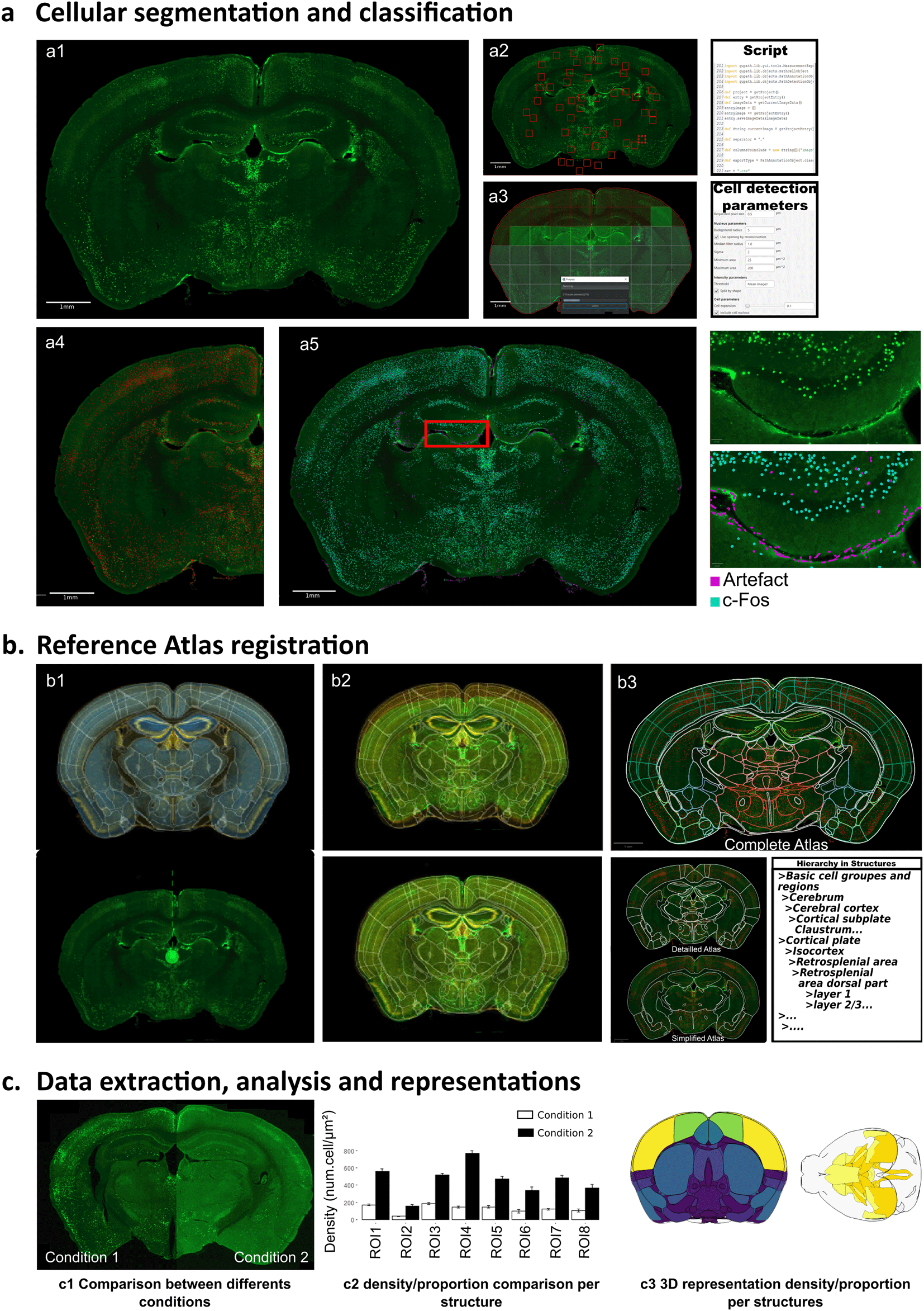
The workflow is composed of three consecutive steps: a, cellular segmentation and classification using an automated script in QuPath; b, reference atlas registration with ABBA software; and c, data extraction, analysis and representation. a) Cellular segmentation begins with c-Fos immunostaining on serial sections, which are then imaged on a slide scanner (a1). Adaptive thresholding is performed using a script that extracts values from random fields (a2), then applies it to the entire section (a3) for optimal cell detection. Once cell detection is complete (a4), a classifier is used (a5) to differentiate c-Fos positive cells (blue) from artifacts (purple), as illustrated in a higher magnification of the dentate gyrus. b) During the second step, ABBA software is used to distribute and register individual sections onto the Allen reference brain atlas (b1). Elastic algorithms are used to improve section adaptation to the reference atlas, followed by final manual refinement (b2). Different atlas resolution levels can be generated based on the hierarchical organization of the Allen mouse brain atlas (b3). c) Data analysis begins with quality control for individual mice, followed by intra- and inter-groups comparisons using a R script provided as supplementary material (c1). Different methods can be performed for comparative statistical analysis and data presentation as bar graphs (c2) or 2D/3D color-coded brain representations using BrainRender (c3).

Stage 1 - Cellular segmentation and classification (Figure 1a): This relies on QuPath¹² (https://qupath.github.io/). Scripts for automation and adaptive thresholding using Qupath or ImageJ are provided. Both result in the accurate detection of labeled cells while reducing the variability observed between sections. Classifiers used to detect and subtract artifacts were also benchmarked and included in the workflow.

Stage 2 - Reference atlas registration using ABBA (Figure 1b): This relies on ABBA (Aligning Big Brain Atlases, https://abba-documentation.readthedocs.io/). Essential principles for the optimization of the registration procedure are provided.

Stage 3 - Data extraction, analysis and representation (Figure 1c): analysis was performed in R in two steps (i.e., 1) quality control of individual animals and 2) comparison of animal groups corresponding to two independent scripts. A third script allows the representation of results in a 2D/3D model using BrainRender (https://github.com/brainglobe/brainrender,¹³).

Histology & Imaging

We aimed to develop a universally applicable methodology for comparing the results produced by different laboratories or under varying experimental conditions. To this end, we used two sections of thickness (30 and 50 micrometers), encompassing sections generated via cryostat or vibratome methods. Notably, we observed no discernible differences in the section quality or immunostaining efficacy between the two techniques. In both cases, staining was performed on free-floating sections. Thus, the workflow described below can be applied to a range of sectioning/staining procedures that are commonly used in diverse laboratory settings. However, for optimal whole-brain analysis, several rules must be strictly followed. For whole-brain estimation, it is essential to follow strict stereological rules for tissue collection. Homogeneous tissue sampling is essential for unbiased quantification (https://www.stereology.info/sampling/). Given the considerable variation in volume across brain structures, we recommend a section interval of 250 μm or less for c-Fos quantification owing to the abundance of c-Fos-positive cells. For particularly small brain structures or antigens exhibiting sparse labeling, a higher sampling rate (i.e., smaller section interval) may be necessary. In our analysis, we chose to collect one section every eight sections in paradoxical sleep (PS) and wakefulness (WF) conditions (thickness: 30 μm; section interval: 210 μm) and one section every six in social behavior (SB) condition (thickness: 50 μm; section interval: 250 μm).

We recommend using a slide scanner for imaging. Here, we employed a Zeiss Axioscan slide scanner; however, QuPath supports a wide range of file formats, making the workflow compatible with the data acquired from various slide scanners and imaging systems. The optimal acquisition parameters tailored to specific experimental conditions must be determined by the user. The settings should be balanced to avoid saturated or weak signal detection. We deliberately analyzed the raw images without correcting for excitation field inhomogeneity, thereby demonstrating the robustness of our workflow under variable imaging conditions, representative of routine experimental practice, while also highlighting its potential for even greater performance following further optimization. For thick sections, such as those used in this study, multiple focal planes should be imaged to ensure full visualization. Depending on the staining of interest, specific functions available in the Zen software (Zeiss) can be applied to improve scan sharpness, thereby facilitating quantification precision. Here, we used the wavelet function in the Zeiss Zen software, which decomposes images into different spatial scales to reduce the background signal and emphasize fine structural details. Finally, we recommend exporting single-section mosaics using the “processing-batch-split-scene” function (Zen software, Zeiss) at the end of the acquisition rather than loading the full. czi file containing multiple sections in QuPath. This practice is particularly useful when dealing with sections from multiple wells (e.g., wells 1 and 7 of a series of 12 to obtain a 1:6 sampling rate), allowing for the orderly arrangement of sections before importing them into Qupath. Indeed, the correct ordering of sections is required to facilitate registration (see Stage 2) and subsequent analysis (see Stage 3).

Stage 1: Cellular segmentation and classification using QuPath

First, we assessed the accuracy of c-Fos detection using QuPath ( Figure 2a). To this end, we manually identified immunoreactive cells in two brain regions, the piriform and anterior cingulate areas, which showed marked differences in c-Fos density and distribution ( Figure 2b, “manual”). We then selected an arbitrary threshold (low: 1000), matching the manual counts after careful visual inspection, and used this as a reference against which automated detections at other thresholds ( Figure 2b) or automatic thresholding (see below) were compared. We further defined two additional thresholds (medium: 3274 and high: 6127), corresponding to the detection of ~50% and ~30% of all c-Fos-positive cells, respectively. Visual inspection confirmed the precision of the detection process, showing an inverse correlation between the threshold level and number of detected cells ( Figure 2b). Accordingly, the average c-Fos intensity was 9328 ± 356 Gray values, with a low threshold, yielding 24067 ± 1022 c-Fos-positive cells per section. This value increased with the medium (18452 ± 585) and high thresholds (24144 ± 672), while the number of detected cells decreased (8308 ± 442 and 4746 ± 349, respectively). Thus, QuPath allows accurate detection of c-Fos+ cells with flexible adjustment of detection sensitivity to capture populations with different staining intensities.

Figure 2. Automation and refinement of c-Fos positive cell detection and classification.

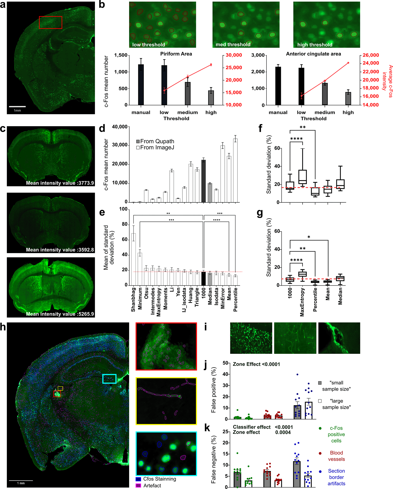
a) Represent immunostained for c-Fos. Captions illustrate how detection at 3 arbitrary threshold levels, i.e. low (1000), medium (3274) and high (6127), impacts the number of detected cells. b) Quantification of detected cell number and averaged intensities at the three arbitrary thresholds (grey level) compared to manual quantification on two different brain regions, the Piriform and Anterior cingulate areas. Data represent n = 3 brain sections per structures and threshold level. c) Illustration of pronounced staining intensity variability between subsequent sections. All our quantification analysis comparison are made using low threshold as a reference because of its similarity to manual detection. d) Quantification of c-Fos positive cells using reference thresholding (black bar, 1000) or various automatic thresholding methods in QuPath (grey bar) or ImageJ (white bars). Note the variability in detection efficiency. Data represent n = 14 brain sections per thresholding method. e) Quantification of density variability (i.e. standard deviation) between three consecutive sections using an arbitrary threshold of 1000 (black bar) or various automatic thresholding methods in QuPath (grey bar) or ImageJ (white bars). Data represent n = 14 brain sections per thresholding method. f-g) Selection of automatic thresholding methods based on detection efficiency and reduced count variability (shown in d and e) for complementary analysis of performance with consecutive sections showing heterogeneous (f) and homogeneous (g) staining. Standard deviation of counts obtained from section triplicates are shown The “Percentile”, “mean” and “median” methods can be used for automatic thresholding, offering various detection sensitivities and similar or reduced count variability compared to manual arbitrary thresholding (red line, 1000). Data represents n=38 sections per thresholding method. h) Representative section showing the main sources of artifacts (purple) to distinguish from positive cells signal (blue), i.e. mainly border effects (see red box) and blood vessels (see yellow box). i-k). Comparison of two “training” methods for distinguishing artifacts from positive cells using classifiers (i.e. “large sample size” and “small sample size”, see methods). Manual validation of classification errors in identifying positive cells (j) or artifacts (k) in regions with a large number of cells or artifacts (i). Data represent n = 12 samples per classifier analyzed and region analyzed. Note that both methods show comparable efficiency in accurately detecting positive cells, but the “large sample size” training method significantly reduces errors while detecting artifacts. Data are expressed as Mean ± SEM. * P < 0.05; ** P < 0.01; *** P < 0.001.

Quantitative analysis of c-Fos immunodetection faces two primary challenges that impact accuracy: 1) variability of staining intensity within sections and 2) variability of staining intensity across sections induced by the immunostaining method used (floating sections, see material and methods). Although manual adjustment of the detection thresholds, as demonstrated earlier, can mitigate these challenges, unbiased methods are preferable. While the first source of variability may carry biological significance, the second is largely experiment-dependent, resulting, for example, from tissue folding or adherence to vessel walls during staining. QuPath only offers limited capabilities for adaptive thresholding but mostly relies on experimentator-defined values. Therefore, we explored different means of performing automatic thresholding ( Figure 2c-e). We evaluated and compared the following approaches: 1) Internal automatic thresholding (QP): which relies on the automatic detection of the median intensity measured within individual sections. A script (“Automatic_ threshold_application_(Qupath)”) facilitates the extraction of this variable to define the threshold for cell detection in each section. 2) External automatic thresholding (IJ): This approach relies on thresholding methods implemented in ImageJ. A script (“Automatic_threshold_application_(ImageJ)”) was used to define random fields to determine the average staining intensity per section. Because auto-thresholding can be influenced by local variations in c-Fos density, we designed our approach to calculate thresholds from either the entire section or up to 50 randomly selected regions. This strategy minimized the confounding effects of locally high c-Fos-positive cell density.

To determine the best automatic thresholding methods, we compared the results obtained on adjacent sections showing variable staining intensities using an arbitrary threshold of 1000 (22073 ± 1414 detections per section) to those obtained through 16 automatic thresholding methods ( Figure 2d-e). The mean number of detections per section and density standard deviation between adjacent sections (triplicate) were measured. Results highlight that thresholding methods result in varying levels of detection ( Figure 2d), ranging from a 48,88% increase (Percentile, 32863 ± 2045 detections) to a 99% decrease (Shangbag, 135 ± 27 detections) compared to arbitrary thresholding “1000.” Several methods have yielded detection counts comparable to those obtained with an arbitrary threshold, such as the “Huang” method (19931 ± 1371 detections). Among all tested methods, the “Mean” (23988 ± 1641 detections), “Median” (10087 ± 600 detections) and “MaxEntropy” (2531 ± 239 detections) were of interest, as these approaches enabled detecting a range of c-Fos intensities close to the low, medium and high thresholds tested above. We next checked how different threshold methods influenced the variability in cell counts between three consecutive sections, taking as a reference the arbitrary thresholding “1000” ( Figure 2e). Statistical analysis of the standard deviation revealed a significant influence of the thresholding methods on cell counts (F(2,336;30.37)=17.90; P<0.0001; Greenhouse–Geisser ε = 0.1460). We observed that specific automatic threshold methods resulted in increased variability in cell counts compared to the arbitrary thresholding “1000,” notably “Shanbhag” (+300%, P<0.01, Dunnett’s multiple comparison test). In contrast, “Mean” and “Percentile” decreased this variability (P<0.01, -20% for Mean and -30% for Percentile) while “MaxEntropy” and “Median” demonstrated no significant effect. To complement these findings, we selected 4 automatic thresholding methods (“MaxEntropy,” “Percentile,” “Mean” and “Median”) and evaluated in more detail the percentage of variability of cell detection on three consecutive sections showing heterogeneous ( Figure 2f) and homogenous ( Figure 2g) cell counts when using an arbitrary threshold of 1000. In heterogeneous sections ( Figure 2f), we found a similar percentage of standard deviation (SD) for “Mean” (14.39 ± 0.79%, P=0.16) and “Median” methods (21.26 ± 1.24%, P=0.42) compared to arbitrary thresholding (18.09 ± 0.94%). However, we found a lower percentage of SD with the “Percentile” method (12.32 ± 0.84, P<0.01, -31%) and higher with the “MaxEntropy” method (28.02 ± 1.577, P<0.01). In homogeneous sections ( Figure 2g), we found a similar standard deviation for “Median” methods (7.90 ± 0.50%, P=0.56) and the arbitrary threshold of 1000 (6.64 ± 0.45). The “Percentile” (3.84 ± 0.27%, P<0.01) and “Mean” (4.27 ± 0.27%, P<0.05) methods reduced standard deviation values, while “MaxEntropy” increased it (12.19 ± 0.56%, P<0.01, +50% compared to arbitrary threshold). However, despite “percentile” yielding satisfactory outcomes in terms of the number of identified cells and standard deviation, it was discarded due to visual inspection revealing over segmentation, with many artifacts taken into account. Altogether, these results led to the selection of the “mean” (MeanIJ), “median” (MedQP) and “MaxEntropy” (MaxE) methods, based on their capacity to reveal varying levels of detection without exacerbating or even reducing the variability of cell counts.

Cell counting often results in false positive detection, which can arise from blood vessel autofluorescence or antibody aggregation at section borders ( Figure 2h-i). Such artifacts can be readily recognized by an experimenter (e.g., linear arrangements of oval-shaped nuclei corresponding to blood cells or large nonspecific staining patches) but must be excluded from automatic detection. To address this issue, classifiers using machine learning approaches integrated within QuPath (called “cell classifier”) can be used to detect artifactual detection. The machine-learning classifier in QuPath does not independently generate a global intensity threshold. Instead, the initial thresholding step serves only to identify candidate objects (cells) based on signal intensity, ensuring that the classifier is applied to plausible detections rather than to all image pixels. The Random Trees Classifier is then trained on these candidates using multiple features (intensity, morphology, texture) and user-provided labels (‘positive’ vs. ‘artifact’). In this way, thresholding provides a consistent entry point, whereas the classifier refines the decision by integrating additional features beyond the intensity. Thus, the classifier does not replace thresholding but builds upon it, yielding a more accurate discrimination of true positive cells. However, the efficiency of a classifier relies on the training conducted by the experimenter, which makes it challenging to determine the optimal level. Thus, while undertraining may not be sufficient for the optimal classification of artificial signals, overtraining may result in ambiguous results. We assessed two strategies for classifier training. The first strategy, termed “Small sample size”, involves sampling small areas with few detected cells (<10) and repeated numerous times (>90 repeats per detected cell class). Conversely, the second strategy, termed “large sample size,” consists of sampling larger areas with a higher number of detected cells (>50) but fewer repetitions (<10 repeats per detected cell class). To compare both strategies, we manually curated the results obtained using each approach to quantify the number of falsely classified cells as “positive” or “artifact” across three distinct areas containing c-Fos-positive cells, blood vessels, and section border artifacts (n=12 sections per area and classifier across four mice). Results indicate that no changes were noted in the proportion of cells falsely classified as positive ( Figure 2j; F(1,66) = 0.1941, P = 0.6610). However, the “large sample size” strategy resulted in a significant reduction of cells falsely classified as artifacts ( Figure 2k, F(1,66) = 38.32, P < 0.0001). Altogether, our results underscore the superiority of the “large sample size” strategy, which was therefore used in subsequent analyses.

Stage 2- Reference atlas registration using ABBA

Several atlases have been made available online. The open-access Allen Brain Atlas quickly established itself as a reference for most neuroanatomists (http://atlas.brain-map.org¹⁴). Following cell detection and classification, sections were aligned to this reference atlas using the Aligning Big Brain Atlases (ABBA). The registration workflow implemented in this software is detailed online (https://abba-documentation.readthedocs.io/). It facilitates the adaptation of reference brain atlas contours to sections through a combination of automatic (i.e., elastix affine + spline registration) and manual algorithms (BigWarp¹⁵), ensuring that deformations are applied solely to the contours, leaving the brain section image and detecting cell geometry unaltered. The registration workflow consisted of several steps that were evaluated to establish the most efficient approach. The initial step involved identifying key sections for optimal rostrocaudal positioning and cutting plane correction. At the beginning of the alignment process, we recommend selecting the most rostral and caudal sections. The initial rostrocaudal registration can be achieved using the maximal section interval offered by the reference atlas. Subsequently, the section interval can be reduced to fine-tune section placement. If the sampling is uniform, the sections can then be evenly distributed between the two key sections. Validation was then performed by visual inspection of all sections to rectify any potential errors that may have occurred during sectioning (i.e., missing or duplicated sections). ABBA registration further facilitates correction for section inclination along the “x” and “y” axes. Indeed, even if brain sectioning protocols are standardized using brain casts,¹⁶ variations across the brain are common. For precise cutting-plane correction, we recommend the following workflow and landmarks: The “x” axis correction is done by focusing on a caudal section corresponding to section 79-80 of the Allen adult mouse atlas (Extended Data Figure 1a). This section, with a well-defined dorsal hippocampus and the separation of the corpus callosum into two hemispheric structures, is prone to notable “x” axis changes. Positive inclination accelerates the rostrocaudal separation of the corpus callosum, whereas it persists as a continuous structure on a larger number of sections with negative inclination. The dorsal hippocampus within this section can be used for optimal “y” axis correction, as even a slight inclination in the “y” axis results in well visible differences between the two hippocampi, particularly evident for the dentate gyri (Extended Data Figure 1a). Validation of “y” axis correction can then be conducted by selecting a more rostral section (section 53 of the Allen adult mouse atlas, Extended Data Figure 1b), where the anterior commissure is continuous between hemispheres, thereby confirming “y” axis correction.

Following the establishment of initial parameters, it is recommended to sequentially employ both linear (affine) and nonlinear (spline) “elastix algorithms” integrated into the ABBA software to further refine the section registration. This process involves selecting a specific channel of the image (e.g. DAPI, c-Fos … Figure 3a) to align it with one of the reference atlases available in ABBA (i.e. Nissl or 3D model “Ara”, Figure 3b). To systematically evaluate the efficacy of registration across all channels and reference atlases, we adopted the following approach. We first confirmed the improvement in registration accuracy through the application of affine (applied once or twice) and spline transformations using the c-Fos channel and Nissl Atlas. We then compared the results obtained using distinct staining channels (including counterstaining for neurons, i.e., NeuN and myelin, i.e., MBP). Finally, we compared the results obtained using the most effective channels with both Nissl and “Ara” Atlas models. For quantitative assessment, user-drawn contours of selected regions were systematically compared with the results achieved by the registration process (n = 8 regions of interest analyzed per combination of parameters evaluated). This comparison allows for the calculation of a Dice coefficient, whose value increases with the contour superposition. A Dice coefficient greater than 0.7 indicates acceptable contour superposition.¹⁷

Figure 3. Optimization and validation of atlas registration.

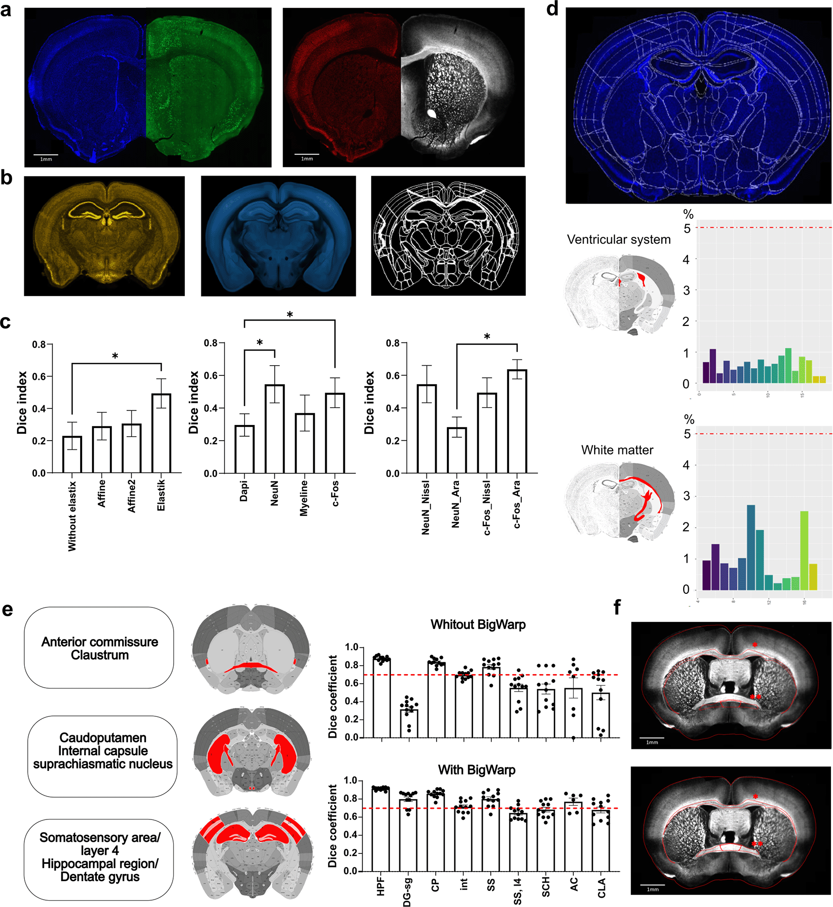
a) Channel tested for atlas registration: DAPI (blue), c-Fos (green), NeuN (red) and MBP (white). b) ABBA atlases tested for atlas registration: Nissl Atlas (brown), Ara Atlas (“3D model”, cyan) and Atlas only composed by brain regions contours. c) Comparison of atlas registration accuracy using various channels and/or atlases. Dice correlation for white matter area (n = 8) show conditions for which best results are obtained. The first bar graph illustrates the effect of each elastix algorithm (Affine and Spline) on registration obtained with the c-Fos channel and the Nissl atlas. Note that Affine and Spline should both be applied for best results, while repeating Affine does not improve accuracy. The second bar graph evaluates the impact of channel selection on registration accuracy using the Nissl Atlas. The final graph shows the impact of choosing different atlases while using the two best channels, i.e. NeuN or c-Fos to perform the registration. d) Regions used (red) for quality control of section registration based on c-Fos detection in regions devoided of neuronal cell bodies, i.e. white matter (WM) and ventricular system (VS). A score higher than 5% indicates misregistration. e) Automatic registration validation by comparison with ROI defined by anatomists. (n = 12 per structure). Dice index above 0.7 is considered as good overlap. While registration is optimal for large regions, small and/or tortious regions (i.e. dentate gyrus) necessitate manual refinement using BigWarp. Abbreviations: HPF, hippocampal formation; DG-sg, Dentate gyrus, granule cell layer; CP, caudoputamen; int, internal capsule; SS, somatosensory areas; SS,l4, layer 4 of somatosensory areas, SCH, suprachiasmatic nucleus; AC, anterior commissure; CLA, claustrum. f ) Illustration of registration parameters combination leading to lowest (above, c-Fos_affine_nissl) and highest (below, c-Fos_spline_Ara) Dice index. Red ROI correspond to brain region registration after parameters application (*: Corpus callosum; **: Anterior commissure). Data are expressed as Mean ± SEM, * P < 0.05.

Results confirmed the efficiency of sequentially applying linear and nonlinear “elastix algorithms” (P = 0.01, Friedman test) to significantly improve registration accuracy, as evidenced by the Dice coefficient increasing from 0.23 ± 0.08 without anything to 0.49 ± 0.09 when elastix registrations were applied (P < 0.05). Our quantification also revealed that the repetition of affine registration did not yield further improvement in the Dice coefficient (P > 0.99, Figure 3c). Further, channel selection also significantly improved registration accuracy (P < 0.01, One-way Anova) with a significant Dice coefficient improvement when NeuN and c-Fos channels are used compared to DAPI counterstaining (0.55 ± 0.11 and 0.49 ± 0.09 respectively for NeuN(P = 0.0117) and c-Fos(P = 0.0402) vs. DAPI 0.30 ± 0.07). Interestingly, MBP counterstaining showed no benefits in terms of registration accuracy. Finally, we aimed to test the reference atlases available in ABBA. Results revealed a more limited impact of the reference atlas selection (P = 0.05, Friedman test), with the 3D model ‘Ara’ resulting in higher registration accuracy using c-Fos channel than NeuN (0.64 ± 0.06 c-Fos_Ara vs 0.28 ± 0.06 NeuN_Ara, P = 0.04). Furthermore, the Dice index obtained with NeuN_Nissl and c-Fos_Nissl showed no significant difference with c-Fos_Ara (both P > 0.99), providing a certain degree of flexibility for users in atlas selection. Taken together, these findings underscore the importance of selecting the appropriate image channel, reference atlas, and registration procedure to achieve the highest Dice coefficient consistently. They further revealed that DAPI counterstaining is inadequate for optimal registration, while myelin counterstaining impedes this process. Based on these results, we adopted the elastix transformation (Affine + Spline) in conjunction with the c-Fos channel and 3D model ‘Ara’ atlas for precise section registration in the following analysis.

To systematically validate the accuracy of cell detection and registration and facilitate the identification of aberrant sections, we implemented a quality control step within our workflow. We provide a script (“QuPath_ABBA analysis_QualityControl.R”) that should be used in all sections before proceeding with further analysis. This script can be run on a list of “csv” files contained within a folder to automatically generate a figure composed of six panels that provide distinct types of information to the experimenter (see Extended Data Figure 2). Aberrant numbers should prompt careful consideration of sections, that is, acquiring new images, excluding them from quantification, or conducting refined analyses. Panels a and b (i.e., Num.c-Fos/slices and density of c-Fos/slices) facilitate the identification of missing or aberrant sections (e.g., folded or broken sections, out-of-focus sections). Panel c (i.e., Percentage artifact/slice) highlights sections presenting aberrant ratios of detected artifacts among the total number of detected cells in all sections. Significant fluctuations in this metric indicate sections containing artifacts such as dust. Panels d and e (i.e., percentage of c-Fos in two control regions, i.e., the ventricular system and the white matter (composed of the corpus callosum, body, anterior forceps and olfactory limb, the internal capsule, allowing to cover the entire rostro-caudal extent of the brain) provide important information on registration accuracy due to the absence of c-Fos-positive cells ( Figure 3d). An arbitrary “red line” appeared at 5%, corresponding to 5% of the detected cells present in the control regions. This value is arbitrary (in our hand, values exceeding 3% are extremely rare) and can be lowered by the experimenter to increase stringency when high accuracy is required; for example, when only small differences are expected between experimental groups. Sections above this line should receive immediate attention for improving registration by repeating the aforementioned steps or performing manual adjustments using the BigWarp registration refinement step for registration accuracy improvement, as detailed below. Finally, Panel f (i.e. density of c-Fos in main brain regions) allows rapid verification of whether all main, non-overlapping brain regions are faithfully represented within the dataset ( Figure 3e).

We recommend using BigWarp with caution, as excessive use or application to damaged or incomplete sections may introduce local deformations. However, we devised a workflow that significantly enhanced the registration efficiency, particularly for small or intricately shaped brain regions ( Figure 3f). For optimal results, we recommend the following steps: 1) realigning section borders when necessary, 2) realigning interhemispheric “midline,” 3) realigning white matter tracts, and 4) realigning elongated, sinuous brain regions, such as the dentate gyrus. We validated this workflow by calculating Dice coefficients for nine brain regions manually delineated by three anatomists and comparing registrations before and after applying BigWarp. We selected ROIs of different sizes in both the dorsal and ventral areas of the rostral and caudal sections, that is, the hippocampal formation, dentate gyrus (granular layer), caudoputamen, internal capsule, somatosensory cortex, layer 4 of the somatosensory cortex, suprachiasmatic nucleus, anterior commissure, and claustrum. Data revealed that Dice coefficient exceeds 0.7 for most medium to large anatomical regions, i.e. somatosensory area (0.80 ± 0.02), caudoputamen (0.86 ± 0.01), hippocampal region (0.91 ± 0.005), with minimal impact from “BigWarp” adjustments. However, registration accuracy for the smallest or more convoluted structures may vary, requiring systematic BigWarp manual adjustment to reach a Dice coefficient equal or exceeding 0.7, e.g., anterior commissure (0.77 ± 0.04, +40% compared to prior-BigWarp), internal capsule (0,71 ± 0,02, +2%), suprachiasmatic nuclei (0.68 ± 0.03, +26%). Together, these results underscore the importance of employing BigWarp to achieve optimal registration of small or intricate brain regions and offer a means to validate registration accuracy.

Stage 3- Data extraction, analysis and representation:

We refined a selection of brain regions, i.e. “major divisions,” “summary structures,” “full list” that correspond to distinct hierarchical levels of the 3D Allen Mouse Brain Common Coordinate Framework (CCFv3;¹⁸ 9, 206 and 467 regions, respectively, Figure 4a). We manually curated these atlases at different resolutions to minimize the overlap between brain regions and to avoid any gaps within representations. This is important not only for having a faithful representation of the entire brain at different resolutions, but also to avoid any artifacts when representing results. These atlases facilitate the optimal representation of the acquired results from BrainRender, a Python library for the visualization of three-dimensional neuroanatomical data (https://github.com/brainglobe/brainrender). For each region of the selected atlas, the “QuPath_ABBA analysis_Comparison groups. R” script extracts c-Fos cell count, the surface of areas, and calculates the density or proportion of c-Fos-positive cells per condition. The 3D data representation script will then represent c-Fos cell densities within a given condition and/or compare cell densities or proportions between the two conditions. Finally, a list of regions exhibiting significant changes between the conditions can be generated. A 3D representation of obtained results can be generated with BrainRender, using the “3D data representation” script (see Extended Data Figure 3).

Figure 4. Detection restricted to brighter c-Fos positive cells reduces results relevance.

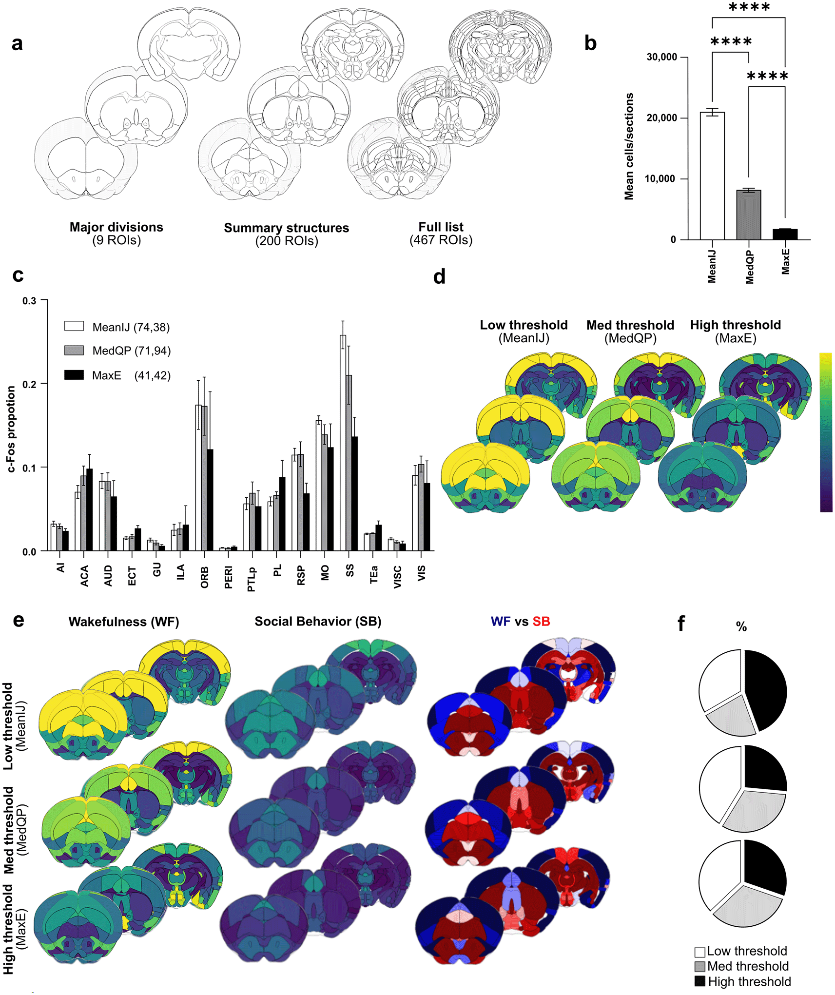
a) Illustration of three atlases for whole brain c-Fos analysis at different resolutions. b) Automatic thresholding using low (MeanIJ), med (MedQP) and high (MaxE), allows detecting various numbers of cells. c) Automatic thresholding methods enable comparison of the proportion of c-Fos positive cells in various brain regions (N = 5 mice), here areas composing the isocortex. Note the reduced contrast observed between cortical regions when using higher thresholds, as indicated by values from non-parametric one-way Anova (Krustal-Wallis) statistics showing reduced dispersion of c-Fos proportions. d) Corresponding representations of c-Fos cell density at selected rostro-caudal axis coordinates. Note the loss of contrast when using high thresholding methods. e) Comparison of c-Fos cell density using “summary structures atlas” in mice (N = 5 mice per condition) exposed to two different behavioral paradigms, i.e. Wakefulness (WF) and Social Behavior (SB). A direct comparison highlights region preferentially activated in WF (blue gradient) or SB (red gradient) conditions. f ) Percentage of regions previously identified as active in social interactions and showing significantly higher activity in SB condition when using Low, Med and High automatic thresholding. Results are shown for “major division” (top), “Summary structures” (middle) and “Full list” (bottom) atlases. Note that high thresholding identifies a lower percentage of relevant regions. Abbreviations: AI, Agranular insular area; ACA, Anterior Cingulate Area; AUD, Audritoy Areas; ECT, Ectorhinal Area; GU, Gustatory Areas; ILA, Infralimbic Area; ORB, Orbital Area; PERI, Perihinal Area; PTLp, Posterior Partietal Association areas; PL, Prelimbic area; RSP, Restrosplenial area; MO, Somatomotor areas; SS, Somatosensory areas; Tea, Temporal Association areas; VISC, Visceral area; VIS, Visual areas. Data are expressed as Mean ± SEM. **** P < 0.0001.

Having benchmarked various automatic thresholding methods that allow unbiased detection of either a large number of cells or a subset (i.e., brighter cells), we sought to determine the most informative approach for studying brain-wide activity patterns with c-Fos. To this end we selected three levels of c-Fos positive cell detection ( Figure 4b) and applied them to mice subjected to the “wakefulness” (i.e. WF) paradigm, resulting in different detection levels: MeanIJ, defined as low threshold, (21046 ± 632 cells/sections); MedQP, defined as med threshold, (8184 ± 334 cells/sections, i.e. 39% of meanIJ), and MaxE, defined as high threshold (1743 ± 90 cells/sections, i.e. 8% of meanIJ). Analysis using the “summary structure” atlas revealed that a higher threshold led to reduced contrast in cell proportions observed in different brain regions, as illustrated for cortical areas ( Figure 4c). For instance, while most c-Fos cells were detected within the somatosensory cortex of “wakefulness” mice with low and medium thresholding methods, this pronounced enrichment was lost when brighter cells were detected (0.26 ± 0.02 MeanIJ vs. 0.14 ± 0.02 MaxE P < 0.01). This reduced amplitude of observed differences between cortical areas was supported by a higher K value when using a low threshold (MeanIJ, 74.38; Krustal Wallis), which gradually decreased with higher thresholding values (MedQP, 71.94 and MaxE, 41.42). Furthermore, the 3D visualization of c-Fos cell density obtained at the three thresholds clearly highlighted the gradual loss of contrast observed between the brain regions ( Figure 4d). Thus, whereas comparison of low (MeanIJ) and medium threshold (MedQP) detection led to 94.5% similarities of all ROIs being detected as significantly different, this number decreased to 32% when a higher threshold (MaxE) was applied, further supporting a profound reduction in contrast when only brighter c-Fos cells were detected. Noticeably, this effect appeared to be more pronounced within the cortex, as the contrast in cell proportion within subcortical structures remained less affected by the methodology used for cell detection (see Extended Data Figure 4).

To further analyze the consequences of this reduced contrast for comparisons between different experimental groups, we compared c-Fos positive cell densities in mice subjected to “wakefulness” and “social behavior” paradigms (WF and SB, respectively), using the three thresholding methods outlined above. To visually inspect the obtained results, we used a color code highlighting the differences between conditions, that is, a blue gradient associated with regions activated in WF and a red gradient associated with those activated in SB ( Figure 4e). Regions showing significantly higher levels of activity in “social behavior” were listed at all hierarchical atlas levels (“major divisions”, “summary structures”, “full list”) and compared to those previously identified in a classical study,¹⁹ ( Figure 4f). While both MeanIJ and MedQP thresholding consistently yielded comparable outcomes in identifying regions previously identified as activated during social behavior, the results obtained with MaxE were more mitigated.

In summary, our careful benchmarking underscores the importance of integrating all pre-established optimal parameters for thorough whole-brain analysis. Specifically, we recommend using MeanIJ or MedQP thresholding methods alongside a “large sample size” classifier refinement to ensure the accurate detection of condition-specific neuronal activity patterns. Furthermore, for ABBA atlas registration, we recommend implementing elastix registration using c-Fos/NeuN markers in combination with Ara or Nissl atlases, followed by refinement using BigWarp registration for optimal results.

Identification of distinct activity patterns in different behaviors and at different scales

We began by validating our workflow by comparing c-Fos expression patterns in groups of mice (N = 5) subjected to distinct behavioral paradigms: wakefulness (WF), social behavior (SB), and paradoxical sleep (PS). Analysis of c-Fos-positive cell densities within each group revealed distinct activity patterns under the three conditions ( Figure 5a). For example, activity in somatosensory and motor cortical areas was prevalent in WF, whereas activity in frontal cortical areas and periventricular regions was more pronounced in SB and PS, respectively ( Figure 5a). However, these differences were accompanied by pronounced differences in activity levels between the groups, with the number of c-Fos-positive cells being significantly lower in PS than in WF or SB (Extended Data Figure 5a-b). This discrepancy prompted us to investigate whether such substantial differences in activity hinder the detection of condition-specific patterns of c-Fos expression. To address this, we first compared the results obtained by quantifying the raw cell numbers and cell densities within the cortex (Extended Data Figure 5c, d & 6a, b). As anticipated, a comparison of SB or PS with WF revealed pronounced effects of activity level on the outcomes. For instance, all cortical regions appeared to be significantly lower in PS/SB than in WF, reflecting a global decrease in activity while impeding the identification of condition-specific cortical activity patterns.

Figure 5. Spatial analysis of activity patterns in different behaviors and at different scales.

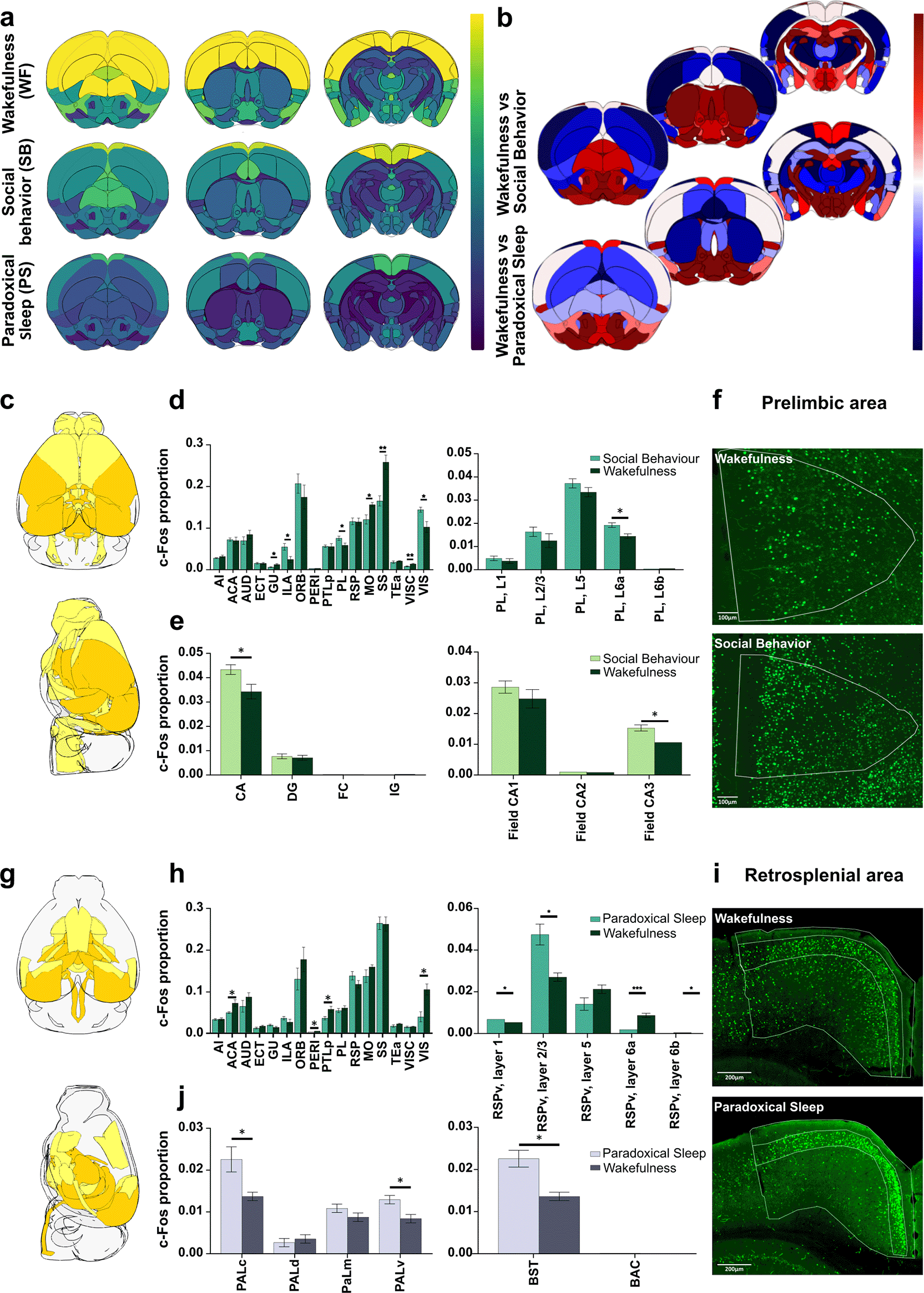
c-Fos expression patterns related to different behaviors can be visualized and explored using several qualitative and quantitative representations. a) 3D projections of c-Fos density in various brain regions (“Summary structure” atlas). b) Direct comparison highlighting regions preferentially activated in WF (control condition, blue gradient), when compared to SB or PS (red gradient, upper and lower sections respectively). c-i) Quantitative data analysis can be visualized by two methods. First, by identification of brain regions showing significant differences in c-Fos proportions on a 3D model, i.e. here for Isocortex areas (c, g, light yellow = P < 0.05; dark yellow = P < 0.01). Second, by using bar graphs for defined brain regions at different resolutions (“summary structures”, left, “full list”, right)). Analysis of the Isocortex (d, h) shows different patterns of c-Fos expression following SB and PS. Focus on specific isocortical areas, i.e. prelimbic area (d) or retrosplenial area (h) highlight more discrete differences. f, i) Corresponding immunostainings illustrating global (f) or layer specific (i) c-Fos induction. e, j) Analysis of the hippocampal formation and pallidum at similar increasing resolution (i.e ammon’s horn and pallidum medial/caudal region, respectively) highlight significant differences in c-Fos expression pattern in SB (e) and PS (j) conditions. Abbreviations: AI, Agranular insular area; ACA, Anterior Cingulate Area; AUD, Auditory Areas; ECT, Ectorhinal Area; GU, Gustatory Areas; ILA, Infralimbic Area; ORB, Orbital Area; PERI, Perirhinal Area; PTLp, Posterior Parietal Association areas; PL, Prelimbic area; RSP, Restrosplenial area; MO, Somatomotor areas; SS, Somatosensory areas; Tea, Temporal Association areas; VISC, Visceral area; VIS, Visual areas; CA, Ammon's horn; DG, dentate gyrus; FC, Fasciola cinerea; IG, Induseum griseum; PAL, Pallidum (d: dorsal, c: caudal, m: medial, v: ventral); BST, Bed nucleus of stria terminalis; BAC, Bed nucleus of the anterior commissure. Data are expressed as Mean ± SEM, *P < 0.05; **P < 0.01; ***P < 0.001. (N = 5 mice/condition).

To facilitate the extraction of these nuanced changes in c-Fos expression patterns between conditions, we devised a method to calculate the proportion of c-Fos-positive cells per brain region by normalizing cell counts to the total number of cells detected per section. For a qualitative visual representation of the obtained results, we used a color gradient highlighting differences between conditions, that is, a blue gradient indicating regions activated in WF and a red gradient indicating those activated during SB or PS ( Figure 5b, Extended Data Figure 5e). We complemented these visual representations using more quantitative analyses that can be automatically performed at different scales. To this end, we incorporated the calculation of P-values between conditions in our script, allowing their representation on 3D brain models (yellow = P < 0.05, orange = P < 0.01, Figure 5c-g, Extended Data Figure 6c), along with bar graphs ( Figure 5d-e, h-j). Notably, this analysis can be performed at different resolutions by simply selecting appropriate atlases.

To illustrate the versatility of this approach, we compared the c-Fos labeling patterns within cortical areas between WF and SB ( Figure 5d-f) or WF and PS mice ( Figure 5h-j), which we complemented by performing a more detailed analysis of cortical layers in select areas. Using this multiscale approach, our results revealed significantly increased c-Fos expression is SB compared to WF mice in the infralimbic cortex (0.025 ± 0.007 for WF and 0.055 ± 0.008 for SB; P = 0.03) and prelimbic cortex (0.060 ± 0.005 for WF and 0.075 ± 0.007 for SB; P < 0.05), whereas other regions, such as the retrosplenial area, showed no significant changes ( Figure 5d). Focusing on the prelimbic area, our results refined these initial observations by highlighting that the observed increase in c-Fos expression was primarily localized within layer 6a ( Figure 5d). Similarly, our results showed an increased c-Fos proportion within the Ammon’s horn of the hippocampal formation in SB mice (0.034 ± 0.003 for WF and 0.043 ± 0.002 for SB; P = 0.04), which analysis at higher resolution was specific to the CA3 fields (CA3:0.010 ± 0.000 for WF and 0.015 ± 0.001 for SB; P = 0.02, Figure 5e). Finally, while we found a higher proportion of c-Fos during PS in the caudal and ventral pallidum, analysis at higher resolution refined these observations by showing the involvement of the bed nucleus of the stria terminalis (0.022 ± 0.002 for PS and 0.014 ± 0.001 for WF, P = 0.02, Figure 5j). Such a multiscale analysis also enabled the identification of layer-specific changes in c-Fos expression patterns, which were not evident when considering the cortical area as a whole. For instance, while no significant difference in c-Fos proportion was noted within the retrosplenial area when comparing WF and PS mice ( Figure 5h), a more detailed analysis highlighted a redistribution of c-Fos expression in layers 2/3 during PS (0.027 ± 0.002 for WF and 0.047 ± 0.005 for PS; P = 0.02 for ventral part; see also immunostainings in Figure 5i).

Altogether, these results underscore the relevance of comparing the raw numbers or density of c-Fos-positive cells to reveal changes in behavior-related activity levels, whereas the calculation of c-Fos cell proportions enables the identification of nuanced changes in activity patterns. Furthermore, our results emphasize the importance of conducting analyses at various anatomical resolutions, a principle that was fully implemented within the provided scripts.

Application of the automated workflow to compare activity induced by distinct behaviors in the TRAP2 mice

While previous analyses were performed in distinct animal groups, transgenic TRAP2 mice allow the comparison of behaviorally induced activity patterns within the same animal.^20,21 These mice express an inducible CRE-recombinase driven by the c-Fos promoter, leading to permanent expression of tdTomato upon administration of 4-hydroxytamoxifen (4-OHT) ( Figure 6a). Consequently, this transgenic mouse model enables the comparison of activity patterns elicited by different behaviors within individual animals. Here, we initially subjected transgenic TRAP2 mice to a wake procedure 120 min prior to 4-OHT injection. Subsequently, the same animals were exposed a week later to PS deprivation and rebound and were sacrificed 120 min later for c-Fos immunodetection ( Figure 6b).

Figure 6. Temporal Analysis of Activity Patterns Using TRAP2 Mice.

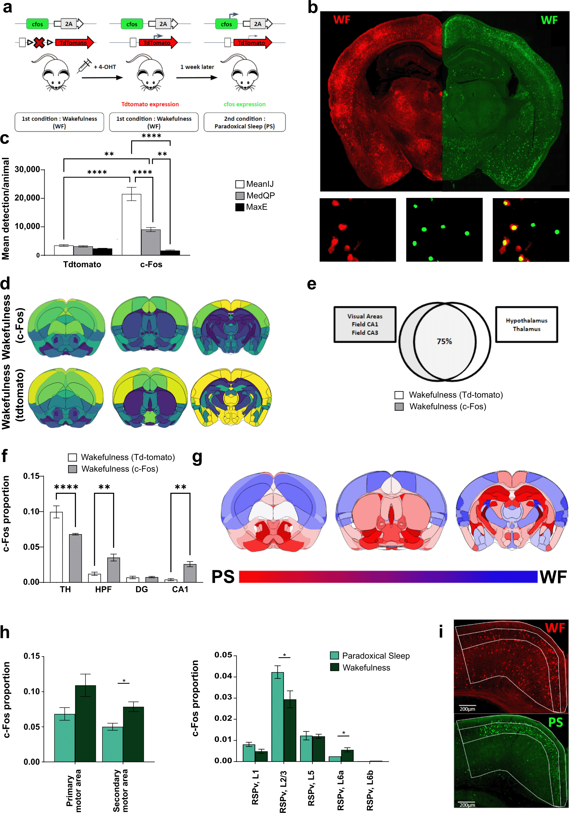
a) Workflow for experiments with TRAP2 mice. 4-OHT (80 mg/Kg, i.p.) was injected 120 minutes following a wakefulness (WF) task to induced c-Fos-driven tdTomato expression (red signal). One week later, mice were exposed to paradoxical sleep (PS) and perfused 120 minutes later for c-Fos immunodetection (green signal). b) Illustrative hemisections showing tdTomato expression and c-Fos immunodetection. c) Quantification of mean number of detections per animal using low (MeanIJ), med (MedQP) and high (MaxE) thresholding methods for tdTomato-positive cells and c-Fos-positive cells. d) 3D projections of c-Fos and tdTomato density in wakefulness. e) Diagram representing the percentage of similarity observed in c-Fos and tdTomato pattern of expression in wakefulness. While most (i.e. 75%) activated regions are common between both models, some are significantly more activated following c-Fos immunodetection (gray box) or tdTomato induction (white box). f) Proportion of tdTomato and c-Fos immunodetection in various subcortical structures. g) Quantitative 3D projections of results obtained with tdTomato mice, when comparing wakefulness (WF) vs. paradoxical sleep (PS)-induced activity (blue and red gradients represent structures activated during WF and PS, respectively). h) Comparison of Somatomotor and Retrosplenial Area (RSP) activity on PS/WF conditions. i) c-Fos/tdTomato immunostaining comparing RSP sub-structures activity on WF (tdTomato, red) and PS (c-Fos, green). (N = 4 mice per condition). Abbreviations: RSPv, retrosplenial area, ventral part; HPF, Hippocampal formation; DG, Dentate gyrus; TH, Thalamus. Data are expressed as Mean ± SEM, *P < 0.05; **P < 0.01; ***P < 0.001; ****P < 0.0001.

We first compared the number of tdTomato-positive cells detected using our three automatic thresholding methods. In contrast to the results obtained for c-Fos immunostaining (i.e., MeanIJ, MedQP, MaxE; Figure 6c), only limited differences were observed in the number of detected tdTomato-positive cells, illustrating homogeneous reporter gene expression. Consequently, the ratio of c-Fos-positive cells detected by immunostaining vs. tdTomato expression varied significantly when using various automatic thresholding methods. For instance, tdTomato-positive cells represented approximately 1/6th of the number of detected c-Fos-immunoreactive cells when using MeanIJ thresholding methods, ~1/3rd for MedianQP, and an equal number for MaxE thresholding method ( Figure 6c).

We proceeded to compare the distribution of positive cells induced by wakefulness using c-Fos immunostaining or tdTomato staining. Visualization of cell density on a 3D model using the “Summary Structures Atlas” revealed a largely similar pattern of activity between c-Fos and tdTomato detection. However, closer inspection revealed a higher density of tdTomato+ cells in the diencephalon when compared to c-Fos immunostaining ( Figure 6d), suggesting a higher expression of cFos and therefore a higher expression of CreERT2, resulting in tdTomato induction in subcortical areas. A direct comparison of cell distribution between the two groups of mice ( Figure 6e) confirmed that 75% of the regions exhibited similar activity levels. For the remaining 25%, most regions showing higher activity following c-Fos immunostaining were related to the isocortex, that is, visual areas and Field CA1/CA3 (i.e., 0.070 ± 0.013 for tdTomato vs. 0.126 ± 0.017 for c-Fos immunodetection, P < 0.001). Conversely, regions with higher activity in tdTomato mice were primarily related to the thalamus and hypothalamus (i.e. 0.09 ± 0.08 for tdTomato vs 0.06 ± 0.004 for WF c-Fos on Hypothalamus, P < 0.01, unpaired T-test). These observations were further supported by comparing the cell density within the thalamus, hippocampal formation, dentate gyrus, and CA1 subregions in both groups of mice ( Figure 6f). Comparison of positive cell proportions revealed higher activity in the thalamus using tdTomato detection (i.e. 0.10 ± 0.008 for tdTomato vs 0.07 ± 0.001 for c-Fos, P < 0.01), while higher activity was observed within the hippocampal formation and CA1 when using c-Fos immunodetection (i.e., 0.004 ± 0.001 for tdTomato vs 0.0259 ± 0.004 for c-Fos in CA1, P < 0.01). Thus, although c-Fos immunodetection and tdTomato induction show largely similar patterns of activity during wakefulness, the former appears to be more sensitive to cortical regions, while the latter shows greater sensitivity within subcortical regions.

We then sought to investigate whether these differences could affect the results obtained when comparing activity patterns induced by the distinct behaviors WF and PS. We compared the results obtained using c-Fos immunostaining in separate groups of mice (see Figure 5) to those obtained in TRAP2 mice sequentially exposed to the same two behavioral paradigms ( Figure 6g). Qualitative 3D representation revealed pronounced similarities in the pattern of activation induced by both behaviors when both approaches were used ( Figure 6g). As tdTomato may underestimate activity within the cortex, we focused our analysis on this region. Our analysis in TRAP2 mice replicated most of the results obtained in separate groups of mice (WF and PS groups). Notably, a similar increase in activity was observed in the secondary motor area during WF, albeit significantly higher with tdTomato detection compared to c-Fos staining (0.078 ± 0.007 WF vs 0.050 ± 0.005 PS, P = 0.02; Figure 6h). Additionally, for regions such as the retrosplenial area, a higher-resolution analysis confirmed elevated activity in layer 2/3 during PS, when compared to WF (0.042 ± 0.003 for PS vs. 0.029 ± 0.004 for WF, P = 0.04), as observed using c-Fos staining.

Taken together, our results indicate that the workflow presented here can be used with TRAP2 mice to enable direct comparison of activity patterns induced by distinct behaviors within the same group of mice. Importantly, although regional differences may marginally influence the obtained results, the overall utility and applicability of the approach remain robust.

Animal

Five OF1 mice (Charles River, France) and ten TRAP2 mice were used in this study. For the later, male double heterozygous Fos^2A-iCreER; R26^Ai14 (TRAP2²¹) mice were generated by crossing Fos^2A-iCreER/+ (TRAP2) with tdTomato reporter mice R26^AI14/+ (Ai14) mice.⁴⁹ TRAP2 mice were kindly gifted by Dr. Liqun Luo from the Stanford University. Normoxic experiments were performed according to European requirements 2010/63/UE and approved by the Animal Care and Use Committee “Comité d’éthique pour l’Expérimentation Animale Neurosciences Lyon (CELYNE)” (CEEA-042; APAFIS #18355, APAFIS#21351).

Mice aged 8-12 weeks old mice were used for all experiments. Mice were housed individually and placed under a constant light/dark cycle (lights on from 8:00 am to 8:00 pm), with ad libitum access to food and water.

Behavioral tests

Mice (N=5 mice per group) were exposed to defined behavioral paradigms and then sacrificed 90-120 minutes after test completion.

Mice were randomly assigned to a given behavioral test. Further, immunohistochemistry and c-Fos immunoreactivity analysis (Qupath/ABBA) were performed blindly (no information about the animal’s group affiliation until the end of analysis).

Social Behavior (SB): The social behavior test consisted of a simplified version of the three-chambered social test.⁵⁰ Each mouse was habituated for 20 min in a plexiglass chamber with a round-wired compartment placed in its center. After habituation, a new mouse was placed in the round-wired compartment for 10 min.

Wakefulness procedure (WF): The wakefulness system consisted of a white area (40 × 40 cm) delimited by four walls. During the protocol, the mice were placed in the box together with wood tips and small objects to maintain continuous awakening for 4 h. The animals were permanently monitored by a camera from a different room to check whether the animals were awake. When the mouse was inactive or drowsy, it was gently touched by the experimenter, and objects were moved.

Paradoxical Sleep (PS): To evaluate the pattern of neuronal activation during PS, 2 h of PS hypersomnia was induced by exposing the mice to 48 h of PS deprivation. To this end, electrodes were implanted for automatic detection of PS episodes, as previously described.^51,52 Briefly, mice were anesthetized using a cocktail of ketamine and xylazine (100/10 mg/kg; Imalgene^® 1000, Merial and Rompun 2% Bayer) and four EEG electrodes and two EMG were implanted.⁴⁴ After 7 to 10 days of recovery, the mice’s vigilance state (wakefulness, slow-wave sleep, paradoxical sleep) was identified by visual inspection of polysomnographic signals (EEG, EMG).^51,52 For PS deprivation, the mice were individually placed in a transparent barrel with a movable floor connected to a small piston controlled by an electromagnet. The automatic detection of PS episodes was achieved using a learning file based on the parameters of the sleep-wake cycle states previously defined during baseline recordings. PS deprivation began at 10:00. During the recordings, PS was detected computationally and in real time using an algorithm, and a digital transistor-transistor logic pulse was sent to a current generator controlling the instantaneous onset of the electromagnet. This caused movements (up/down) of the floor, resulting in waking up of the animal after only 5 s from the detection of a PS.⁵² After 48 h of PS deprivation, the system automatically stopped at 10:00. The animals were then allowed to recover and display PS hypersomnia within the same barrel.

Drug preparation for TRAP labelling

TRAP mice (See Figure 6) received a single intraperitoneally injection of 4-Hydroxytamofien (4-OHT). 4-OHT was prepared as described previously.²¹ Briefly, 4-OHT (Cat#H6278 Sigma Aldrich, St. Luis, MO) was dissolved at 20 mg/mL in absolute ethanol by ultrasonic water bath at 37°C for 10 min and was then aliquoted and stored at 20°C as a stock solution. Before using, corn oil (Sigma Aldrich) was added to the thawed stock solution to obtain 10 mg/ml 4-OHT, and the ethanol was evaporated at 37°C. The aliquots containing 4-OHT at 10 mg/ml were stored under +4°C and used up to 24h after preparation.

Tissue preparation and acquisition

All mice were sacrificed by an intraperitoneal overdose of pentobarbital (400 mg/kg, Euthasol^®) followed by transcardial perfusion with Ringer Lactate solution followed by 4% paraformaldehyde (PFA; Cat#P6148 Sigma Aldrich) dissolved in 0.1 M phosphate buffer (PB; pH 7.4). The brains were rapidly removed and post-fixed for 48 h in 4% PFA at 4°C. For cryostat sectioning (see below), the brains were immersed in a 30% Sucrose 0.1M PB solution for 72 h before being frozen in 2-methylbutane placed on dry ice at around -33°C.

Brain sectioning: Brains were cut into sections of 50 μm (SB) or 30 μm (WF and PS) thickness using a vibratome (VT1000 S; Leica^®; Wetzlar, Germany) or a cryostat (Leica CM1950), respectively. A series of 12 (SB) or 8 (WF and PS) sections were collected in 12 wells plate and preserved at -20°C in a cryoprotective solution containing 20% glycerol and 30% ethylene glycol in 0.05 M PB (pH 7.4).

For immunochemistry, two wells (series of 1:6 for SB and series of 1:8 for WF and PS) were used to ensure homogeneous sampling of the ROI and a sufficient number of sections per structure, according to stereological standards.

Immunohistochemistry: Brain sections were first washed in 0.1 M PBS and 0.4% Triton™ X-100 (Cat#X100, Sigma-Aldrich) to remove the cryoprotectant. Sections were then incubated in 0.3% H2O2 for 1 h to quench endogenous peroxidase activity, and then washed 3 × 10 minutes in 0.1 M PBS and 0.4% Triton X-100. All sections were then incubated with anti-c-Fos rat antibodies (c-Fos antibody, Cat#226 017, Synaptic System; 1:50000) for 48 h at 4°C in 0.1 M PBS containing 0.4% Triton X-100, and then washed 3 × 10 minutes in 0.1 M PBS and 0.4% Triton X-100. Sections were then incubated for 2 hours in 0.1 M PBS and 0.4% Triton X-100 containing biotinylated rabbit anti-Rat IgG antibody diluted to 1:1000 (Cat#BA-4000-1.5, Vector Laboratories) and washed 3 × 10 minutes with 0.1 M PBS and 0.4% Triton X-100. Following incubation for 2 h with streptavidin (SA)-HRP (Alexa Fluor™ Tyramide SuperBoost™ Kit, streptavidin; Cat#B40932, Life Technologies, 1:1000) in 0.1 M PBS and 0.4% Triton X-100, sections were washed 3 × 10 minutes in 0.1 M PBS and 0.4% Triton X-100, and then incubated for 10 min in Alexa Fluor 488-conjugated tyramide (Cat#B40953, Molecular Probes, Eugene, OR, USA) by diluting the stock solution 1:500 in 0.0015% H2O2/amplification buffer. This reaction was terminated after 10 min by rinsing the tissue in 0.1 M PBS. Finally, sections were incubated for 5 min in 4′,6-diamidino-2-phenylindole (Cat#D8417, Sigma-Aldrich) diluted to 1:5000 (1μg/ml) in 0.1M PB solution, and then mounted onto gelatin-coated slides before cover slipping.

Image acquisition: Sections were imaged using an Axioscan slide scanning microscope (Zeiss, Germany) equipped with a Colibri 7 LED light source (type FR-R [G/Y]BV-UV; wavelengths: Far Red 750 nm, Red 630 nm, Yellow 590 nm, Green 555 nm, Blue 475 nm, UV 385 nm) and fluorescence filter sets for eGFP, CY3, CY5, Texas Red, and BFP. Images were collected with a ×20 objective (Plan-Apochromat 20×/N.A. 0.8) and an Orca Flash 4.0 V3 camera. Fluorophores were acquired using the following filter cubes: DAPI with BFP, c-Fos (Alexa-488) with eGFP, tdTomato with Texas Red, and NeuN or MBP (Alexa-633) with CY5, according to manufacturer recommendations. Exposure times were adjusted based on signal distribution across gray values (>20% of measured gray values on 16-bit images). For all sections, five mosaics were acquired (5-μm steps) and projected onto a single plane using the depth-of-focus “wavelet” function of Zen software (version 3.1). Images were not modified and were directly imported into QuPath for quantification.

c-Fos immunoreactivity analysis

Automatic thresholding: We developed an approach that allows automatic adaptive thresholding within QuPath or using ImageJ thresholding methods. Within QuPath (version 0.4.3), the individual sections were delineated to extract the Median Intensity value. For each section, this value was then transferred to the detection parameters to set up the threshold level used for c-Fos cell detection. This procedure can be used by downloading the script “Automatic threshold_application_(QuPath)”. For using ImageJ thresholding methods (“Otsu” and “Huang” methods for exemple,⁵³ we developed an additional script “ Automatic_threshold_application_(ImageJ)”. For further description on these scripts please see below on “Provide scripts” section).

Atlas registration: ABBA software allows section registration on a reference atlas, as well as optimal communication with the QuPath software. For optimal section registration, we established a workflow complementing the indications provided by the software editor (https://abba-documentation.readthedocs.io/). An entire description of the workflow is available in the results and “detailed procedure” sections of this manuscript. For the final analyses, elastix transformations (affine and spline) were performed using the c-Fos fluorescent channel coupled to the Ara reference Atlas (3D model-like). 10 “control points along X” were used during the spline step. BigWarp manual registration refinements were achieved with association of c-Fos and DAPI channel, coupled to “label borders’” reference atlas.

Data Analysis: All analyses were performed using R version 4.3. using the RStudio^® 2023.09.1 Build 494 software.

Provided scripts

Source scripts and description available from:

GitHub: CABRERA-et-al-Scripts-for-quantification-and-analysis.

Statistical analysis

The data obtained were analyzed in R and then validated using GraphPad Prism. Normality distribution was assessed using the Shapiro-Wilk test. When the assumption of sphericity was violated, data were analyzed using analysis of variance (ANOVA) corrected by the Greenhouse–Geisser method.

For variability analysis of automatic thresholding methods, we used repeated measures one-way analysis of variance (ANOVA) followed by Dunnett’s multiple comparison test. For variability percentage analysis of heterogeneous and homogeneous consecutive sections, we used the Kruskal-Wallis test followed by Dunn’s multiple comparisons test. For the comparison of two “training” methods to distinguish artifacts and positive cells by classifier with “small sample size” and “large sample size,” we used two-way ANOVA. For the analysis of atlas registration accuracy using the Dice coefficient, to compare the efficiency of the elastix algorithm, channel selected, and atlas comparison, we used the Friedman test followed by Dunn’s multiple comparisons test. To compare detection levels in wakefulness mice using different thresholding methods, we used the Friedman test followed by Dunn’s multiple comparison test. For amplitude analysis of low, med and high threshold we used the Kustral Wallis test. For the analysis and identification of brain region activity patterns in different behaviors with two cohorts of animals and the genetic TRAP2 model, we used a parametric unpaired t-test. For comparison of tdTomato and c-Fos-positive cells following the three thresholding methods, we used one-way ANOVA followed by Tukey’s multiple comparison test. For proportion analysis of tdTomato- and c-Fos-positive cells in subcortical structures, we used one-way ANOVA followed by Sidak’s multiple comparison test. Differences were considered statistically significant at P < 0.05.