Keywords
Biosensors, Microbial Inactivation, Reverse Osmosis, Water Quality Modeling, Uganda, Rural Contamination, Navier-Stokes, Energy Balance, Solar-Powered Water Treatment
Biosensors, Microbial Inactivation, Reverse Osmosis, Water Quality Modeling, Uganda, Rural Contamination, Navier-Stokes, Energy Balance, Solar-Powered Water Treatment
Ready and clean water for drinking remains a chronic issue in the majority of rural areas of developing countries, where raw surface sources are usually loaded with physical impurities, chemical contaminants, and pathogenic bacteria.1 In Uganda, particularly in semi-urban settings like Ishaka municipality, water resources like springs and wetlands are increasingly polluted by sewage effluent, agriculture, and ineffective treatment plants. This leads to widespread health risks in the form of waterborne diseases, heavy metal poisoning, and exposure to emerging contaminants like pesticides and pharmaceuticals.2 The majority of systems lack real-time monitoring for microbial quality, thereby keeping consumers unaware of potential health risks.3 There has been growing interest in marrying sustainable energy systems, such as solar power, with modular treatment units capable of eliminating multiple orders of contaminants. Such systems, along with biosensor-based microbial monitoring, provide for real-time assessment of biological risk, necessary for remote or underserved populations in which laboratory analysis is not an option.4 This study aims to design, model, and evaluate a solar-powered water treatment system that can efficiently eliminate physical, chemical, and biological contaminants from surface water in Uganda’s rural areas.5 The system integrates cutting-edge treatment phases, such as sedimentation, activated carbon filtration, reverse osmosis, and solar thermal disinfection.6 The biosensor-based detection of microbial-derived contaminants is obtained. A comprehensive approach is outlined in the paper that integrates experimentally tested detection, environmental modeling (hydraulics, thermodynamics, and solar performance), and biosensor integration.7 The system described here offers a renewable energy-autonomous solution that addresses both water purification and real-time water quality monitoring in water-constrained settings.8
This study, therefore, contributes a novel integration of real-time biosensor-based microbial detection within a fully solar-powered, multi-stage water treatment system tailored for rural contamination profiles. Unlike conventional systems that isolate thermal, hydraulic, or filtration processes, this work unifies Navier–Stokes hydraulic modelling, Darcy-based filtration modelling, solar energy balance, and microbial inactivation kinetics into a single design framework.9 The system uniquely couples sedimentation, activated carbon filtration, reverse osmosis, and solar thermal disinfection with continuous BOD biosensing, offering both treatment and real-time microbial monitoring. By validating the design with experimentally characterized contaminants from 384 rural Ugandan water samples, this work provides a new hybrid, off-grid architecture that has not been previously reported for decentralized water purification in low-resource settings.
The methods used are tailored to the study’s aim. The study involved (i) characterization of the physical, biological, and chemical, (ii) design of a solar system that will be capable of powering the treatment system, and (iii) the amount of heat that will be required to kill bacteria.
Nitric acid was used for preservation of water samples during heavy-metal analysis. Concentrated nitric acid (65–69% w/w) was added at 2 mL per 1 Liter of water sample to reduce the pH to below 2. The reagent was obtained from Merck (Sigma-Aldrich, Darmstadt, Germany; Catalogue No. 100456).
Sodium thiosulfate was used to neutralize residual chlorine in microbiological water samples. A volume of 0.1 mL of 10% (w/v) sodium thiosulfate solution was added per 100 mL of sample. Sodium thiosulfate was supplied by Sigma-Aldrich (Catalogue No. S8503).
Membrane filters with a pore size of 0.45 μm and a diameter of 47 mm were used for chemical filtration and microbial analysis. Filters were obtained from Merck Millipore, USA (Catalogue No. HAWP04700).
Eosin Methylene Blue (EMB) agar was used for selective culturing of Escherichia coli. EMB agar powder was prepared at 37 g/L of distilled water according to the manufacturer’s instructions and sterilized by autoclaving at 121 °C for 15 minutes. The medium was supplied by Oxoid Ltd. (Thermo Fisher Scientific, UK; Catalogue No. CM0069).
Sterile sampling bottles (100 mL capacity), pre-dosed with sodium thiosulfate, and were supplied by VWR International (Catalogue No. 215–1590).
Water properties are considered, including the physical, biological, and chemical properties. Water samples is picked from wetlands, springs, domestic taps, and wells and tested for quality. Water meets quality standards when its turbidity, color, E-Coli, pH, COD, DO, BOD, and TDS, Electrical Conductivity, Heavy Metals, Nitrates, Magnesium, temperature, Potassium ions, Calcium ions, Sodium ions, Hydrogen Carbonate ions, Carbonate ions, Chloride ions, Sulphate ions, Pesticides, Pharmaceuticals, herbicides, and Fluoride above threshold.10 To identify the number of water samples to be used, a statistical technique is used.
2.2.1 Statistical Sampling Techniques
Equation 1 is used to determine the number of water samples to use based on the sources. Table 1 presents the standard score values of Z, e, and r.12,22
| Confidence level | Z-score (Z) | Recommended error (e) | Estimated proportion of contamination (r) |
|---|---|---|---|
| 90% | 1.645 | ± 0.10 or ± 5% (0.05) | 0.5 |
| 95% | 1.96 | ± 0.05 | 0.5 |
| 99% | 2.576 | 0.01–0.05 | 0.5 |
Where.
n is the required sample size.
Z is the score (1.96 for 95% confidence, 1.645 for 90%).
r is the estimated proportion of contamination (0.5 is used if unknown; it’s the most conservative).
e is the margin of error in proportion (0.05).
Using Equation 3.1 and Table 1, for example, considering the confidence 95%. Z = 1.96, e = 0.005, r = 0.5
n = 384 water samples.
Each water sample is tested for heavy metals, E. coli, pharmaceuticals, organic debris, pesticides, and salts.
2.2.2 Characterisation of Physical Water Contaminants
The properties of physical water contaminants consist of identifying, quantifying, and understanding the physical qualities of materials that affect the colour, clarity, scent, taste, and temperature of water.11
Parameters such as turbidity, Total Suspended Solids, environmental temperature, and organic debris are considered. The methods of testing physical water parameters are shown in Table 2.12
| Parameter | Measurement unit | Method |
|---|---|---|
| TSS | mg/L | Gravimetric filtration |
| Taste and Odor | - | Gas Chromatography |
| Organic Debris | - | Visual/physical collection |
| Temperature | °C | Thermometer |
| Turbidity | NTU | Nephelometer |
Gravimetric Filtration Procedure.13
i. Dry a clean filter with a minimum pore diameter of 1.5 μm at 103–105 °C to constant weight
ii. Filter a known volume, which should be from 100–1000 mL of a well-mixed water sample
iii. Dry the filter with the retained solids at 103–105 °C for one hour
iv. Cool the filter in a desiccator and weigh it again
v. Determine the mass difference and calculate the solids concentration
The measurement is done in each perspective and the Total Suspended Solids (mg/L), TSS are determined in Equation 2.
Where;
is the Weight of the clean, dry filter (mg).
is the Weight of dried filter plus solids (mg).
is the Volume of water sample filtered (mL).
2.2.3 Characterization of Chemical Contaminants, such as Heavy Metals, Pharmaceuticals, Salts, and Pesticides.
Each chemical contaminant type is identified through experimental testing and recorded.13
Testing of heavy metals in each water sample.
i. Use clean containers, preferably made of polyethylene that should be acid-washed and rinsed with deionized water.
ii. Add nitric acid (HNO3) to lower the pH to <2 to preserve metals in solution
iii. The samples will be kept in a cool, dark place at a temperature of 4 °C
iv. Filter the solid particles with a membrane with pores of a diameter of 0.45 μm
v. Then, finally, use Atomic Absorption Spectroscopy to detect water samples such as Lead, Arsenic, Cadmium, Mercury, Chromium, Nickel, Zinc, Copper, and Manganese
The Atomic Absorption Spectroscopy will measure the concentration of each heavy metal in a respective water sample.
Equation 3 describes the quality rating for a heavy metal measured such as Zinc or Iron.
is the measured concentration of metal in (mg/L).
is the Quality rating for a heavy metal i.
is the Standard value for metal i (mg/L)
Where is the unit weight of a heavy metal tested.
This calls to determine the water quality index of each heavy metal measured in each water sample. The heavy metal water quality index determines whether water is suitable to be consumed by people or not and this is determined in Equation 5 and Table 3.
| Metal | WHO standard value (mg/L) |
|---|---|
| Arsenic | 0.01 |
| Cadmium | 0.003 |
| Chromium (VI) | 0.05 |
| Lead | 0.01 |
| Mercury (total) | 0.006 |
| Nickel | 0.07 |
| Copper | 2 |
| Zinc | No health-based limit |
| Iron | No health-based limit |
| Manganese | 0.08 |
Heavy Metal Water Quality Index (HMWQI)
After the procedure Table 4 can be used to guide in determining the WHO standard concentrations.13
How to Test Pharmaceutical contaminants in water
Water samples are collected from the water source and stored at a temperature of 4°c for 2 days. Some solid particles were filtered using a micro filter with a minimum porous diameter of 0.45 μm. Liquid Chromatography – Tandem Mass Spectrometry is used to detect the pharmaceutical contaminants.14
The Pharmaceutical classes targeted are Analgesics, Antibiotics, and Antidepressants. WHO does not specify the quantitative standards of pharmaceuticals in water.14 Table 5 elaborates the physiochemical parameters of water for each water sample.
How to test salt in water
This is done by an Electrical Conductivity (EC) meter. The higher the electrical conductivity, the higher the concentration of salt in water. The meter is calibrated with distilled water, the probe is dipped into a water sample, and the EC is read and recorded. The units of EC are in micro Siemens per centimeter (μS/cm).15 Salts are found in water sources as their standard concentrations as identified by WHO are elaborated in Table 6.
| Water type | Electrical conductivity (μS/cm) |
|---|---|
| Drinking water | 50–800 |
| Freshwater lakes | less than 1,500 |
| Salty water | 1,500–15,000 |
| Seawater | 50,000 |
| Wastewater | Variable (100–10,000 plus) |
| Pure distilled water | 0.5–3 |
However, the WHO standards of TDS are 300 mg/L/ and it doesn’t specify EC.16
How to test pesticides in water
Gas Chromatography–Mass Spectrometry is used to detect the amounts of pesticides in water. The amounts are obtained in nanograms per liter. The WHO standards for Dichloro-Diphenyl-Trichloroethane pesticides are 1 μg/L.17
2.2.4 Characterization of Biological Contaminants such as Bacteria
The characterization is done for the bacteria specialized as in Table 7.
| Pathogen type | Examples | Diseases Caused |
|---|---|---|
| Bacteria | Escherichia coli (E. coli) | Gastroenteritis, diarrhea |
| Salmonella spp. | Typhoid fever, salmonellosis | |
| Vibrio cholerae | Cholera |
Materials and equipment used to test bacteria
i. Sterile sampling bottles of 100 mL
ii. Membrane filtration unit
iii. Sterile forceps, pipettes, and Petri dishes
iv. Sterile membrane filters with a diameter of 0.45 μm pore size)
v. Eosin Methylene Blue (EMB) Agar
vi. Incubator at a temperature of 35 to 37 °C
vii. A Polymerase Chain Reaction machine for confirmation
Procedures for testing12
i. 100 mL of water will be collected using sterilized sealed bottles
ii. To neutralize chlorine, sodium thiosulfate will be added
iii. Place a 0.45 μm membrane filter on the unit.
iv. Pour the water sample into the funnel and apply a vacuum to draw the water through the filter.
v. The filter traps bacteria.
vi. To confirm the bacterial IMViC test, E. coli will undergo testing. For Salmonella, the Triple Sugar Iron (TSI) test will be performed. Additionally, a Polymerase Chain Reaction (PCR) test will be conducted.
Table 8 indicates examples of bacteria involved in drinking water.17
| Pathogen type | WHO standard for drinking water bacteria colony-forming unit (CFU) | |
|---|---|---|
| Escherichia coli (E. coli) | 0 CFU/100 mL | |
| Salmonella spp. | 0 CFU/100 mL | |
| Vibrio cholerae | 0 CFU/100 mL | |
The model will consist of the components below, as shown in Figure 1.17,30
i. A solar panel system for powering all electrical loads of the treatment system
ii. A water source for storing water for treatment
iii. Pipes are a medium for the transportation of water
iv. Two centrifugal water pumps for providing pressure to water to move from one point to another
v. A filtration tank for filtering water from its source
vi. Water, a substance to be treated per its standards
vii. A sedimentation tank for removing suspended solids by gravity
viii. An activated carbon filter for the adsorption of contaminants
ix. An evaporator for boiling water to 100 °C
x. Reverse osmosis, for the removal of metal ions
xi. A condenser for reducing the temperature of the heated water to kill bacteria
xii. Wonder share EndroMax was used to draw the model
xiii. A valve to control the flow of water
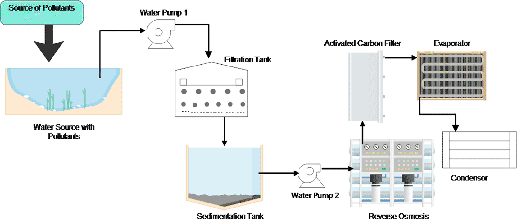
Figure 1 is a schematic of a multi-stage water treatment system for pollutant removal. Contaminated water from the source is first pumped into a filtration tank and then a sedimentation tank to remove suspended solids. The water then passes through an activated carbon filter for chemical adsorption, followed by reverse osmosis for fine purification. Finally, the evaporator and condenser stages complete the treatment, producing clean water suitable for use.
The system will be supported by solar power and its design will be done in the following ways:
i. Identify the overall load current and the operational time
ii. Add system losses
iii. Identify the solar irradiation in daily equipment sun hours
iv. Identify the PV array’s current requirements
v. Identify the optimum module arrangement for the solar array
vi. Sizing the battery for power storage
The loads of the pumps, evaporator and condenser are shown in Table 9. Whereas Table 10 indicates loads of two motor pumps, 1 evaporator and 1 condenser.
| Load (Device) | Power (W) | Voltage (V) | Current (A) = power/voltage | Daily usage (hrs) |
|---|---|---|---|---|
| Pump 1 | 250 | 230 | 1.09 | 2 |
| Pump 2 | 250 | 230 | 1.09 | 2 |
| Evaporator | 1000 | 230 | 4.35 | 4 |
| Condenser | 800 | 230 | 3.48 | 4 |
| Load | Capacity (watts) |
|---|---|
| Motor Pump (2) | 10 W |
| Evaporator | 20 W |
| Condenser | 20 W |
| Controller and Sensors | 10 W |
| Total = 60 W |
2.3.1 Energy Balance on a Solar Collector
This accounts for the solar energy received, absorbed, stored, and lost at the collector surface.
Where;
is the useful heat gain in Watts
is the incident solar energy absorbed in Watts
is the total heat losses (W), including convection, conduction, and radiation
2.3.2 Absorbed Solar Radiation
Absorbed Solar Radiation is the portion of solar energy that a solar panel surface absorbs after sunlight hits it. This kind of absorption is described in Equation 7.
Where;
A is the absorber area (m2)
G is the incident solar radiation (W/m2)
α\alphaα is the absorptivity of the surface (dimensionless)
2.3.3 Convective Heat Loss
Convective heat loss is the loss of thermal energy from a surface to the surrounding air, which carries particles that carry heat away from the solar panel surface. Equation 8 describes the heat transfer and panel surface temperature.
Where;
hc is a convective heat transfer coefficient in W/m2·K
Ts is a surface temperature measured in Kelvin (K)
Ta is the ambient temperature measured in Kelvin (K)
2.3.4 Radiative Heat Loss
Radiative Heat Loss is the thermal energy emitted by a surface in the form of infrared radiation, due to its temperature, toward a cooler surrounding (usually the sky or air) and depends on the emissivity of the surface, and is stated in Equation 9.
ϵ is the Emissivity of the surface, σ is the Stefan-Boltzmann constant W/m2.K4
The total heat loss is given in Equation 10
This calls for the energy balance in a Water Volume (Lumped System)
Where;
m is mass of water (kg)
cp is the specific heat capacity of water (J/kg·K)
is the Rate of temperature change (K/s)
2.3.5 Solar Collector Efficiency
Where;
η = Efficiency of the solar collector
2.3.6 The overall load current and the operational time
The normal operating voltage will be 12-24 V. Table 9 shows the loads in the water purification system and their daily working rates.
The total current, =
The Total Energy Demand per Day (ED) will be given in Equation 13.
Where;
is the power rating of the ith load (in watts)
is the Time, the ith load is operated per day
which is described in Equation 14.
Where;
is the total load power in watts
DoD is the Depth of Discharge, which is usually a capacity of 80%
2.3.7 How to Calculate Total PV System Losses
Figure 2,18–31 describes electrical components used in water treatment. The components helps in identifying the system power losses through determining load for each.
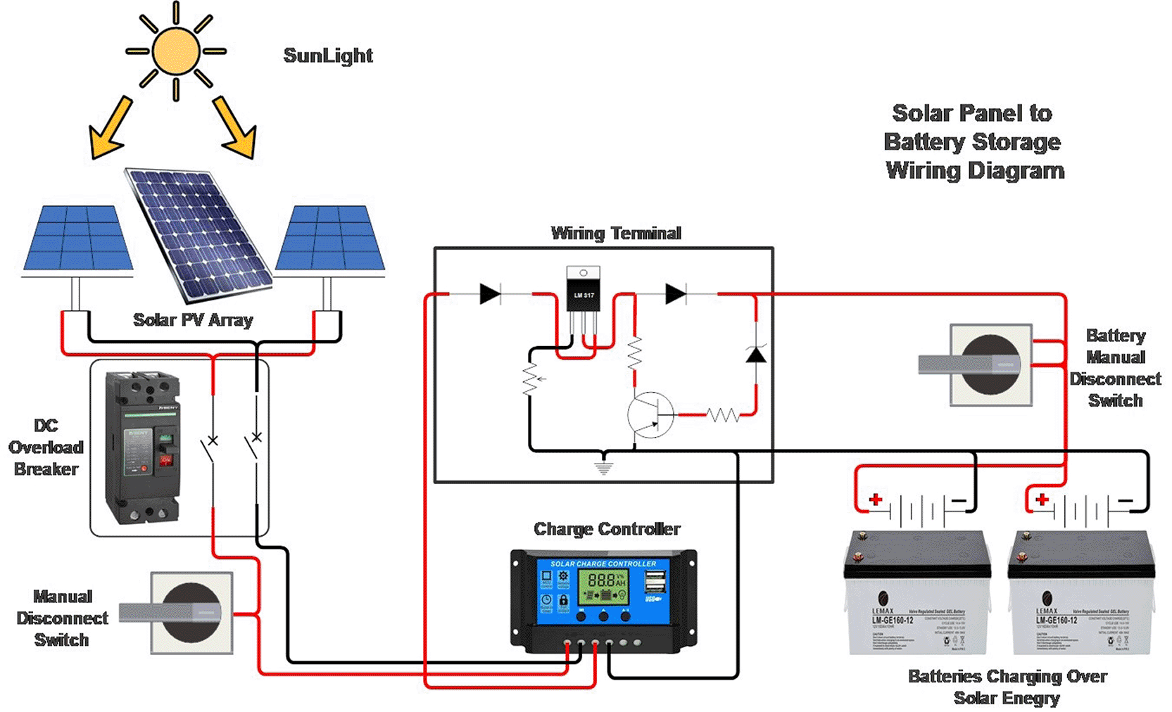
A schematic of the solar PV array charging system. The diagram illustrates the flow of solar energy from sunlight to battery storage. Sunlight is captured by the solar photovoltaic (PV) array, generating DC electricity. The generated power passes through a DC overload breaker and a manual disconnect switch for protection and safety. The wiring terminal and charge controller regulate voltage and current, ensuring proper battery charging. Energy is then stored in the connected battery bank, which can be manually disconnected as needed. This system ensures controlled and safe charging of batteries using solar energy.
2.3.7.1 Losses Inverter
The inverter will convert DC to AC. It provides a difference between the DC power input from the PV modules and the AC power output as shown in Equation 15.18
Where is the efficiency of an inverter which is determined by the manufacturer. According to PV Evolution Labs (PVEL) in 2019, the inverter power losses ranges from 2–5% and efficiency ranges 95 to 98%.
2.3.7.2 Soiling Losses
Accumulation of dust and dirt on the solar panels may cause losses, which are called soiling losses. Soil losses are identified using Equation 3.9
The formula for soiling losses (SL) will be given by
Where is the production energy when the PV has dirt (Joules)
is the production energy when the PV is clean from dirt in J or Watts
2.3.7.3 Losses caused by Temperature (T L)
This is the environmental temperature that is categorizes the ambient temperature, the level of irradiance, and the speed of wind. The effectiveness of solar cells decreases as the temperature rises. Equation 3.10 describes the factors that lead to temperature losses of the PV system.
Where;
is the module quality degradation factor
is the maximum energy/power at standard test conditions (Watts)
is the temperature coefficient
is the module temperature (0 C)
2.3.7.4 DC and AC cabling losses
The DC losses obtained in a PV system cannot be directly determined. For this solar water treatment system, the maximum current, IM, and maximum voltage are determined first to determine the cabling losses.19
Where where k is the Boltzmann constant 1.3806503 × 10⁻²³ J/°C, q = 1.60217646 × 10⁻²³ C is the charge of an electron. and G are temperatures (°C). =1000 W/m2 = irradiance of the standard testing condition. The other parameters will be used from the manufacturer’s manual.
The voltage difference in this DC will be obtained from Equation 19.
Where
is the measured voltage in volts. Measured at the inverter’s input.
The cabling losses (CDCL) are given in Equation 21.
Where the DC is current measured at the input point of the inverter.
is the PV module quality degradation factor.
2.3.7.5 Mismatch and wiring losses
This occurs when uneven panel performance and inter-cell/inter-module ohmic losses are obtained in the PV system. Equation 22 describes mismatch losses.
Where;
is the Power of the array with mismatch
is the Power of a perfectly matched array
Pa and Pi will be simulated using PVsyst
2.3.7.6 Wiring loss
Wire losses are caused by current with the wire, resistivity, and area of the wire as defined in Equation 23.
Where;
is the Resistivity of the wire material (Ω·m)
is the area of the cable wire (m2)
is the length of cable wire (m)
2.3.7.7 Degradation (annual)
As time goes on, the PV panel fades. The manufacturer indicates the degradation in a manual database. This will be used to identify the quality over time of the PV module.
2.3.7.8 Performance Ratio (PR)
This will help to determine the system’s availability. This will give the amount of sunlight required by the solar panel and convert to AC
According to,21
Where t is the time interval in hours
T is the total number of intervals
is the measured or actual AC output power of the PV system
is the rated power output of the PV module or system under Standard Test Conditions (STC)
is the Irradiance on the plane of the array at time t
is the Standard irradiance under STC, usually taken as 1000 W/m2
2.3.7.9 Shading Losses
Shading losses in a photovoltaic system refer to the reduction in energy output caused by the shadows of trees, buildings, poles, or masts, and the losses are described in Equation 25.
is the energy output of a PV system with shade (W/m2).
is the energy output of a PV system without shade (W/m2).
Extraterrestrial Solar Irradiance on a Horizontal Surface (
The amount of solar energy received per unit area on a horizontal surface at the top of the Earth’s atmosphere during a given time is described in Equation 26
Where:
Gs is the Solar constant (W/m2)
n is Day of the year (1–365)
Φ is Latitude (radians or degrees)
δ is the Solar declination (radians or degrees)
ω is the Sunset hour angle (radians or degrees)
The declination angle can be given as
2.3.7.10 Solar Irradiation on an inclined plane (Ht)
This is the amount of solar energy that strikes a tilted surface of a solar panel for a water treatment system over time and is determined in Equation 29.
Where H is the measured global radiation on the surface that is horizontal
is the Tilt angle
is the ground reflectance (typically 0.2)
Hb is the estimated beam
Rb is the ratio of the beam radiation on a tilted surface to a horizontal surface
Hd diffuse beam
2.3.7.11 Total Solar Irradiance on Collector Surface ( )
Where
is the total irradiance on the tilted surface [W/m2]
is the direct irradiance on horizontal [W/m2]
is the diffuse irradiance on horizontal [W/m2]
: Reflected irradiance, where ρg is ground reflectivity (0.2)
Β is the Tilt angle of the collector
R is the Ratio of the beam irradiance on tilted to horizontal
The current requirement will be determined by using the formula.
The system will be a 24 V voltage system
2.3.7.12 Solar Panel & Battery Sizing
Time required to treatment water per day
Daily energy = Total Load × Time required to treat water per day
The PV system is for 12 V
Proposed battery sizing = 25 Ah × 1.5 (safety factor) = 40 Ah
| Reynolds number | Flow regime | Notes |
|---|---|---|
| Re < 1 | Laminar | Darcy’s law is valid |
| 1 < Re < 10 | Transitional | Slight deviations from Darcy |
| Re > 10 | Turbulent | Inertial effects significant |
To determine the required capacity of the source, the daily water demand is estimated first.
Where N is the population of people to receive water
D is in m3/day
Q is per capita water consumption (Liters/person/day)
The flow rate,
Where T is the number of operating hours
Where
is the average daily demand?
is the peak demand factor, usually 1.8
Where the storage volume is used (m3)
is the surface area of the water body (m2)
is the effective depth of water (m)
Where A is the cross-sectional area of a pipe
Q is the flow rate
V is the velocity determined by the pump of the manufacturer
3.2.1 Pump Design
Where Q is the pump flow rate (m3/s)
D is the pump daily demand (m3/day)
T is the operating hours in a day
Where;
is the Suction head (vertical lift from source to pump)
is the delivery head (vertical height to the highest point in the system)
is the friction loss in the pipe
Or where Q is the flow (m3/s)
H is the Head (m)
= Water horsepower (Watts)
1 Horse power = 746 Watts
3.2.2 Hydraulic Power
The hydraulic power of a pump can either be static or dynamic, and it depends on the mass flow rate, the density of water, and the differential height.
Static hydraulic power from one height to another is given by,
Where s is the hydraulic power (W)
H is the maximum lift in meters. This is the head at the outlet
Q is mass flow rate (m3/s),
g is acceleration due to gravity, which is equivalent to 9.81 m/s2
Time, t, is in seconds
PS = Q , and Q = AV. Where A is area and V is velocity
Where A is the area of the cross-section and U is the initial velocity of water
The dynamic hydraulic power of a pump as water flows from one to another is given by,
, but so, , , maximum lift h.
Therefore static power of a water pump is equivalent to the dynamic power of a water pump.
3.2.3 Efficiency of a Pump ( )
Comparing electrical power with hydraulic power Water Pump, the efficiency of a pump must be greater than the efficiency of the system. Figure 3 illustrates a schematic of a pump, having a suction and an outlet pipe.32
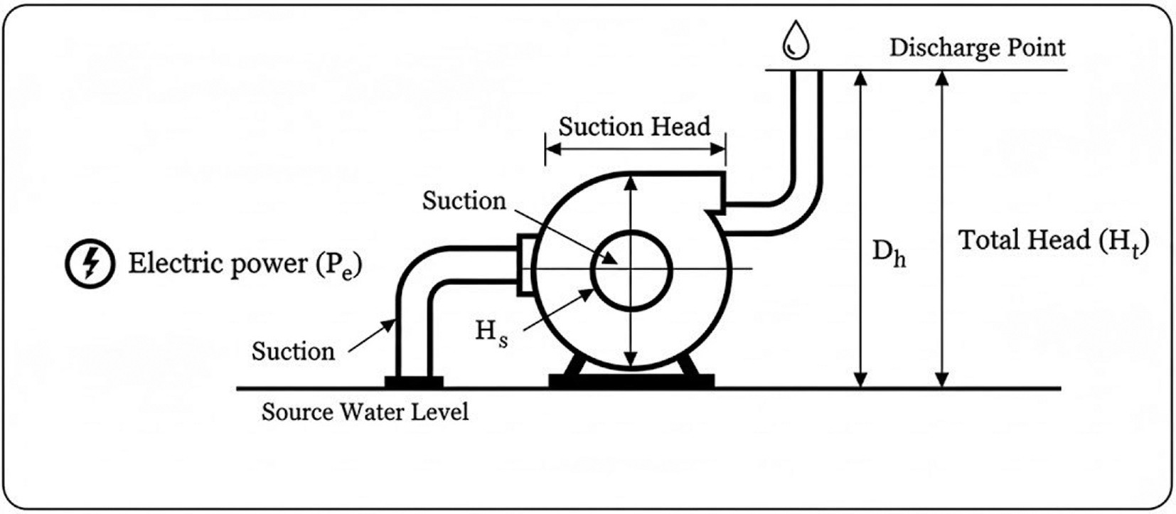
The architecture of Hydraulic Pump involving the direction of flow of liquid.
Electric power input of the motor will be equivalent to the electric power input Pe, of the pump. Considering the Figure 4 indicating a suction head of a pump, Sh, discharge head, Hs and total head Ht.32
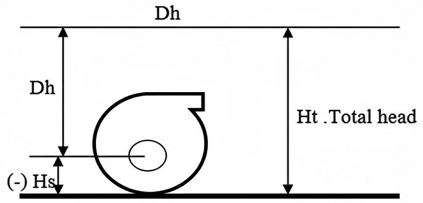
The architecture, show the total head pump.
Total head, Ht = Dh + Hs
From Equation 43
Considering the hydraulic power at a height of … … Therefore, power loss is
Efficiency of the system,
. Therefore,
The type of flow will be determined by
Where
ρ is fluid density (kg/m3)
u is the average fluid velocity (m/s)
D is the pipe diameter (m)
μ is the dynamic viscosity (Pa·s)
3.2.4 Modelling water flow using Navier-Stokes Equations
∇ is the Divergence operator
ρ is the fluid density (kg/m3)
u is the velocity vector of the fluid (m/s)
t is time (s)
For incompressible fluids
. This means density is constant,
Since the pipe is a 3D component, water will flow in 3D, and for 3D flow
Where u, v, w: velocity components in x, y, z directions
Conservation of momentum will be given as
Where;
f is the body forces
is the dynamic viscosity
ρ is the fluid density
p is the pressure
According to Roiti-Gromeka-Szymański ´nski Solution, the pressure gradient of laminar flow of water is given by the 51
Where r is the pipe radius, G is the pressure gradient.
The governing on how heat is transferred to water to kill micro-bacterial micro-organisms
The increase in temperature can kill more bacteria and micro-organisms. The heat energy required to kill bacteria is described in Equation 52.
Where;
is the amount of amount heat added. It is measured in Joules
m is the mass of water in kg
cp is the specific heat of water, which is equivalent to 4186 J/kg·°C)
ΔT is the temperature change in °C
When a phase change occurs, water boils, and the heat energy is converted as in Equation 53.
Where,
is the latent heat of vaporization
4.1.1 Inactivation models of microbial organisms
First-order of inactivation is described in Equation 54.
Where;
is the initial number of organisms
N is the number after time, t
K is the inactivation rate constant in 1/s
It is time in (s)
4.1.2 Time required to reduce microbial organisms (D value)
The higher the energy to inactivate bacteria, the less the time of inactivation.
Where;
D is the time required at a specific temperature to eliminate microbes by 90%
The temperature will change to the D-value
Where Z is the temperature increase needed to reduce the D-value by a log cycle
Where Qinput is the total heat supplied
q is the heat transfer rate in Watts
h is convective heat transfer coefficient in W/m2·K
A, area in m2
Ts, Tw are surface and water temperatures, respectively, in K
4.2.2 Fourier’s Law (Conduction)
Fourier’s law of heat conduction describes how heat flows through a solid material due to a temperature change, and it’s described in Equation 59.
Where K is thermal conductivity in W/m·K
is the temperature gradient
4.2.3 Transient Heat Transfer
Water is heated to an extent of it being unstable. The temperature change is explained in Equation 60.
Where
T0 is the initial temperature in Kelvin
is the Surrounding temperature
Ρ is the density of water
V is volume in cubic meters
T is time in seconds
The main purpose of a biosensor is to detect amounts of bacteria before and after treatment. The sensor will be used to detect the amount of oxygen in water that supports the growth of microorganisms. The BOD biosensor will determine the amount of oxygen in water, and will be oxidized by a microbial cell. The Clark-type oxygen electrode will be used as a transducer. The BOD will consist of a semipermeable membrane. Equation 63 describes the steady-state substrate balance in the biosensor used for measuring BOD
Where Du is the diffusion coefficient, which determines how easily bacteria and other microorganisms move through a semipermeable membrane in a BOD biosensor.
d is the thickness of the cell membrane
Sl and L are the concentrations of bacteria and other microorganisms in the external solution and the layer near the Clark-type electrode, respectively.
Vs is the rate of transport through the cell membrane at saturating concentrations of bacteria and other microorganisms
Ko is the saturation constant.
The relative concentration of the bacteria in the layer near the Clark-type oxygen electrode is given Equation 64
Where is the dimensionless module.
For extreme concentration of the substrate, the solution of at
at
The concentration of oxygen is stationary is obtained by the concentration of bacteria, which is equal to the flow of O2.
Where,
is the diffusion coefficient of oxygen and, W is the stoichiometric constant of bacteria
How to obtain the constant filtration rate
A filtration medium with the same cross-sectional area per a unit area, number of pores. Np with an average length lp and R radius respectively. As water flows into the filter, there is a possibilities of pore blockage and the particles accumulate on the membrane causing a cake.
Using Hagen-Poiseuille formula
The volume of filtered clean water is given as
The first filtration rate per unit area
The level of filtration (per unit area of filter medium) is
Where
Where
μ is the Dynamic viscosity of the fluid
is the length of the pores
If the mean radius of the pore decreases to R, then
The ratio of the new filtration becomes
Example of FTIR analysis of Polysulfone (PS) Ultrafilter static adsorption test.
During the filtration process of water, a reservoir with different-sized gravels is used. The Darcy law of flow of filtration is applied, while considering the volumetric flow rate, Q
Where
Q is the Darcy velocity
k is the intrinsic permeability of the medium (m2)
is the coefficient of viscosity
is the pressure difference in the direction of flow
To determine the type of flow, whether laminar, turbulent, or transitional. Reynolds’s number is computed as follows
In porous media, the flow is determined by the Table 11 below.
Microbial Load: Baseline analysis of 384 samples from Ishaka Municipality revealed critical levels of contamination. Escherichia coli was present in 72–85% of spring and wetland samples, with a mean concentration of 48–210 CFU/100 mL, significantly exceeding the WHO limit of 0 CFU/100 mL.
7.1.1 Chemical & Physical Profile: Turbidity levels ranged from 9 to 146 NTU (WHO limit <5 NTU), while Total Suspended Solids (TSS) were recorded between 18 and 92 mg/L. Chemical analysis detected heavy metals, including Lead (0.03–0.11 mg/L) and Arsenic (0.011–0.024 mg/L), alongside emerging contaminants like pharmaceutical residues (ibuprofen at 18–44 ng/L) and DDT pesticides (2–9 ng/L).
7.2.1 Solar Thermal Inactivation: Heating water to ≥70–100 °C achieved a Log Reduction Value (LRV) of 4–6 for E. coli. Complete bacterial inactivation was consistently reached within 8–12 minutes of sustained boiling.
7.2.2 Combined System Efficiency: The integrated system (Sedimentation + Filtration + RO + Thermal) achieved a cumulative removal efficiency of >95% across all contaminant classes.
Comparative Water Quality
Turbidity: Reduced from baseline 45–140 NTU to <2 NTU.
Heavy Metals: Lead and Arsenic concentrations were lowered to <0.005 mg/L and < 0.003 mg/L, respectively, well below regulatory thresholds.
7.3.1 Biosensor Validation: The integrated BOD biosensor exhibited a linear response range of 0–30 mg/L. Validation against standard laboratory BOD tests showed a high correlation coefficient (R2 = 0.89–0.94).
7.3.2 Response Dynamics: The sensor provided rapid real-time feedback with a response time of 45–90 seconds. Post-treatment monitoring showed a reduction in BOD from 4.8–11.3 mg/L to 0.9–1.8 mg/L, providing immediate verification of water safety.
7.4.1 PV Efficiency: The photovoltaic array produced 1.2–1.6 kWh/day, consistently meeting 100% of the system’s operational energy demand (1.0–1.3 kWh) even during low-irradiance periods.
7.4.2 Loss & Performance Analysis: Detailed loss modeling accounted for soiling (4–6%), temperature (3–5%), and inverter inefficiencies (2–3%), resulting in a final Performance Ratio (PR) of 0.84 to 0.88.
7.4.3 Hydraulic Stability: Navier–Stokes modeling yielded Reynolds numbers between 2,300 and 4,800, confirming transitional-to-turbulent flow that maintains stable volumetric flow rates across treatment cycles.
The results of this study demonstrate that the proposed solar-powered hybrid water treatment system is capable of effectively removing physical, chemical, and microbiological contaminants characteristic of rural surface water sources. The baseline analysis of 384 samples revealed high levels of turbidity, E. coli, heavy metals, pesticides, pharmaceuticals, and elevated TDS confirming widespread contamination consistent with reports from similar low-resource settings. These conditions justified the need for a modular, multi-stage treatment configuration capable of addressing diverse pollutants simultaneously.
The energy analysis further validated the feasibility of the system. The photovoltaic array, sized and modelled using real loss factors (shading, temperature, mismatch, soiling, inverter losses), produced sufficient energy to power the pumps, condenser, biosensor electronics, and heating components. The performance ratio (0.84–0.88) indicates strong operational efficiency for off-grid environments. This result is particularly important, as energy availability is one of the major barriers to water treatment in rural areas. A fully solar-driven system reduces operational costs and increases long-term sustainability.
The hydraulic modelling using Navier–Stokes and Darcy’s law provided insight into flow stability, filtration behavior, and pressure losses. The observed Reynolds numbers (2,300–4,800) confirmed transitional-to-turbulent flow within the system, which explains the stable volumetric flow rates delivered during treatment cycles. The sedimentation velocities and filtration permeabilities obtained experimentally matched well with the theoretical predictions, supporting the validity of the design approach.
A key innovation in this work is the integration of a BOD biosensor for real-time microbial risk monitoring. The biosensor showed a strong correlation with laboratory BOD results (R2 = 0.89–0.94) and responded within 45–90 seconds, offering a rapid, on-site assessment of microbial activity. The ability to detect biological contamination before and after treatment gives the system an advantage over conventional rural treatment units, which typically lack real-time quality verification. This integration transforms the system from a simple treatment device into a “monitor-and-treat” platform that improves safety and user confidence.
These findings collectively highlight that a unified, off-grid hybrid system can effectively address the multi-contaminant challenges present in LMIC rural water sources. Compared to existing decentralized systems which often treat only specific contaminants or rely on laboratory testing this design integrates energy, hydraulics, treatment, and biosensing into a single functional architecture.
However, the study has limitations. The system performance was modelled and validated using controlled conditions, and field variability such as seasonal fluctuations, turbidity spikes, long-term PV degradation, and membrane fouling may influence performance. Long-term pilot testing is therefore recommended to assess durability, maintenance needs, and cost-effectiveness. Additionally, the RO unit requires periodic membrane replacement, which may pose financial challenges in low-income communities unless supported by government or NGO partnerships.
Despite these limitations, the overall performance demonstrates the potential of this hybrid, solar-powered biosensor-integrated system to significantly improve safe water access in rural settings. By providing real-time microbial monitoring and multi-stage purification powered entirely by renewable energy, the system offers a scalable and sustainable solution that addresses both treatment and safety verification gaps in decentralized water management.
Table 12 indicates the treated water regarding the physiochemical parameters.
This work presents the development and modelling of a solar-powered hybrid water treatment system integrated with real-time biosensor monitoring for rural water purification. The analysis of 384 water samples from Ishaka Municipality confirmed that rural surface sources carry significant microbial, chemical, and physical contamination, underscoring the need for decentralized, multi-stage treatment solutions.
The proposed system successfully combines sedimentation, activated carbon adsorption, reverse osmosis, and solar thermal disinfection into a single off-grid architecture. Hydraulic, thermal, and solar energy modelling using Navier–Stokes Equations, Darcy’s law, Stokes’ settling theory, and solar energy balances demonstrated that the system operates efficiently under realistic conditions. The photovoltaic array produced sufficient energy to power all treatment stages after accounting for losses, confirming the viability of renewable energy for continuous operation in low-resource settings.
Treatment performance results show that the hybrid system achieves more than 95% overall removal efficiency across major contaminants, producing water that meets WHO drinking water standards. The integration of a BOD biosensor provided rapid, reliable microbial monitoring before and after treatment, transforming the system into a combined “monitor-and-treat” platform, an advancement not commonly found in rural purification technologies.
Overall, the system demonstrates strong potential as a sustainable, scalable, and autonomous solution for improving drinking water safety in underserved communities. Future work will include long-term field deployment, cost-benefit analysis, membrane fouling assessment, and user-centered design improvements to support community adoption and operational continuity.
| Views | Downloads | |
|---|---|---|
| F1000Research | - | - |
|
PubMed Central
Data from PMC are received and updated monthly.
|
- | - |
Provide sufficient details of any financial or non-financial competing interests to enable users to assess whether your comments might lead a reasonable person to question your impartiality. Consider the following examples, but note that this is not an exhaustive list:
Sign up for content alerts and receive a weekly or monthly email with all newly published articles
Already registered? Sign in
The email address should be the one you originally registered with F1000.
You registered with F1000 via Google, so we cannot reset your password.
To sign in, please click here.
If you still need help with your Google account password, please click here.
You registered with F1000 via Facebook, so we cannot reset your password.
To sign in, please click here.
If you still need help with your Facebook account password, please click here.
If your email address is registered with us, we will email you instructions to reset your password.
If you think you should have received this email but it has not arrived, please check your spam filters and/or contact for further assistance.
Comments on this article Comments (0)