Instrumented gait assessment with a single wearable: an introductory tutorial

Wearable technology: the mechanics

The common sensor within modern wearables comprises a tri-axial (medio-lateral, anterior-posterior, longitudinal) accelerometer: due to low manufacturing cost, miniaturised size and low power consumption⁸. Data digitisation and associated memory within the wearable, one full battery charge of a modern wearable is sufficient to gather data every 0.01s (100 Hertz) for 7 days. The equivalent of over 180 million (60 data point/second × 3 axis) data points to analyse a participant. Accelerometers quantify acceleration (measured in meters per second squared, m∙s^-2), calculated from the varying voltage generated within the sensor during movement (e.g. gait), for detailed functionality refer to 13. The signal generated is a combination of acceleration due to (i) dynamic conditions where each axis is perturbed due to 3-dimensional motion and (ii) static conditions where gravity has a pronounced effect on one axis of the tri-axial accelerometer (depending on attachment orientation) making this sensor useful for measuring static posture (lying, sitting, standing).

Wearable technology: current options

There is a plethora of commercial wearables for gait studies, e.g.: GaitUp (foot), Opal (ankle), StepWatch^™ (shank) and DynaPort (lower back). Each of the aforementioned may not offer the high sampling rates to gather ~180 million data points but all positives/negatives depending on the research question and provision of pre-programed outcomes. Nevertheless, all may be constraint by proprietary software and hence inbuilt data analytics. However, a recent shift by manufacturers has seen the (intellectual property) shackles loosened/removed to allow access to the ‘raw’ wearable data for bespoke analysis, facilitating attachment to any anatomical location (e.g. Shimmer^™)^14,15. This has been driven by the rapidly developing ‘open-source movement’, a concept of allowing access to all technical schematics, software scripts and algorithm descriptions. As such the potential for researchers (engineering/clinical) to analyse and interpret wearable signals has risen. One open-source wearable is the movement monitor AX3 (from Axivity; dimensions: 23.0 × 32.5 × 7.6 mm; weight: 9 grams), which allows access to raw data and is not constrained by one anatomical location. While that device is low-cost, no proprietary software exists to aid analytics from the signals that are generated.

The following section details the instrumentation of gait in any environment. While numerous devices have been highlighted, we present a methodology for a high resolution device (100Hz) worn on the lower back.

Instrumenting gait

Due to the miniaturised form factor of most wearables, they can be worn discreetly on almost any body location. As different accelerations are experienced at different anatomical locations, correct placement is of paramount importance when attaching the wearable¹¹. This is because algorithms used to investigate the signal and compute spatio-temporal outcomes are dependent on signal characteristics such as repeatable signal shapes/features. Typically, gait research has aligned to use of wearables located as close as possible to the centre of mass (CoM), i.e. the lower back (typically, 5^th lumbar vertebrae, L5). This best tracks whole body movement and for the purposes of instrumented testing a number of physical capability assessments and associated algorithms¹⁶. In another, it facilitates the use of a single wearable which reduces burden on the researcher and participant. This is of paramount importance during intervention or epidemiological studies where large patient numbers are recruited and tested^12,17,18. The following details a methodology for instrumented gait analysis that has been successfully implemented in several healthy and pathological studies^{8,10,12,18–20}.

Device attachment. Commercial devices are usually equipped with a strap/belt/clip for attachment. For the purposes of instrumented gait it is preferable that the wearable is attached as firmly to the participant as possible, eliminating spurious movement due to slippage. This usually requires direct attachment to the skin with a combination of dermatological adhesive(s) (e.g. Hypafix, BSN Medical Limited, Hull, UK) and double-sided tape. However, during prolonged testing, the participant’s skin (if frail/dry) can become compromised as a result of slight wearable movement due to lack of protection from thin double-sided tape. A solution is to adopt an adhesive hydrogel (e.g. PALstickies, PALTechnologies, Glasgow, UK) which provides additional padding due to its thicker design. Some motion artefact (slippage) and misalignment due to correct orientation and placement may be eliminated at the pre-processing stage from previously recommended procedures^21,22. Generally, under controlled gait assessment motion artefact is minimised due to a stringent and structured protocol. (Note: alternate locations (e.g. chest, waist) may be possible, depending on the robustness (suitability) of the algorithm used to accurately detect gait events for different locations other than from its intended use²⁰).

Protocol & gait characteristics. Validated instrumentation has shown that the use of a single wearable on L5 can capture 14 clinically relevant gait characteristics^10,16. Derived from a conceptual model (Figure 1a) they have been shown to be sensitive to age and pathology². Previous research suggests that the participant should perform a 2 minute continuous walk over a straight, or alternatively, looped path (Figure 1b) to record a sufficient number of gait cycles during steady state walking which improves the reliability of gait variability and asymmetry^1,3. If steady state walking is required then the first 2.5 m of walking should be excluded²³. If a testing environment doesn’t permit the use of a continuous walk, repeated intermittent walks and pooling of data is recommended. However, gait initiation/termination and their associated acceleration and deceleration periods may negatively influence results. This can be minimised by excluding the first and last steps (values) of the walks before pooling.

Figure 1.

(a) A conceptual model of gait showing 5 domains and 16 characteristics, M, A and V refer to mean, asymmetry and variability, respectively. 14/16 characteristics can be replicated with a single wearable worn on L5, step width (mean and variability) cannot. (b) A suitable path to test gait. The (suggested) 25m loop shown has sufficient linear paths to sustain steady state walking, while the curvilinear paths should be shallow enough to avoid abrupt directional changes.

Data import & segmentation. Matlab^® is a scripting programming language for general scientific computing that utilizes matrix oriented high-level programming for a large number of numerical tasks on many common platforms. Data processing can be achieved using existing and/or prototypic algorithms via script or command structure interfaces^24,25. Its support network (‘Matlab Central’), comprehensive toolboxes and ability to be translated to open-source languages (e.g. Python^TM, Octave) make it suitable for the processing of (gait) data into other programming software types^26–29. Therefore, for the purposes of this tutorial Matlab^® pseudo-code is provided.

Data must be downloaded from the wearable via associated software and saved securely. Data recorded by the wearable and saved by the proprietary software (including open-source) will typically be made available as a comma separated value (.csv) file due to its exchangeability. Importing the data to Matlab^® (Appendix 1, 1) can be achieved through the use of the xlsread function which offers the freedom to import data from a single or multiple column array(s) within a specified spreadsheet (Appendix 1, 2).

Once imported, data will automatically be saved to Matlab^® workspace as a variable. Typically some generic movement data will be recorded by the wearable during a testing session before/after the gait task and will need to be removed. If saved via a spreadsheet, erroneous data can be highlighted and deleted, trimming the data. If intermittent walks were performed, data can be segmented manually in the spreadsheet format prior to importing. (Note: Those familiar with Matlab^®, the ginput function can be used to segment data; enables user to define the exact start/end of the walk due to cursor point and click on a plot and save the x-axis values (samples/frames), Appendix 1, 3).

Data preparation: pre-processing. Data captured by wearables are subject to ‘noise’: random fluctuations in the signal due to connecting hardware and/or external interference. Removing noise can be achieved by filtering. There are many techniques one can apply to a signal (e.g. Butterworth, Chebyshev), each with their own advantages/disadvantages. Essentially, filters are deemed useful depending on how well they can remove the unwanted signal due to various associated parameters. Care must be taken when choosing those values as it may impact algorithm analysis, feature extraction. Nevertheless, the literature details the most common method as the 4^th order Butterworth filter with a cut off-frequency between 15–20 Hertz (Hz), Appendix 1(4). (For a comprehensive assessment of pre-processing of wearable gait signals refer to 30).

Correcting for offset & misalignment. When the wearable is attached to the participant, it is generally understood that the orientation or alignment of the device is offset due to attachment error and participant body shape. Additionally, gravity exerts a force, most notable on one axis. Attachment error and gravity can be easily overcome by asking the participant to remain still upon initial attachment and recording a few seconds of (quasi) static activity in a standing posture. The average/mean of the values captured by each axis in this posture is later subtracted from corresponding axes to eliminate offsets and misalignment.

However, this method is best suited to correct acceleration data in static postures only and not recommended for post-processing of gait data²². The correct approach is to transform the tri-axial data into a horizontal-vertical orthogonal coordinate system, i.e. using trigonometry relating to the Cartesian coordinate system^22,30. The methodology relies on calculating and correcting for the best estimates of the (offset/misalignment) angles (θ) between the true horizontal-vertical and that of the raw anterior-posterior (a_a) and medio-lateral (a_m) accelerations. While the accelerometer within the wearable cannot provide the rotational angle (gyroscopes), it is deduced²² that the average value of a_a and a_m will approach the sin of the angles within the same directions, Equation 1–Equation 4 (translated code Appendix 1, 5). By applying the inverse sin (arcsin) methodology, one can derive the necessary values needed to correct offset/misalignment in four straightforward, recommended³⁰ steps:

The above is achieved through mean, sin, cos and arcsin functions along with basic matrix multiplication (Appendix 1, 5).

Algorithms. Methodologies have been developed to quantify temporal and spatial characteristics for a wearable on L5, comparisons can be found here³¹. All aim to identify two features of gait: initial contact (IC, i.e. heel strike) and final contact (FC, i.e. toe off), Figure 2a. A robust temporal method³¹ uses wavelets³². This methodology is a powerful signal processing tool that has been used successfully in gait and postural transition analysis^32–34, yet its use remains limited due to complexity. The basic premise is that it offers an extension on the Fourier transform by two procedures: continuous (CWT) and discrete (DWT) wavelet transforms. Detailed descriptions is beyond the scope of this manuscript, but can be easily described; (i) CWT: a correlation between waveforms (raw signal and probing function, i.e. wavelet) at different scales (~ frequencies) and positions (in time), where the resulting coefficients roughly correspond to the best match; and (ii) DWT: a combination of high/low pass filters to divide up a (raw) signal into various components. (see 35 in depth descriptions refer to). Nevertheless, implementing a CWT algorithm³² for IC/FC event detection can be relatively straightforward if utilising the Wavelet Toolbox within Matlab^®, Appendix 1(6):

Figure 2.

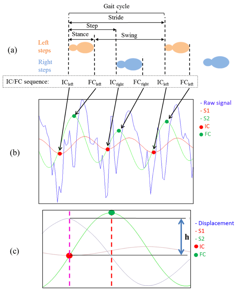
Gait signal from a young healthy adult (a) The gait cycle with depictions of stride, step, stance and swing characteristics from the IC/FC events (b) The raw signal (a_v), integrated and differentiated CWT signals with corresponding IC/FC events. The IC/FC sequence must be amalgamated into one numerical array from the alternating peaks/troughs to estimate the correct timing sequence for stride, step, stance and swing times. (c) Step length can be derived using Equation 5, where h is derived from change of wearable height due to double integration of vertical acceleration (implementing cumtrapz function twice).

Temporal characteristics. To fully replicate the characteristics of gait: step, stance, stride and swing times must be derived. This is achieved through the sequence of IC/FC events in relation to the double support phase of the gait cycle (see Figure 2). From the sequence (i) of IC/FC events, both left and right (opposite) events are identified, and subsequently step, stride, stance and swing times are estimated (Equation 5–Equation 8). For full details of calculating these parameters see 10,36.

Spatial characteristics. A spatial algorithm based on the inverted pendulum model tracks the CoM³⁷. However, the model is reliant on a known variable, wearable-height. This manual component is a weakness: requiring a known input and can have weak accuracy for step length or total distance walked^8,12. Yet it remains a useful metric to compute via the simple relationship shown in Equation 5, where l is wearable height and h is change in height of the wearable (i.e. CoM) as the participant walks, Appendix 1(7). Subsequently, by fusing the algorithms from Figure 2^8,10, it is possible to quantify an estimate for step velocity (Equation 6 and Appendix 1, 7). However, implementing the cumtrapz function to derive velocity and speed from acceleration introduces an error known as drift. This can be eliminated through the use of filtering, but generally remains problematic within wearable gait analysis.

Variability and asymmetry characteristics. It is useful to distinguish between left/right step characteristics for variability and asymmetry outcomes (Equation 11 a, b and 12, Appendix 1, 8) in asymmetrical diseases³⁸. Differentiating between left/right during a long continuous walk is easier (assume first as left or right and alternate values thereafter) compared to repeated intermittent walks when (for robustness) it would be recommended to note what foot was used for initiation⁸. Alternatively, a protocol could request the participant initiates walking with the same foot. Subsequent assignment of values to left/right can be made during data analysis by manually dividing the data. (For the readers interest, left/right steps may be identified by automated but more complex algorithms and can be found here: 32,37). Correct calculation of variability^1,10 and asymmetry is performed by:

or

                                                                    Variability= SD(Steps)                                                                                                                                      (7b)

                                                                    Asymmetry_{left & right} = |average_left – average_right|                                                                                              (8)