Using complex networks for refining survival prognosis in prostate cancer patient

Network reconstruction

Reconstructing a network representation of a given system entails two steps. First, one needs to define the elements of such a system. This is usually constrained by the type of available data; thus, in this case, the nodes of the network are going to correspond to the different available biomarkers.

Second, one should detect when two of such elements are connected by some kind of relationship. If a priori knowledge is available, e.g. information about how different metabolites or proteins are connected in a pathway, such information can directly be mapped into the network. Alternatively, if a time evolution (i.e. a time series) is available for each element, functional links can be established between them, by means of metrics like correlations or causalities. Note that this last option entails two important problems: a time evolution should be available, which is not straightforward in the case of biomedical analyses; and that functional links represent the “co-evolution” of factors, while in some cases, and specifically in the diagnosis of a disease, it is more interesting to detect “deviations” from the expected (healthy) behavior.

Recently, a new methodology for network reconstruction has been proposed, which solves the two aforementioned problems (Zanin & Boccaletti, 2011; Zanin et al., 2014). Starting with a set of scalar values, pairs of elements are analyzed by firstly detecting if a standard relation is present between them in a set of control subjects; afterwards, data corresponding to new subjects are compared with such relation, and a link is created between two nodes if they present an abnormal deviation. The resulting object is called a parenclitic network, named after the Greek term for “deviation”, originally used by the Greek philosopher Epicurus to designate the spontaneous and unpredictable swerving of free-falling atoms (Zanin et al., 2014).

In mathematical terms, suppose n healthy subjects are described by a vector of features, such that the i-th of them is represented by f_i = (f_i,1, f_i,2, … , f_i,nf). All the n_f features are mapped into nodes of the network, which is now described by an adjacency matrix A_nf×nf. As the final aim is to construct a network for each subject under study, suppose a new subject j, with its corresponding vector f_j, is introduced in the system. The reconstruction process should analyze each pair of features, denoted by k and l, to understand if they deviated from the expected (healthy) behavior. For the sake of simplicity, in this work we consider that the healthy relation can be obtained as a linear regression between both features:

                                                                                                       f._,l = α_k,l + β_k,lf._,k + ∈_k,l.

Here, f._,k represents the vector of values of feature k for all healthy subjects, and α_k,l and β_k,l the two parameters of the best linear fit. Additionally, ∈_k,l is a vector containing all fit errors; note that a linear relation may not describe well the relationship between k and l, and that this vector will be key to understand its statistical significance. Now, suppose a new subject h is available, for which their health condition is unknown, and for which one wants to create the corresponding network representation. A link between nodes k and l is then created, with a weight equal to its distance from the previously detected normal relation:

$$w_{k,l}=\frac{f_{h,l}–\left({\alpha }_{k_{,}l}+{\beta }_{k_{,}l}{f}_{h,k}\right)}{{\sigma }_{k,l}},$$

being σ_k,l the standard deviation of ∈_k,l. In other words, w_k,l represents the Z-score of the distance of the subject h with respect to the normal behavior of features k and l - large values of w_k,l, both positive and negative, indicate that the subject under analysis presents an abnormal behavior, which may be symptomatic of a disease. When the process is repeated for all pairs of features, the result is a parenclitic network for each patient.

Network interpretation

Intuitively, healthy subjects should be associated with random-like networks, as strong links may appear due to the intrinsic noise of biological processes, but should not form coherent structures; on the other hand, patients should present networks with non-trivial topologies. Also, the more a network is different from a random structure, the more severe the pathology is expected to be.

In order to transform the obtained networks into a representation suitable to be used in a data mining (classification) algorithm, first these have been binarized, i.e. links with a weight |w_k,l| ≤ 0.5 have been discarded. The threshold of 0.5 has manually been set, in order to obtain structures dense enough to support the subsequent analysis, but still being able to discard statistically insignificant connections. Afterwards, two topological (i.e. structural) properties have been considered:

Classification

In order to evaluate the performance of a complex network representation with respect to a baseline, a classification between the two groups of patients (i.e. surviving vs. not surviving patients) is performed, and the resulting scores compared. Such classification is based on a support vector machine (SVM) model with linear kernel (Noble, 2006; Wang, 2005).

SVMs are binary linear classifiers that model concepts by creating hyperplanes in a multidimensional space, which can be used for both classification and regression (Cortes & Vapnik, 1995). A good separation is achieved by the hyperplane that has the largest distance to the nearest training-data point of any class, as this minimises the error. The SVM model has been chosen for two reasons: its good performance and diffusion in biomedical classification problems; and its simplicity: only linear relationships are mined, allowing a better identification of the contribution of the complex network representation.

The validation of the results has been performed using a 10-fold cross-validation (Friedman et al., 2001). The original sample of subjects is randomly partitioned into 10 equal sized subsamples. A single subsample is retained as the validation data for testing the model, and the remaining 9 subsamples are used as training data. The cross-validation process is then repeated 10 times, with each of the 10 subsamples used exactly once as the validation data. The average value of the error obtained in the 10 executions is used for estimating the error.

Initial dataset

The dataset considered here is part of the Prostate Cancer DREAM Challenge, including information from the prostate cancer clinical trials ASCENT-2 (Novacea, provided by Memorial Sloan Kettering Cancer Center) (Scher et al., 2011), VENICE (Sanofi) (Tannock et al., 2013), MAINSAIL (Celgene) (Petrylak et al., 2015), and ENTHUSE-33 (AstraZeneca) (Fizazi et al., 2013). Only the data included in the CoreTable have been considered, representing the core patient level data. They cover information about demographics, co-existing disease conditions, prior treatment of the tumor and other co-existing conditions, important baseline lab results and vital signs, lesion measure and early response to therapy. More information on the dataset can be found at https://www.synpase.org/ProstateCancerChallenge.

One of the limitations of the network reconstruction process previously described is that it can only handle numerical features. Thus, only those features fulfilling this condition have been selected. Additionally, binary features have been transformed into numbers, i.e. 1 for “yes” and 0 for “no”. The final data set included 92 features for each patient.

Afterwards, 2000 patients have been randomly selected, of which half of them did not survive cancer - as coded by the DEATH flag in the dataset. The rationale of selecting only a subset of patients is two-fold: first, to reduce the computational cost, and thus allow a more detailed analysis of results; and second, to ensure that the data set used in the classification task is balanced, i.e. it includes the same number of subjects in both classes. All other patients have been discarded.

Standard scenario: raw features classification

Figure 1 presents the results obtained in the classification of patients using only raw features. As previously introduced, this classification will be the baseline against which the benefits of using complex networks will be evaluated. In order to reduce the computational cost of the analysis, and to reduce the risk of overfitting, a greedy feature selection algorithm has been executed. The three selected features were: LDH (Lactate Dehydrogenase level), TURP (prior transurethral resection of the prostate, binary value) and MHGEN (presence of general disorders, binary value). The probability distributions for the three features are presented in Figure 1 top and bottom left.

Figure 1. Classification with raw features.

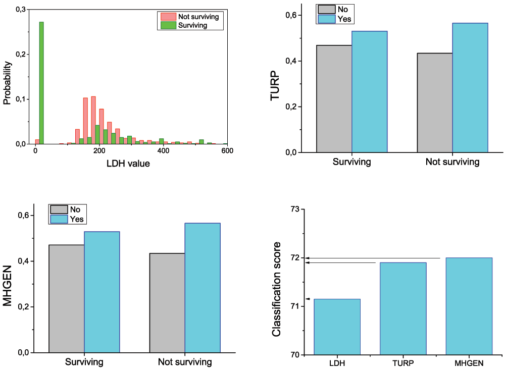
Probability distributions of the LDH feature for surviving and not surviving patients (top left). Appearance probability of the features TURP and MHGEN, for surviving and not surviving patients (top right and bottom left). Classification score when considering LDH, LDH + TURP, and all three features (bottom right).

By using these three selected features, the classification score reaches 72.1% (Figure 1, bottom right). Adding more features does not yield substantial improvements.

Enhanced scenario: complex network features

In the second case, I consider the same original raw features, plus the two features synthesized from the complex network representation, as previously described. A network has been created for each subject, by using the information of surviving patients as baseline- in other words, surviving patients have been considered as healthy, following the convention previously described. In order to avoid overfitting, a new baseline has been calculated in each one of the 10 cross-validation rounds, ensuring no patient was included both in the training and in the classification steps. Finally, a greedy feature selection algorithm has been executed on the complete feature set, following the same process described previosuly.

Figure 2 presents the results obtained, both in terms of the network features probability distributions (top), and the classification score (bottom). It can be appreciated as the classification score improves, from 72.1% up to 76.2%; this corresponds to a decrease of 15% in the classification error.

Figure 2. Classification with complex network features.

(Top) Probability distributions of the link density and Information Content features, for surviving and not surviving patients. See main text for definitions. (Bottom) Classification score when considering LDH, LDH + link density, and all three features.