Keywords
Measurement error, Internal validation study, Attenuation, Bias, Questionnaire data, Sensitivity analysis, Error correlation
Measurement error, Internal validation study, Attenuation, Bias, Questionnaire data, Sensitivity analysis, Error correlation
HIV: Human immunodeficiency virus; HBCT: Home-based HIV counseling and testing; HSRC: Human sciences research council; NCD: Non-communicable diseases; BMI: Body mass index; kg: kilogram; m2: metre squared; g: gram; MCMC: Markov Chain Monte Carlo; CI: Credible interval; JAGS: Just another gibbs sampler; BUGS: Bayesian inference using gibbs sampling; ACF: Autocorrelation function
Difficulty in obtaining correct measurements of an individual’s long-term exposure is a major challenge in an epidemiological study that investigates the association between a continuous exposure and a health outcome. For instance, several studies estimated the correlations between self-reported intake from a questionnaire and the true long-term intake values to be less than 0.82 for fruits and about 0.72 for vegetables1–5, an implication that some of the variation in the diet intake measurements is due to random errors. Due to random error, the association between the dietary intakes and health outcomes may be biased. The effect of measurement error can be quantified using either: (i) the attenuation factor, which quantifies the bias in the association or (ii) the correlation coefficient between the true and the observed exposure, which quantifies the loss of statistical power to detect a significant association (i.e. validity coefficient)6.
Validation studies are used to assess the accuracy of the dietary questionnaire6–12. A validation study constitutes a small number of individuals from whom dietary intakes are measured repeatedly using an unbiased instrument13. There are two types of validation studies: the external and internal validation studies. An internal validation study is conducted on a subset of individuals from the main study, whereas an external validation study is carried on a group of subjects who are not part of the main study, but who are similar in characteristics to individuals in the main study. Validation studies are often expensive to conduct and, in some cases not feasible. Several methods have been proposed to handle measurement error in the absence of internal validation data14–18.
Agogo et al.14 conducted a sensitivity analysis to investigate the effect of the magnitude of the correlation between errors in the covariates of interest and found that the magnitude of measurement error adjustment is sensitive to the assumed measurement error structure. Dellaportas and Stephens15 presented a Bayesian method for analysis of non-linear error-in-variable where prior knowledge of the unknown true covariate is incorporated. Huang et al.16 proposed a quantile regression-based non-linear mixed-effects joint models for longitudinal data that simultaneously accounts for a response with non-central location and for covariate with non-normality and measurement error under the Bayesian framework. Lin17 proposed a Bayesian semi-parametric accelerated failure time model to analyze censored survival data with covariate measurement error and evaluated their method using an intensive simulation study. Muff et al.18 introduced a Bayesian method to handle a mixture of classical and Berkson measurement errors in a single explanatory variable and illustrated their method to studying cardiovascular disease mortality.
The majority of these authors considered a case where one exposure is measured with error (hereafter, a univariate case). In a univariate method, the bias in the association between an outcome and the exposure is adjusted by dividing the unadjusted association estimate by the attenuation factor19. An attenuation factor is the ratio of the variance of the true exposure to the variance of the observed exposure. This method ignores correlations between the errors, which can lead to substantial bias. In this study, we suggest a general method for adjusting for measurement error where multiple exposures are measured with correlated errors in the absence of an internal validation study (hereafter, a multivariate method). We use real data to illustrate the method in handling a case where three exposures are measured with correlated errors (hereafter, the trivariate method) under a linear regression model and demonstrate the implementation of this method using R software20. Specifically, we use a subset of data from a home-based HIV counseling and testing study that was done in rural and peri-urban communities in KwaZulu-Natal Province, South Africa21. We compare the results obtained when using a method that ignores both the measurement error and correlation between the errors (hereafter, a naive method) with those obtained when using univariate and multiple exposures methods. Moreover, we conduct a sensitivity analysis to investigate how the coefficient estimates of parameters of interest are influenced by (1) a change in the level of uncertainty assumed for the limits of the validity coefficients and (2) varying the correlation between errors in the measured exposures.
The remaining sections of this paper are organized as follows. In section 2, we discuss materials and methods used in this study. We present the results of the study in section 3. Finally, we provide a discussion and conclusion in section 4.
In this work, we use a subset data from a home-based HIV counseling and testing (HBCT) study that was conducted in rural and peri-urban communities in KwaZulu-Natal Province, South Africa, between November 2011 and June 201221. The data were obtained from the Human Sciences Research Council (HSRC) of South Africa21. This study was conducted to provide a better understanding of the complexity, severity, and prevalence of non-communicable disease (NCDs) in a community known to have one of the highest rates of HIV incidence and prevalence in the world21.
Home-based HIV counseling and testing is a cross-sectional, single-site study in South Africa that aims to increase engagement in HIV care by integrating NCDs screening with community-based HIV testing22. A random sampling approach was used, where 587 participants over the age of 18 were selected from 50,000 people living in the Mpumuza suburb21. Anthropometric and biological measures were collected in the survey with the purpose of establishing the prevalence of a range of NCDs and associated risk factors. Eligible individuals participated in a face-to-face interview, physical, psychological and clinical examinations. Persons younger than 18 years living in Mpumuza and all household members not previously enrolled, and members unable to give written consent were excluded from the study. Mobile phones were used for data collection to increase efficiency in data capture and analysis21.
In our study, we used a subset data consisting of 76 individuals who self-reported the number of cigarettes smoked, fruit and vegetable consumption. We use the dataset to illustrate the multivariate method in modeling the amount of association between body mass index (BMI) and three exposures (smoking, fruit, and vegetable intakes). BMI was measured in kg/m2, while smoking was measured as the average number of cigarettes smoked per day. Initially, fruit and vegetable intakes were measured in terms of the number of servings consumed per day. It is often assumed that a standard portion of fruit/vegetable weighs about 80g5. Therefore, for this study, we converted the number of servings to grams per day (g/day) by multiplying the reported number of servings by 80g. The subset data has the following three properties that make it suitable for use in this work: (1) measurement error in the recorded number of cigarettes smoked due to possible misreporting, (2) measurement error in fruits and vegetable consumption due to recall bias, and conversion of the number of servings of fruits and vegetables into grams, and (3) the measurement error in the three exposures is often correlated, for instance, smokers are likely to over-report fruit and vegetable intakes due to their beneficial effects, and to under-report the number of cigarettes they smoke due to the associated harmful effects. Epidemiologically, BMI is used as a risk factor of a health outcome. However, in this study, we model BMI as an outcome as in other several studies, for instance,23–26. The subset data is only used to illustrate the method and not to draw inference.
Ethics approval was granted by both HSRC Research Ethics Committee (REC: 1/26/05/11) and the University of Washington Institutional Review Board (48733). Informed written consent was obtained from each participant in the study. Participants were provided with written information on the study (including the study’s background and objectives) and their rights regarding participation and withdrawal at any time.
An interest in epidemiological study could be to investigate the association between BMI and three exposures namely: fruit, vegetable and smoking using the multiple linear regression
where Y denotes the BMI, β0 is the intercept, βX1, βX2 and βX3 are the coefficient parameters for the true long-term fruit (X1), vegetable (X2) and cigarette (X3) intake respectively and ϵ is the random error term. In this study, we use vegetable intake and cigarette smoking as confounders and assume that the main interest is in estimating βX1. In practice, the true intakes are unobservable and, therefore, the intakes recorded in self-reported questionnaires are used. Let W1, W2 and W3 denote the measured versions of X1, X2 and X3, respectively. The use of Wp’s in place of Xp’s, (p = 1, 2, 3), in Equation (1) yields biased estimates , and of βX1, βX2 and βX3 respectively. Let
We assumed that the observed exposures are related to the true exposures with additive measurement error as
where ϵW = (ϵW1, ϵW2, ϵW3)⊤, ϵW ∼ N(0, ΣϵW); W = (W1, W2, W3)⊤; α0 = (α01, α02, α03)⊤, α1 = (α11, α12, α13)⊤; with the terms in α0 and α1 quantifying the constant bias and the proportional scaling bias respectively; ϵW is a random error term, ϵWi is assumed to be independent of the true exposure Xi and the systematic bias components, α0i and α1i.
A univariate method. In a univariate case, the bias in the association between an outcome and an exposure is adjusted by dividing the unadjusted association estimate by the attenuation factor19. Attenuation factor (λi) is defined as λi = var(Xi)/var(Wi), i.e., the ratio of the variance of the true exposure to the variance of the observed exposure, also referred to as reliability ratio. This method ignores correlations between the errors and also the correlation between the true exposures.
Multivariate method. We propose and describe a general approach for handling p-exposures (p≥2) measured with correlated errors. For simplicity and without loss of generality, we assume that Wi is measured without systematic bias (i.e., α0i = 0, α1i = 1 in Equation 2). For multiple exposures measured with correlated errors, the adjusted association estimates can be obtained by pre-multiplying the unadjusted association estimates by the inverse of the transpose of attenuation-contamination matrix as
where and denotes vectors of true and biased coefficients for the p-exposures respectively and Λp denotes a p × p attenuation-contamination matrix19,27. The off-diagonal elements in Λ are known as contamination factors while the diagonal elements are called attenuation factors14. Noteworthy, the attenuation factor quantifies the bias in the association between an outcome and an exposure. In contrast, the contamination factor quantifies the effect of measurement error in one exposure variable on the other exposure variable’s estimate. in Equation (3) can be obtained from the observed questionnaire data.
In the multiple exposures case, the estimate of attenuation-contamination matrix is defined as
where is the estimate of covariance matrix of the true exposures, is the inverse of the estimate of covariance matrix of the measured exposures, is the variance estimate of Xi (i = 1, 2, ..., p) ; (j = 1, 2, ..., p; i ≠ j) denotes the covariance estimate between the true exposures; is the variance estimate of Wi; (i ≠ j) is the covariance estimate between the observed exposures.
The elements of the variance-covariance matrix of the observed exposures, , are estimated from the observed data. The variances of the true exposures, ’s, can be estimated using validity coefficients for the questionnaire. According to Kipnis et al.6, the validity coefficient is given by:
where Wi is assumed to be the measured with error term only and ϵWi is assumed to be independent of Xi. From Equation (5), we estimate the variance of the true exposures as
by incorporating external validation information on ρWiXi. To obtain covariances between the true exposures, one of the following two approaches is used: (i) if external information about the correlation between true exposures (i.e. ) is available, we obtain covariances between true exposures as follows:
where are obtained as shown in Equation (6); (ii) if we can obtain prior information about the correlation between the errors in the observed exposures, we can solve for by decomposing the covariance of observed exposures into unknown covariance between true exposures and unknown covariance between errors as follows:
where Xi and ϵWj, Xj and ϵWi are assumed to be uncorrelated.
From Equation (2) and Equation (6), the estimate of the error variance is
See Appendix B of the extended data28 for the proof.
From Equation (8)–Equation (9), the covariances between the true exposures are given by
Using the observed data and external information, we can determine all the terms required to estimate the attenuation-contamination matrix, Λ, as shown in Equation (4) and adjust for the bias in the association between the exposures measured with error and the outcome using Equation (3).
We illustrate a method that accounts for uncertainty in the validity measures attributable to heterogeneity in the study populations and in parameter estimation. The proposed Bayesian method applies Markov Chain Monte Carlo (MCMC) estimation approach to combine observed self-reported data and external validation data in adjusting for measurement error in three exposures measured with correlated errors. MCMC is a class of algorithms that samples from the posterior distributions by traversing the parameter space29. The posterior distribution is obtained by updating the prior distribution with observed data. The steps for implementing the trivariate method are described below.
We first obtained external information on validity coefficients and generated validity coefficients for use by interpreting the lower and upper limits obtained from the literature as the 95% credible intervals (CIs) of the distribution of possible values respectively. Due to the skewed distribution of validity coefficients, Fisher’s transformation was used to generate the validity coefficients as explained in the next section.
Second, for the observed exposures, we estimated the posterior distribution of the covariance matrix (ΣW). The exposures were assumed to follow a multivariate normal distribution with mean and covariance, i.e., W ∼ N3(µW, ΣW). We assumed a weakly informative multivariate normal prior for µW as µW prior ∼ N3(0,106 I3), where I3 is a 3 × 3 identity matrix. In a multivariate normal distribution, ΣW must satisfy two conditions: (1) be positive definite (i.e. WTΣWW > 0, for all W) and (2) be a symmetric matrix. The semi-conjugate prior distribution for ΣW, which has these two properties, is the inverse-Wishart distribution29. To minimize the influence of the prior information on the estimate of ΣW, we considered weakly informative inverse-wishart prior as ΣW prior ∼ IW(I3, v), where v = 3 is the degrees of freedom.
Third, using the validity coefficients generated from the external data and the posterior distribution of covariance matrix for observed exposures, we estimated the variance of true intakes, (i = 1, 2, 3), using the relationship given in Equation (6) so that
The covariances between true intakes ( ; j = 1, 2, 3) were estimated as,
by incorporating external validation information on correlation between the errors (ρϵWi ϵWj). We generated the correlation between errors from a plausible range guided by correlation in the observed data and prior expert information on the most likely sign of the correlation between the exposures, as described in the next section.
Having obtained the covariance matrices of the true and observed exposures, we estimated the attenuation-contamination matrix (Λ3) from their joint distribution as
where is the estimate of covariance matrix of the three true exposures, is the inverse of the estimate of covariance matrix of the three measured-with-error exposures, is the variance estimate of Xi (i = 1, 2, 3); (i ≠ j) denotes the covariance estimate between the true exposures; is the variance estimate of Wi; (i ≠ j) is the covariance estimate between the observed exposures.
Lastly, we fitted a Bayesian multiple linear regression model (hereafter, naive method) to obtain the posterior distributions of the unadjusted coefficient estimates In the naive model, we assumed weakly informative normal independent priors by choosing a very small precision (large variance) for the unadjusted coefficient estimates as βWi prior ∼ N(0, 106). The adjusted coefficient estimates were then obtained from the joint posterior distribution of and as
We implemented the trivariate method in R version 3.6.3 using rjags (version 4-10), coda (version 0.19-3), MCMCpack (version 1.4-9), and mvtnorm (version1.1-1) packages. To facilitate Bayesian estimation of the covariance matrix of the observed exposures (ΣW), rjags package was used to provide an interface from R to the JAGS library30. JAGS is a gibbs sampler that uses MCMC to draw dependent samples from the posterior distribution of the parameters31. The Bayesian estimation of ΣW proceeded in the following steps: (1) defining a model for ΣW under Bayesian inference using gibbs sampling (BUGS) algorithm in a stand alone file, (2) reading the model file using the jags.model function, (3) updating the model using the update method for jags objects and (4) extracting the posterior samples of the model using the coda.samples function from the coda package.
MCMCregress function from the MCMCpack package was used to generate a posterior density sample from the naive linear regression model32. MCMC convergence diagnostics of all the model parameters was done using trace plots and autocorrelation (ACF) plots from the coda package33. See extended data: Appendix C28 for convergence diagnostics results. For each model, the burn-in iterations were set to 2,000 and 10,000 MCMC iterations were run after the burn-in iterations. Every first sample value was kept in the MCMC simulations by using a thinning interval of 1. When compiling a JAGS model, an initial sampling step may be needed during which the samplers learn their behaviour to maximize their performance34. Therefore, the number of iterations for adaptation in the the jags model was set to 500. The results were presented in terms of density plots, posterior mean and median. We compared the results obtained under naive, univariate, and trivariate methods. The R code used for analysis is presented in the extended data28.
External information on the validity coefficient and error correlations for fruit, vegetable, and cigarette information was obtained from the literature. According to Kaaks et al.1, the validity coefficient of self-reported fruit intake ranges from 0.33 to 0.79, while that of vegetable intake ranged from 0.30 to 0.60. A meta-analysis study on the validity of questionnaires assessing fruit and vegetable consumption by Collese et al.2 reported validity coefficients of 0.26 for vegetables and 0.49 for fruits. Other similar validation studies reported validity coefficients in the aforementioned ranges for fruits and vegetables3,4,35. Therefore, based on these information we considered a range of 0.3 to 0.8 for fruits and a range of 0.25 and 0.7 for vegetables.
In the Scottish Heart Health Study of 2,849 men and 2,900 women36, the correlation between the self-reported number of cigarettes and biochemical measures was reported between 0.67 and 0.72. In a study on the validation of self-reported smoking by analysis of hair for nicotine and cotinine37, the validity coefficient between the number of cigarettes smoked per day and nicotine/cotinine levels in hair and plasma was found to be between 0.48 and 0.63, while the correlation between the average number of cigarettes smoked and carboxyhemoglobin was 0.70. In a follow-up study to examine the relationships among self-reported cigarette consumption, exhaled carbon monoxide, and urinary cotinine/creatinine ratio in pregnant women38, a validity coefficient in the range of 0.61 to 0.70 was reported. A study by Stram et al.39 found the correlation between the self-reported number of cigarettes smoked and the true lung dose to be between 0.40 and 0.70, and this range was consistent with the findings from the previously discussed related validation studies. Based on this information, we considered a validity coefficient range of 0.40 and 0.70.
We generated the correlation between errors from plausible ranges that were determined based on the correlation in the observed data and the most probable sign of the correlation among fruits, vegetables, and cigarettes as explained below:
a. Since the correlation coefficient between fruit and vegetable intake in the observed data was positive, we also assumed the error correlation between fruit and vegetables to be mostly positive;
b. An investigation on the correlation coefficient between cigarette smoking and fruits/vegetable intake in the observed data showed a negative correlation coefficient. Based on this and the fact that persons who tend to overstate fruit and vegetable consumption are likely to understate the number of cigarettes smoked, we assumed the error correlation to be mostly negative.
We obtained the upper limits of error correlations by assuming that the error covariance equals the covariance in the observed data and set the lower limit of the error correlation to zero, based on the assumption that the covariance in the observed data equals the covariance between the true intakes14.
Using the range of plausible values obtained from external validation information, we generated the validity coefficients using the Fisher-Z transformation method by assuming that the reported lower and upper limits are 0.05 and 0.95 quantiles of the uncertainty distribution, respectively. Fisher Z-transformation is a commonly used method to transform the sampling distribution of correlation coefficients to become approximately normally distributed40,41. The procedure is as outlined below:
(i) Using the Fisher Z-transformation formula
transform the lower (rl) and upper (ru) limits of the validity coefficient ρWiXi to get the corresponding Fisher-Z transformed values FZl and FZu respectively.
(ii) Compute the mean µZi and the standard deviation σZi of FZi as µZi = 0.5(FZu − FZl) and where Zα/2 is the quantile of a standard normal random variable.
(iii) Generate FZi ’s as
(iv) Using the inverse of Fisher Z-transformation, back-transform the generated FZi ’s to validity coefficient as
We investigated how varying the level of uncertainty assumed for the limits of the validity coefficients reported from literature affected the estimates for fruit, vegetable, and the average number of cigarettes smoked. We also investigated how the estimates varied with the magnitude of the correlation between errors in fruit and vegetable intake, fruit and cigarette smoking, and vegetable and cigarette smoking. This helps determine the estimates’ sensitivity to various magnitudes of CI and the correlation between errors when using the multivariate method.
Table 1 presents regression coefficients estimates for fruit intake (g/day), vegetable intake (g/day), and the average amount of smoked cigarettes a day obtained using the naive method and the two bias adjustment methods (i.e., univariate and trivariate methods). The regression coefficient estimate adjusted for bias using either the univariate or trivariate method was greater in absolute value than that obtained using the naive method. Specifically, for fruit intake and the average number of cigarettes smoked, the bias-adjusted coefficient estimates were three times as large as the naive coefficient estimates. For vegetable intake, the increase in the strength of the association was about four times as compared to the naive regression coefficient estimates.
For both fruit intake and the average number of cigarettes smoked, the univariate method gave slightly greater estimates while the bias-adjusted values for vegetable intake were slightly lower in the univariate method. The variability of the regression coefficient estimate of the number of cigarettes smoked was higher than that for both fruits and vegetable intake. Again, the variability in either the univariate or trivariate method was higher than in the naive method due to uncertainty involved in adjusting for measurement error.
Figure 1–Figure 3 show the kernel densities representing the distributions of adjusted for measurement error (solid curves) and naive (dotted curves) estimates for fruits intake, vegetable intake, and the number of cigarettes smoked, respectively. The solid vertical lines on the density plots depict the posterior mean of the adjusted regression coefficients, while the vertical dotted lines show the posterior mean of the naive regression coefficient estimates. A careful investigation of the posterior means as represented by the vertical lines on the kernel densities reveals that the adjusted for bias regression coefficient estimates are generally higher (in absolute value) than their corresponding naive estimates.
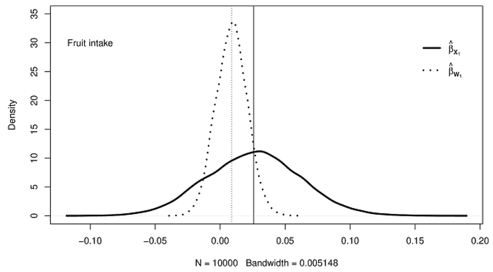
The solid vertical lines show the posterior means of coefficient estimates adjusted for bias; the dotted vertical lines indicate the posterior means of unadjusted coefficient estimates.
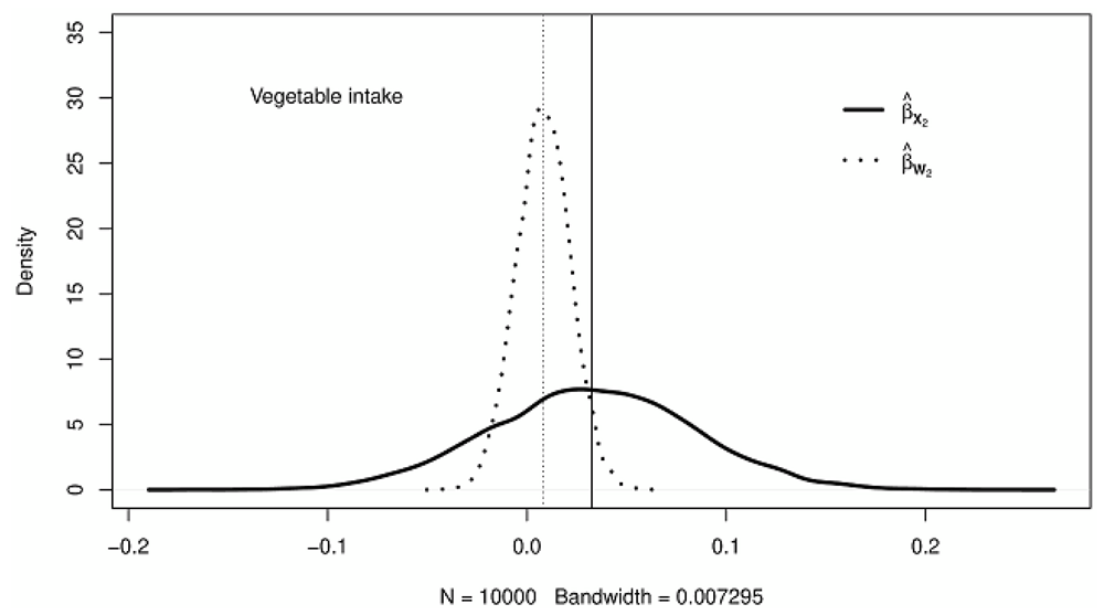
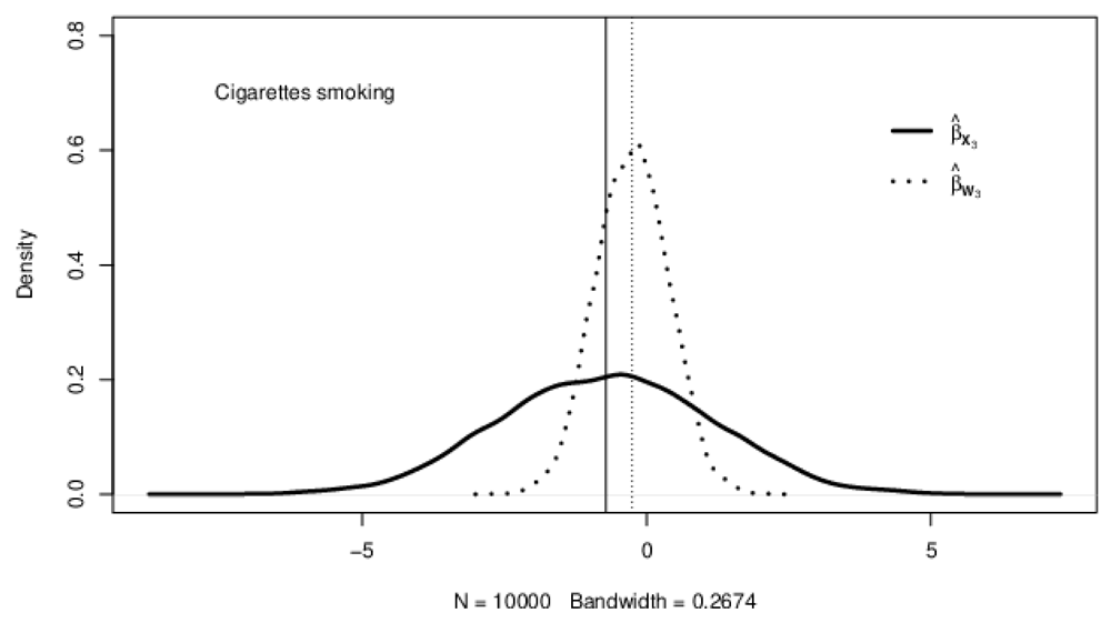
With the naive method, the variance of the regression coefficient for vegetable intake is more underestimated than for fruit intake, as depicted by the smaller length between the tails of the density plots. Of the three exposures considered in this study, the regression coefficient variance for the average number of cigarettes smoked is the most underestimated (see Table 1 and Figure 1–Figure 3). In general, a comparison of the regression coefficients’ variance in the naive and the trivariate method shows that the naive method underestimates the variance of regression coefficients.
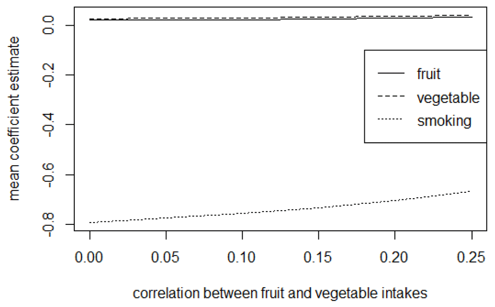
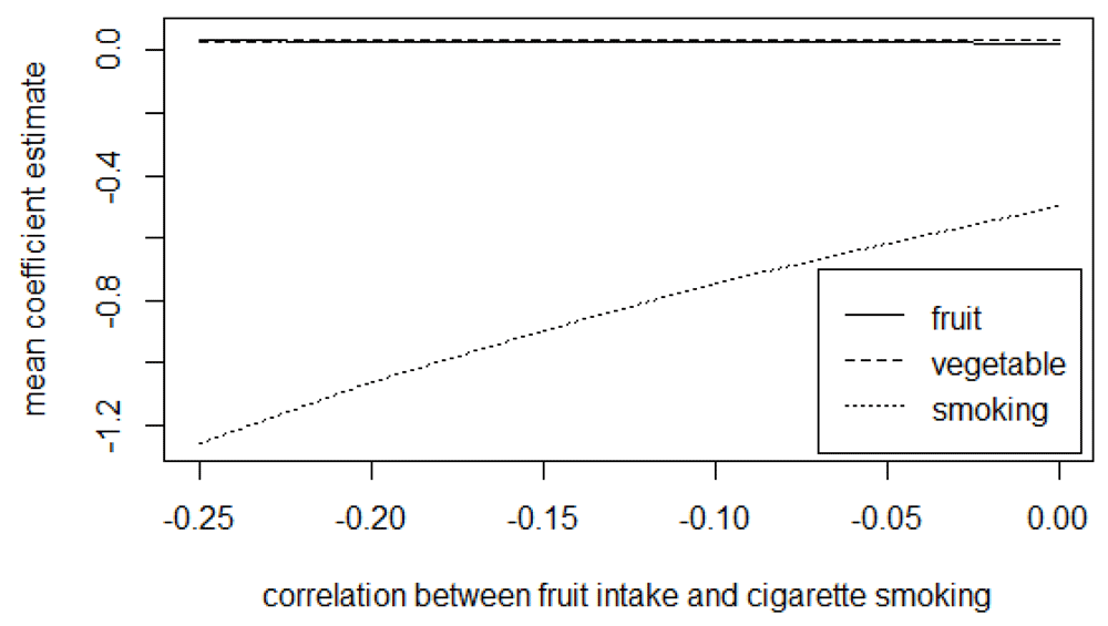
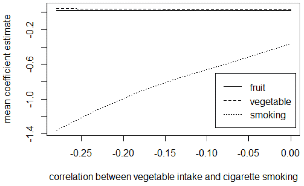
Presented in Table 2 are the mean (standard deviation) and the median for the estimates of fruit, vegetable, and the average number of cigarettes smoked adjusted for measurement error using the trivariate method in exploring the effects of the magnitude of uncertainty in the reported validity coefficients. From the results, the CI assumed in the distribution of the validity coefficient does not affect the mean and the median estimates of fruit, vegetable, and smoking. With the trivariate method, the results further show that the estimates’ uncertainty is slightly affected by the level of uncertainty assumed for the validity coefficients. Figure 4 to Figure 6 presents the mean coefficient estimates of fruit, vegetable and the average number of cigarettes smoked adjusted for measurement error using the trivariate method in the sensitivity analysis by varying the magnitude of error correlation between measurements for the exposures (see Tables D1 to D3 in the extended data for more details28).
The graphs show that varying the magnitude of the correlation between errors in any two exposures affects the estimates for the three exposures. For instance, from Figure 4, increasing the magnitude of the positive correlation between errors in fruit and vegetable intakes increase the mean estimates for both fruit and vegetable intake while it causes a decrease (in absolute value) in the estimate for the average number of cigarettes smoked; decreasing the negative correlation between errors in the measurements for fruit and cigarette smoking decreases (in absolute value) the mean estimates for both fruit and the average number of cigarettes smoked while it leads to an increase in the estimate for vegetable intake (Figure 5). Similarly, a decrease in the magnitude of the negative correlation between errors in vegetable and number of cigarettes smoked causes a decrease (in absolute value) in the estimates for both vegetables and the average number of cigarettes smoked and an increase in the estimates for fruit intake (Figure 6).
In this study, we proposed and illustrated a method that adjusts for measurement error in multiple exposures measured with correlated errors in the absence of internal validation data. The method combines external validation data from the literature with the observed self-reported data to adjust for bias in the association between the exposures and the outcome and conduct a sensitivity analysis on the measurement error and correlation between the errors. The advantages of the multivariate method presented in this work includes: (1) the method can be used to adjust for bias in the outcome-exposure association caused by measurement error reported in multiple exposures measured with correlated errors, (2) the method is useful in the absence of the costly internal validation data, provided that external information on the correlation between the observed and the true data or the error correlations of the observed data are plausible within the study context, (3) it can be used in the sensitivity analysis on the effect of uncertainty of the reported validity coefficients, (4) can be used for sensitivity analysis on the magnitude and the direction of correlated errors, (5) the method can adjust for confounding effect in the outcome regression model and (6) This method can be easily implemented on the readily available and free software R as shown in the extended data28. Often, fruit and vegetable intakes are considered as one food group. Our study is relevant because fruit intake and vegetable intake are separately assessed as independent food groups and adjusted for correlated measurement errors.
In the HBCT study example used for illustration, the estimates for fruit intake, vegetable intake, and the average number of cigarettes smoked adjusted for bias using the trivariate method were almost similar to the estimates adjusted for bias using the univariate method. The slight differences between the bias-adjusted coefficient estimates in the univariate and trivariate methods could be attributed to the weak correlations between errors assumed in this study. Sensitivity analysis on the magnitude of error correlation showed that the estimates obtained using the two methods would be different when stronger error correlations are assumed. Further, from the sensitivity analysis, we found that in a case where multiple exposures are measured with correlated errors, an increase in the magnitude of error correlation between two exposures can increase their estimates and decrease the estimate of the other exposure. From the sensitivity analysis of the level of uncertainty using CI assumed for the validity coefficients, we found that the assumed CI minimally influenced the exposures’ estimates. However, the CIs for the validity coefficients should be reasonably chosen as studies have shown that uncertainty in the estimates may be affected by the level of uncertainty assigned to the validity coefficients14. From our results, we also noted that the presence of measurement error in multiple exposures can bias the association in either direction.
This study has a few limitations: (1) for simplicity, we assumed that the exposures are measured without systematic bias, i.e., only with random errors. However, in practice, the exposures can be measured with systematic error. In such a case, the systematic error components can be incorporated in the measurement error model and also in estimating the attenuation-contamination matrix; (2) although we can have a multiplicative measurement error structure42, our study assumed an additive measurement error structure. Exposures measured with multiplicative error can be handled using our method by first converting the multiplicative structure to an additive structure through a suitable transformation that linearizes the error structure and (3) our study focused on a subset of current daily smokers, which is not a representative of the HBCT cohort and, therefore, the results are not generalizable.
From the findings of this study, we conclude that the multivariate method can be used to adjust for bias in the outcome-exposure association in a case where two or more exposures are measured with correlated errors. This is possible even in the absence of internal validation data provided that there is prior information about the validity of the data collection instruments and the magnitude of the measurement error correlation between the exposures. The method is useful in conducting a sensitivity analysis on the magnitude of measurement error and the sign of the error correlation.
Data used in this study are made available to the researcher upon registration and agreeing to the terms and conditions of use in the HSRC web site at http://curation.hsrc.ac.za/ Dataset-565-datafiles.phtml.
Figshare: A Method to Adjust for Measurement Error in Multiple Exposures Measured with Correlated Error in the Absence of Internal Validation Study-Supplementary materials. https://doi.org/10.6084/m9.figshare.13147970.v228
The file shows the validity coefficient derivation, Proof for the estimate of error variance, R code for implementing the methods and convergence diagnostics results (i.e. Trace plots and ACF plots for the standard deviation and naive regression coefficient estimates of the fruits, vegetables and average number of cigarettes smoked, with explanation) and the sensitivity analysis results (supporting Tables) for varying the magnitude of error correlation between the exposures.
The extended data are available under the terms of the Creative Commons Zero (CC0) license.
We thank the University of KwaZulu-Natal for providing the resources needed to conduct our research. Finally, we are grateful to HSRC for allowing us to make use of their data for illustration purpose.
| Views | Downloads | |
|---|---|---|
| F1000Research | - | - |
|
PubMed Central
Data from PMC are received and updated monthly.
|
- | - |
Is the rationale for developing the new method (or application) clearly explained?
Yes
Is the description of the method technically sound?
Yes
Are sufficient details provided to allow replication of the method development and its use by others?
Yes
If any results are presented, are all the source data underlying the results available to ensure full reproducibility?
Yes
Are the conclusions about the method and its performance adequately supported by the findings presented in the article?
Partly
Competing Interests: No competing interests were disclosed.
Reviewer Expertise: Biostatistical methods, particularly of dealing with confounding, selection bias, measurement or misclassification error and interference.
Is the rationale for developing the new method (or application) clearly explained?
Yes
Is the description of the method technically sound?
Yes
Are sufficient details provided to allow replication of the method development and its use by others?
Yes
If any results are presented, are all the source data underlying the results available to ensure full reproducibility?
Partly
Are the conclusions about the method and its performance adequately supported by the findings presented in the article?
Yes
Competing Interests: No competing interests were disclosed.
Reviewer Expertise: Biostatistics, measurement error, randomized clinical trials
Alongside their report, reviewers assign a status to the article:
| Invited Reviewers | ||
|---|---|---|
| 1 | 2 | |
|
Version 1 18 Dec 20 |
read | read |
Provide sufficient details of any financial or non-financial competing interests to enable users to assess whether your comments might lead a reasonable person to question your impartiality. Consider the following examples, but note that this is not an exhaustive list:
Sign up for content alerts and receive a weekly or monthly email with all newly published articles
Already registered? Sign in
The email address should be the one you originally registered with F1000.
You registered with F1000 via Google, so we cannot reset your password.
To sign in, please click here.
If you still need help with your Google account password, please click here.
You registered with F1000 via Facebook, so we cannot reset your password.
To sign in, please click here.
If you still need help with your Facebook account password, please click here.
If your email address is registered with us, we will email you instructions to reset your password.
If you think you should have received this email but it has not arrived, please check your spam filters and/or contact for further assistance.
Comments on this article Comments (0)