Keywords
COVID-19, SARS-CoV-2, prediction of spread, time series modelling
This article is included in the Pathogens gateway.
This article is included in the Emerging Diseases and Outbreaks gateway.
COVID-19, SARS-CoV-2, prediction of spread, time series modelling
The pandemic of coronavirus disease 2019 (COVID-19), caused by acute respiratory syndrome coronavirus 2 (SARS-CoV-2) represents the most serious public health threat during the last century.1 The global impact of COVID-19 has been profound. As of 12 September 2021, over 224 million cases and 4 million deaths have been confirmed globally.2 Forecasting the imminent spread of COVID-19 informs policymaking and enables an evidence-based allocation of medical resources, arrangement of production activities and economic development.3 Therefore, it is urgent to establish efficient trend prediction models, on the latest available data, to provide a point of reference for the governments to formulate adaptive responses based on reliable predictions on the impending progress of the pandemic.
The classical Susceptible-[Exposed]-Infected-Recovered (SEIR/SIR) epidemic models,4 have been widely developed to simulate the transmission dynamics of COVID-195,6 and the impact of non-therapeutic interventions – e.g., travel and border restrictions,7,8 quarantines and isolations,5,9–11 or social distancing and closure of facilities – on the spread of the pandemic, and in some cases, on the healthcare demand.5,9,11–13 These studies have been mostly focused on calibrating models for a specific country/region based on the data at the time of the model-development and assuming a multitude of parameters initialized upon prior knowledge such as social contact structure, rate of compliance with the policy and incubation or infection period among others. Complementing upon SEIR mathematical models, and owing to the increased amount of data and consistency of reports, some recent efforts have been focused on developing statistical3,14 or machine learning methods15 to predict the near-future spread of COVID-19 (in terms of the number of confirmed cases or deaths) based on the historical data.
While reliable predictions of the pandemic trend are essential for policymaking and resource-allocation, there is a lack of an adaptive real-time modelling platform which evolves as new data arrives. Here, we present, COVIDSpread, a time-series online platform for real-time modelling of the progression of COVID-19 using the Autoregressive Integrated Moving Average (ARIMA)16 statistical analyses combined with different non-linear transformation approaches.17 Our platform offers an interactive online dashboard which efficiently generates country-wise predictive models, in real-time, based on the latest report of COVID-19 cases worldwide.
The proposed modelling approach neither relies on strict modelling assumptions (e.g., linearity, stationarity, or existence of an epidemic steady state) nor on any initial parameters requiring a priori knowledge. It offers a transparent mathematical function to better understand the trend and to predict future points in the series. Different types of transformation have been examined to capture the nonlinearity in the time-series data followed by multiple differencing steps to eliminate the non-stationarity status.
The main objective of this study is to introduce an easy-to-use and readily available statistical tool to develop rigor models for time series data of COVID-19 as data becomes available on a real time basis. In this article, it is demonstrated that the proposed modelling tool is reliable to estimate accurate model parameters and predict the short-term spread of COVID-19 across different countries.
The structure of the data and the autocorrelation between daily reported instances makes an intuitive case for time series analyses. Autocorrelation occurs when there is a correlation between ordered observations in time or space resulting in the covariance between the error terms being nonzero. In the context of the ordinary least square method, where the dependent variable (even if it is observed for multiple times) is regressed only against the explanatory variables rather than previous observation of the dependent variable, the estimated parameters remain unbiased (their expected value is equal to the true values), and asymptotically normally distributed. However, the coefficients are not any-more efficient (not having the minimum variance) which means that, the commonly used, t and F statistics are not any more reliable.
If we define as the dependent variable, i.e., the number of confirmed cases, and as the explanatory variables, i.e., an intervention, being a parameter to be estimated, and as the residual at time t; in a typical linear regression models, we have which can be simply written as for one time interval earlier than t. This can be extended for s time intervals earlier as . To examine the first order autocorrelation (s = 1, i.e., only the correlation between residuals are considered which can be simply translated to the dependency between and ), the unobserved part of the error terms are correlated and denoted by , where is white noise series and can be estimated which is the main factor for examining the strength of autocorrelation as well as correcting the estimated coefficients.
Time series models implicitly assume that the stochastic process is stationary which loosely implies that mean and variance of data do not change over time. Then by using autoregressive regression (AR, as explained in the previous paragraph) and a moving average (MA, as explained in the next paragraph) mechanism, unbiased parameters can be estimated. If the data is not stationary, there are ways to transform it to stationary data such as by differencing i times which is denoted as I(i), integrated of order i.
When is defined for one side, i.e., dependent on the past, and it is weighted by parameters, say for the earlier time intervals), a moving average model is constructed as:
where . In this case, is observed and is estimated. The main difference between MA and the AR model is that several instances of white noise appear on the right-hand side of MA while past instances of the dependent variable do not appear on the right-hand side of the MA equation. In other words, in the MA model white noise of previous time intervals is scaled and carried over to the later time intervals while captures a drift in the number of cases in each time interval.When the data includes both the impact of scaled white noise and previous instances of the dependent variable affecting the current situation and ARIMA model is used. Unlike the compartmental models in epidemiology (e.g., SIR/SIER), ARIMA does not require exogeneous information about the susceptible population and recovery patterns. Instead, it captures the declining or increasing pattern of the data by extracting information from the nonlinear trends observed in the previous time intervals.
The platform retrieves daily number of confirmed cases from Coronavirus Resource Centre at John Hopkins University using coronavirus R package. Yet, it is independent of data source and can incorporate other major COVID-19 reporting parties (on countries, provinces and territories time-series), and can be readily extended to model number of deaths or recovered cases. John Hopkins reports latest available public data on COVID-19 on daily bases for all affected countries; latest data can be directly accessed from R environment. Countries with more than 30 reporting days from >50 cases were retained by the dashboard assuming that filtered countries do not hold enough data for reliable modelling/forecasting. At the time of submission 195 counties pass this constraint and modelled by COVIDSpread. The number of countries modelled increases continuously, as number of observations increases daily.
The data driven approach of this study employs three transformation operations including Ratio transformation (the ratio of observations in two consecutive days), power transformation (nth root) and logarithmic (natural log) transformation to stabilize variance in raw data and adjust the historical data for a simpler forecasting task. Models on transformed data were compared against the models developed for the non-transformed data and the best overall model were selected.
Time series models often assume stationary time-series which implies that statistical properties such as mean, variance, autocorrelation, etc. are constant over time Other than transformation, differencing once or twice (i.e., differencing between the values of consecutive data points) helps estimating the speed of growth or the acceleration/deceleration of growth. If data is non-stationary based on augmented Dickey–Fuller (ADF) test, the differencing step were applied one or more times to eliminate the non-stationarity (ADF p-value > 0.05). The differencing step allows to develop a model that is comparable to models developed based on in the SIR\SIER models. The differencing will continue until the stationary status is obtained.
Once stationary data is obtained, the best ARIMA (p, i, q) model were fitted to each time-series by searching through different combinations of p which is the order of the autoregressive model, i is the degree of differencing (as previously discussed), and q is the order of the moving-average model. The ‘auto.arima’ function in the R ‘forecast’ package has been used for model optimisation using non-stepwise selection. The selection of the best model is based on the root mean square error (RMSE) value estimated based on an out of sample estimation process on the latest 20% part of the observations (as a rough estimate of out-sample RMSE). The best model would be then used for prediction of the disease spread in the next N days (defined by the user) using the parameters of the model. The developed models can be then used to forecast changes in the number of infected cases. The prediction algorithm simulates the expected total number of infected cases as well as a bandwidth around the expected values reflecting the 80%-95% confidence level which is estimated based on the significance of the estimated parameters.
The whole pipeline including automated data retrieval, pre-processing and modelling, has been implemented in R, providing a unified platform for ease of reuse and maintenance. The online dashboard has been developed using R Shiny. Scheduled data updates were automated via a reactive file reader. Interactive line plots and maps were visualised using R-integrated Plotly and Leaflet JavaScript graphing libraries, respectively. We recommend clearing the browser autocomplete history to delete previous selections from the date-picker. The shiny web server can run in any modern web browser including Google Chrome, Mozilla Firefox, and Safari. Moreover, the COVIDSpread source code can be run using the RStudio IDE on a standard workstation (Windows/Linux/Mac) with an i5 processor and 8 GB RAM.
Multiple transformation operations are investigated to stabilise variance, coupled with recursive differencing until eliminating non-stationarity in the time-series data, i.e., p-value < 0.05 based on augmented Dickey–Fuller test.16 Upon each transformation, the best ARIMA model is obtained for each country, according to Akaike information criterion (AIC) value using maximum likelihood estimation. The optimal model for each transformation is then recorded based on the overall model Root Mean Square Error (RMSE) on the last 20% of observations reported as a surrogate estimate of out-sample prediction performance where models are trained on the first 80% of data. The predictive power of the best model per country is compared against estimations provided through exponential growth in number of cases including, 1) doubling time of two days, 2) doubling time of three days and 3) doubling time of one week, as well as a conventional linear univariate regression on log-transformed data. Extended Table 1 shows the parameters of the optimal ARIMA model per country and the corresponding RMSE measures (of the last 20% of observations) compared with conventional trends using data obtained on 23rd April 2021 from Coronavirus Resource Centre at John Hopkins University (https://coronavirus.jhu.edu). While, the purpose of this study is not to develop the most accurate time-series predictive model, statistics of the Extended Table (Extended Table 1 shows that using a more sophisticated statistical model significantly improves the prediction accuracy of COVID-19 spread in the near future (Wilcoxon test p-value << 0.001 comparing distributions of residuals).
Different time-series transformation operations, namely power transformation, logarithmic transformation and ratio transformation, have been applied to pre-process the data prior to the differencing step. We have observed that the type of transformation can significantly improve the performance of a model (in terms of the estimated out-sample RSME) as there is no a priori knowledge about the best-performing transformation (except that power transformation always performs poorly). Figure 1 shows some countries, as case studies, whose ARIMA models (as of April 23, 2021) are significantly affected by the type of transformation. As Figure 1 shows models on countries such as Zimbawe and Burundi has better performance with logarithmic transformation. For Nepal, Argentina and Greece, ratio transformations provide superior results. The case of Eswatini, interestingly, demonstrates that the ratio and logarithmic transformations outperform without transformation because the model can capture rapid fluctuation better with those transformations. Overall, the results signify the value of a performance-driven transformation selection approach upon trying multiple operations, as implemented in this platform.

Six countries were selected as case studies to demonstrate the effect of ratio and logarithmic transformations on the model performance as measured by RMSE on last (most recent) 20% of time-series data. The solid line shows the observed trend and the dashed lines shows model fitted values without transformation (red) and after ratio (green) or logarithmic (blue) transformation. The bar plot beside each trend graph shows the corresponding RMSE estimations.
The nonlinear dynamic system underlying COVID-19 spread is producing a regularly disrupted pattern making static predictions increasingly unreliable. Accordingly, a powerful feature of the platform is dynamic model estimation, that is, all models are re-optimised temporally with availability of new daily observations. Accordingly, the latest reports on COVID-19 case numbers are reflected in model estimation which accounts for the impact of new interventions improving the reliability of the future forecasts. As a case study, we have chosen to show the value of this feature on prediction of future case numbers in Iran. Iran’s trend shows significant fluctuations in the last 10 days (as of April 13, 2020) offering an interesting case study. We assumed that the model has access to data up to April 03, and then reported the next 10 days predictions and the RMSE of predicted number on April 13th. This procedure was repeated 9 times, where new observations became available to the model, one at the time. Figure 2 shows how such dynamic re-estimation adjusts the model with emerging pattern in time-series trend and improves prediction accuracy.
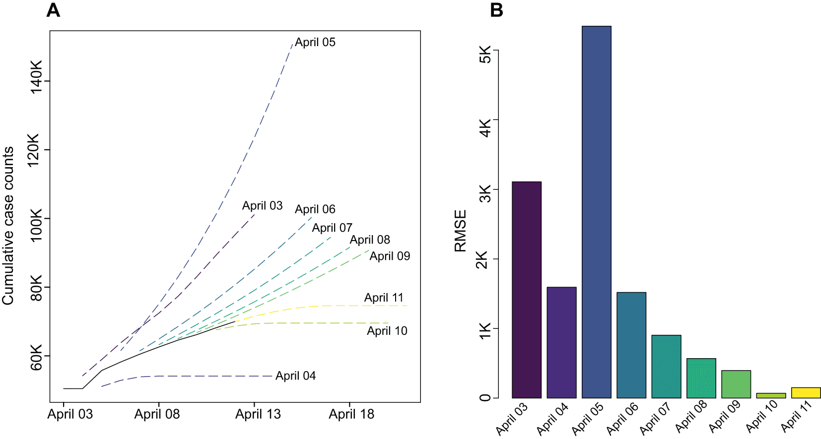
A. Predictions of next 10 days for COVID trend in Iran, assuming that the last available date was April 03 2020 to April 11 2020 as marked on the plot (last obsereved date at the time of analysis: April 13). Solid line shows observed cases. B. RMSE comparing predictions with obsereved data at April 13.
We have developed an interactive online dashboard to facilitate real-time model development for lay users as well as data scientists (Figure 3). Users can select the country of interest from the left panel and observe an interactive visualisation on cumulative counts of confirmed cases in the middle panel. Upon pressing the ‘Predict’ button’, the platform provides users with optimal models fitted to the latest reports of COVID-19 spared as provided by John Hopkins University Coronavirus Resource Centre. For any country of interest, the interactive user-interface enables users to re-estimate models by customising the range of days to be included in the model. The right panel visualises the cumulative number of confirmed cases since the 1000th case of top 10 countries in terms of total number of cases, plus predictions of growth trajectories in the next 10 days. Similarly, the middle-button panel shows the world map color-coded with predicted number of cases per 100K, together providing a global comparative view of the forthcoming COVID-19 spread. The dashboard back-end, i.e., data mining, pre-processing, and model development were implemented in R with several R packages including forecast, tseries, tsir, imputeTS, and coronavirus. The front-end of the dashboard was implemented in R shiny with several R packages, including rplotly, ggplot2, ggiraph, leaflet, DT, sparkline, data.table, survival, tidyr, and shinyWidgets. Having a single codebase for the whole framework is useful, especially in the context of reproducibility and ongoing maintenance. This dashboard offers users to not only view information in an interactive manner (e.g., on mouse hover), but also allows to download the parameters of the selected model used for the forecasting.

Real-time COVID-19 data analytics have been mainly focused on visualizing the spread18 with comparatively less effort in developing models to dynamically analyze the data. Epidemiological models, i.e., SIR/SIER models, have a strong foundation in analyzing epidemic growth/decline, and have been substantially explored for modelling the speed of infectious disease progression. Yet, such models are often offline/static, require assumptions for the parametric formulation of the model and rely on multitude of initial parameters.
Aside from SIR/SIER models, several models have been used to predict COVID-19 cases, including ARIMA, nonlinear autoregression neural network (NARNN), support vector regression (SVR), Prophet, and different deep neural network-based models such as long short-term memory (LSTM)/Stacked LSTM, Convolutional LSTM, and Bidirectional LSTM.
Tomar and Gupta19 and Chimmula and Zhang20 are two recent studies that concentrate on the LSTM model. In a similar vein, Shastri, et al.21 developed LSTM, Stacked LSTM, Bidirectional LSTM, and Convolutional LSTM models for COVID-19 cases prediction. Another area of study is the use of a recurrent neural network (RNN) to predict possible COVID-19 cases which was followed by Arora, et al.22 with proposed models based on RNN, LSTM, Bi-LSTM. Similarly, Hawas23 used RNN for daily COVID-19 infection predictions.
Aside from LSTM and RNN, one of the most commonly used models is the ARIMA time series model. Several studies focused on ARIMA models for predicting future cases including Alzahrani, et al.24 with forecasting the spread of COVID-19 cases based on the ARIMA model and Shahid, et al.25 focusing on ARIMA, SVR, LSTM and Bi-LSTM models.
Along the same vein, Ribeiro, et al.26 compared ARIMA, cubist regression (CUBIST), random forest (RF), ridge regression (RIDGE), SVR, and stacking-ensemble learning for the prediction of COVID-19 cumulative cases. Similarly, Kırbaş, et al.27 focused on ARIMA, nonlinear autoregression neural network (NARNN) and LSTM for future case prediction. Likewise, Papastefanopoulos, et al.28 provided a comparison on six different forecasting methods including ARIMA, the Holt-Winters additive model (HWAAS), TBAT, Facebook’s Prophet and deep AR for active case prediction and Devaraj, et al.29 evaluated ARIMA, LSTM and SLSTM for COVID-19 prediction.
We developed a time-series based statistical model to dynamically predict the future trend of COVD-19 spread. It is coupled with the capacity of time-series models in 1) considering higher orders of derivatives of the number of cases in previous time intervals, 2) accounting for the impact of residuals of the previous time intervals. The literature demonstrates a diverse set of short-term forecasting models, although the focus of this research is on ARIMA models, other models may be considered if the developed model does not perform adequately. For example, as shown by the results, ARIMA (0,2,0) was the best-fitting ARIMA model for India, with high RMSE values. This means that the model does not include any autoregressive or moving average terms and does not provide a suitable representative of COVID-19 cases in India at the investigated time period.
Different models for analyzing COVID-spread in India can be used as an alternative as several studies have been conducted to model COVID-19 spread in India using other models. For instance, Tomar and Gupta19 used the LSTM model and Arti and Bhatnagar30 proposed a tree-based model to model spread the disease in the community. Bherwani, et al.31 used the SEIR model to model the spread of COVID-19 while Mahajan, et al.32 used the compartmental epidemic model SIPHERD for modelling spread COVID-19 cases in India. In the same line, Roy and Roy Bhattacharya33 proposed A mathematical model based on a differential equation to demonstrate how the number of asymptomatic patients grows over time and Kumari, et al.34 proposed multiple linear regression with autoregression used to predict the possible number of cases in the future.
Similarly, models based on countries like Brazil and Italy do not work well with high RMSE values, meaning that other models can be used instead. Other studies with focus on Brazil used models such as SIR,35 Holt36 and artificial intelligence (AI) models.37 Studies on Italy focused on extended SIR (eSIR) models38 and mathematical models with a Gaussian error function type.39
As shown in the results, ARIMA (5,2,5) was the best-fitting ARIMA model for Panama, Iran, and Spain when data was not transformed. Despite having the same model structure, the established model for Panama outperforms Iran and Spain with a lower RMSE values. The explanation may be due to a fluctuation in the number of cases in Iran, such as the rapid spread of COVID-19 in Iran at the start of the pandemic, and misunderstandings that led to ignoring the issue of social distance while eliminating travel restrictions one by one in April 2020 resulting in the reappearance of the virus.40 Another reason may be that the Iran COVID-19 data behavior is more complicated due to the geographical correlation of cases in Iran41 and the variation caused by sudden rises in the number of cases in different parts of the country at different times.
Another reason for the models’ disparities in performance could be the effect of weather factors on COVID-19 cases, which is being investigated by Fernández-Ahúja and Martínez.42 While Panama has a tropical maritime climate, Spain is home to four distinct climates. Climate variables clarify some key aspects of COVID-19 spread in Spain42 that are not captured by ARIMA models, whereas the influence of such variables in Panama will be less due to more consistent weather. In the same line, Gupta, et al.43 investigated the impact of weather on COVID-19 spread in the United States, while the derived model for the United States of America has a high RMSE value. Other models has been used for Iran such as LSTM,44 Recursive-based prediction model, Boltzmann function-based prediction model and Beesham’s prediction model.45 LSTM46 and SEIR47 have been employed to model the cases in USA and Spain.
While the developed model works well in African countries like Uganda, Congo, and Algeria, the model for South Africa has a high RMSE value, indicating that different models should be used for this country which is investigated by Ding, et al.48 with SIR model and Reddy, et al.49 with a set of nonlinear growth models and Nadim and Chattopadhyay50 with mathematical model considering the imperfect lockdown effect. Similarly, the developed model for Ethiopia shows high RMSE value. Other studies researched on COVID-19 cases in Ethiopia with machine learning algorithms51 and mathematical models based on susceptible, exposed, symptomatically infected, asymptomatically infected, hospitalized and recovered/immune compartments.52
As results show, developing models for a number of countries, including China and Eswatini, performs better on transformed results. Both countries have seen a rapid fluctuation in the number of cases, which can be due to a change in how the virus is diagnosed and the number of diagnostic tests conducted. While data transformation in ARIMA models can help to improve model performance by removing skewness and fluctuation from the original data, other data processing methods such as machine learning can be used for data preprotein as discussed by Pinter, et al.53 to improve the performance of models such as SIR models. In the same line, Other models for predicting new cases in China and Brazil that are developing AI and data-driven models include a data pre-processing phase.54,55 Table 1 summarises the section and the studies conducted on countries where the developed ARIMA model does not provide adequate performance.
| Country | Alternative models used in literature |
|---|---|
| India | LSTM model,19 Tree-based model,30 SEIR model,31 Compartmental epidemic SIPHERD model,32 Mathematical model based on a differential equation,33 Multiple linear regression with autoregression34 |
| Brazil | SIR model,35 Holt model,36 Artificial intelligence (AI) models,37 Data driven models54 |
| Italy | extended SIR (eSIR) model,38 Mathematical models with Gauss error function type39 |
| Iran | LSTM model,44 Recursive-Based prediction model, Boltzmann function-based prediction model, Beesham’s prediction model45 |
| Spain | LSTM model,46 SEIR model47 |
| United states | LSTM model,46 SEIR model47 |
| South Africa | SIR model,48 Nonlinear growth models,49 Mathematical model considering the imperfect lockdown effect50 |
| China | Hybrid AI model55 |
| Ethiopia | Machine learning models,51 Mathematical model based on compartmental approach of susceptible, exposed, symptomatically infected, asymptomatically infected, hospitalized and recovered/immune compartments52 |
In this study, we presented an automated modelling platform that delves into multiple layers of information in the COVID-19 time series data to find the best fit with the aim of providing robust forecasts. COVIDSpread was shown to be effective in estimating the trend of the pandemic for each country. We elaborated the importance of data transformation as a preprocessing step and shown that there is no transformation operation which consistently provides the best fit to the data. Hence, exploring multiple options are recommended to stabilize variations prior to modelling using conventional econometrics formulations. A unique aspect of the presented platform is that it facilitates real-time model development incorporating latest reported data into modelling. We have shown that such adaptive model estimation significantly improves the prediction power and therefore, forecasting reliability.
The platform retrieves daily number of confirmed cases from Coronavirus Resource Centre at John Hopkins University using coronavirus R package.
Zenodo: VafaeeLab/COVIDSpread: First release of COVIDSpread, https://doi.org/10.5281/zenodo.5587835.56
This project contains the following extended data:
COVIDSpread is available online: http://vafaeelab.com/COVID19TS.html
All the codes, including Shiny app is available at the project GitHub Repository: https://github.com/VafaeeLab/COVIDSpread
Archived code as at time of publication: https://doi.org/10.5281/zenodo.558783556
License: Apache License, Version 2.0
| Views | Downloads | |
|---|---|---|
| F1000Research | - | - |
|
PubMed Central
Data from PMC are received and updated monthly.
|
- | - |
Provide sufficient details of any financial or non-financial competing interests to enable users to assess whether your comments might lead a reasonable person to question your impartiality. Consider the following examples, but note that this is not an exhaustive list:
Sign up for content alerts and receive a weekly or monthly email with all newly published articles
Already registered? Sign in
The email address should be the one you originally registered with F1000.
You registered with F1000 via Google, so we cannot reset your password.
To sign in, please click here.
If you still need help with your Google account password, please click here.
You registered with F1000 via Facebook, so we cannot reset your password.
To sign in, please click here.
If you still need help with your Facebook account password, please click here.
If your email address is registered with us, we will email you instructions to reset your password.
If you think you should have received this email but it has not arrived, please check your spam filters and/or contact for further assistance.
Comments on this article Comments (0)