Spatio-temporal characteristics of Tuberculosis in Ghana

TB cases

In this study TB detection data obtained from Ghana Health Service and National Tuberculosis Programme was used.⁸ The data contained information on TB detection from 2009 to 2017, for the 10 old administrative regions of Ghana. These regions include, Ashanti, Brong Ahafo, Central, Eastern, Greater Accra, Northern, Upper East, Upper West, Volta, and Western.

Figure 1 shows the TB trends in the 10 regions from 2008 to 2017. Generally, there is a decrease in TB cases observed in all regions (except Brong Ahafo Region where TB cases increase) of Ghana from 2008 to 2016. It can also be observed that TB cases in Northern and Upper East increased remarkably between 2016 and 2017, whereas cases in Ashanti Region decreased from 50 per 100, 000 population in 2016 to 45 per 100,000 population in 2017. In the Northern Region, TB cases increased from 24 per 100,000 population in 2016 to 52 per 100,000 population in 2017. Further, cases in Upper East Region increased from 53 per 100,000 population in 2016 to 63 per 100,000 population in 2017. However, the changes in TB cases in the other regions are almost horizontal.

Figure 1. Trend of TB cases detection per 100,000 by region for 10 years from 2008 to 2017 in Ghana.

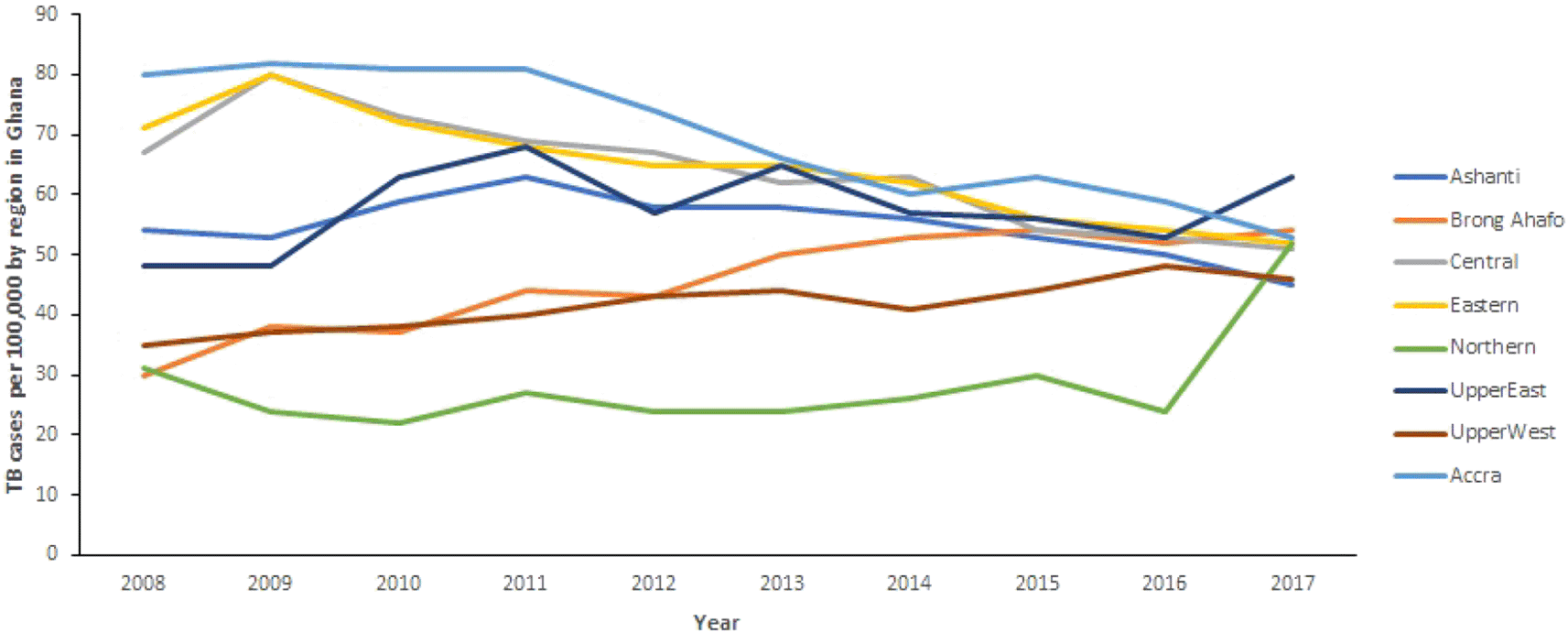
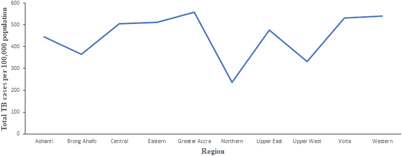
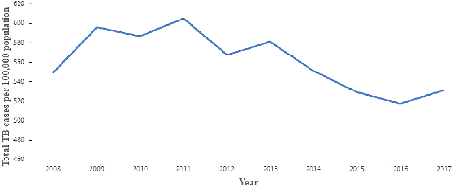
Figure 2 shows the trend of total number of TB cases for each region from 2008 to 2017. It shows that the highest cases recorded was in the Greater Accra Region from 2008 to 2017. It also shows that the lowest was recorded in the Northern Region. Volta and Western Regions are second and third, respectively, with records slightly lower than Greater Accra Region. In addition, Figure 3 shows the trend of total TB cases in each year/period. The figure shows that the highest number of total TB cases was recorded in 2011 while the lowest was in 2016. It can be observed that TB cases decreased slowly from 2011 to 2017 with increments in 2012 and 2017.

Figure 2. Trend of the total TB cases detection per 100,000 for each region from 2008 to 2017 in Ghana.

Figure 3. Trend of the total TB cases detection per 100,000 population for each year.

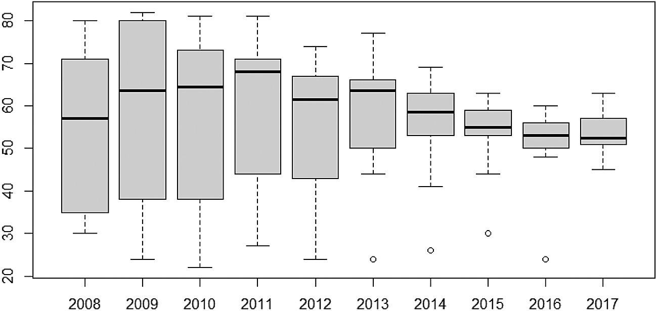
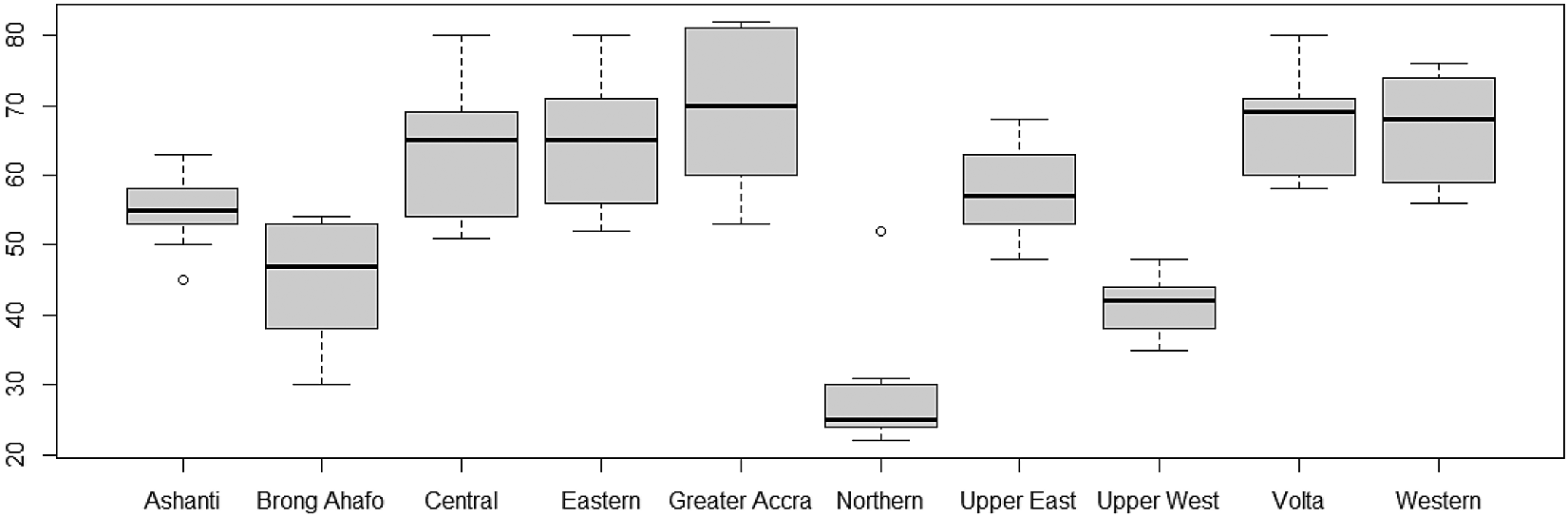
Furthermore, the variability of TB cases from 2008 to 2017 have also been presented using box-and-whisker plots in Figure 4. The overlapping box-and-whisker plots imply that there is no variability in cases among the years. The plots show that TB cases were skewed towards larger numbers from the year 2008 to 2014, and skewed towards smaller numbers from 2015 to 2016. Extremely small numbers were observed in 2013, 2014, 2015, and 2017. Variability across the regions have been presented in Figure 5. None-overlap of box-and-whisker plots imply variability between regions. Thus, there is variability in TB cases among the regions since some of the box-and-whisker plots do not overlap. It can also be observed that TB cases in most of the regions are skewed towards larger numbers except Northern and Upper East Regions (especially, the Northern Region with one extremely large value).

Figure 4. Box-and-whisker plot of TB cases detection per 100,000 population for each year.

Figure 5. Box-and-whisker plot of TB cases detection per 100,000 population by the 10 old administrative Regions in Ghana.

Baseline predictors

Some baseline regional characteristics on the risk of TB infection have been explored in this study. The set of baseline predictors include doctor to population ratio, nurse to population ratio, HIV prevalence, TB cure rate, TB success rate, wealth quantiles and the proportions of men/women employed, unemployed, educated, and uneducated. Variables also considered in the study include proportions of people who have heard about the TB disease, have knowledge that TB is airborne, knowledge that TB can be cured, and those who believe that TB status should be kept secret. In the data analyses, all the baseline variables were explored to obtain significant predictors of the TB cases.

Hierarchical space model

For spatial TB data, let $y_i,i=1,\dots ,n$ denote a Poisson random variable with probability mass function defined as $P\left(y_i|\mathit{\theta }\right)$, where $\mathit{\theta }=\left({\theta }_1,\dots ,{\theta }_n\right)$ is a vector of relative risk parameters for each region. The variable $y_i$ represent total number of TB cases for region $i.$ It follows that the likelihood function for the Poisson variable $y_i$ is defined as:

Moreover, after covariate adjustments, statistical inferences remained unchanged and the classical parametric formulation (in Equation 7) remains the most accurate model for the TB data. The posterior summary statistics in Table 6 showed negligible risk of TB across the 10 regions. Precisions of both the unstructured and structured components indicate clustering of risk. The models are implemented in R-software via the Integrated Nested Laplace Approach (INLA) packagon. Instructions on downloading and how to use this package can be found in Håvard et al.²⁰ Also, this package can directly be installed in R software by using the command install.packages("INLA",repos=c (getOption("repos"),INLA="https://inla.r-inla-download.org/R/stable"), dep=TRUE).

Correlated and uncorrelated heterogeneity structures

The clustering and variability of risk were studied using correlated and uncorrelated structures, respectively. The use of uncorrelated heterogeneity models with gamma or beta prior distributions for estimating the relative risk of a given disease are useful, however, such models have limitations. Andrew [17, P. 82-84] stated that a gamma distributions restrict the incorporation of covariates into the modeling process. Another limitation is that such models do not allow the formulation of a simple and adaptable general form of the gamma distribution with spatially correlated parameters [17, P. 82-84]. Wolpert and Ickstadt²¹ have also given an example of correlated gamma field models that yield poor results.²² However, Gaussian models permit incorporation of correlated structure (CH) into the modeling process. Further, variability in the data can be modeled as uncorrelated heterogeneity (UH) using a Gaussian prior distribution with a mean zero and risk variance of the disease across the regions. Both correlated and uncorrelated heterogeneity can be incorporated into the model to account for clustering and heterogeneity of risk. These structures are introduced into the modeling through a log-linear term with additive random effects.^18,23 Besag et al.²⁴ have provided the form of the model with CH and UH structures parameterized as follows:

Conditional Auto-regressive (CAR) models

CAR models provide a tool for detecting and identifying regions where disease risks are clustered. The specification of CAR models provide a framework for borrowing strength between neighboring regions in such a way that, regions that share boundaries are likely to have similar risks and regions that are distant apart are likely to show variability with regard to risk. Waldo Tobler’s²⁵ noted that “everything is related to everything else but near-by things are more related than distant things”. CAR models were rarely used to detect and cluster risk until the 1990s.^13,26 The models enable the influence of disease risk in neighboring regions to be modeled and estimated.^18,19,27 Distances or boundaries between the regions are used to determine neighborhood properties in the CAR models.^14,17,28

Let $\mathrm{\Omega }=\left\{1,2,\dots ,n\right\}$ denote the study area and $N_i=\left\{j\in \mathrm{\Omega }:i\in j\right\}$ classifies regions that share boundaries with region $i.$ Let ${\varphi }_i,i\in \mathrm{\Omega }$ be a stochastic variable, then the CH structure of ${\varphi }_i$ follows a normal distribution defined as:

Assume that region $i$ has $M$ neighbors and $W_{\mathit{ij}}=\frac{1}{M}$ for each region that is a neighbor but zero elsewhere. The conditional expectation of ${\varphi }_i$ is given by:

The Gaussian processes are defined by mean and covariance functions.³⁰ Thus, the mean and variance-covariance functions are required to specify the CAR model. It follows the conditional probability distribution of the CAR structure ${\varphi }_i$ is defined as^22,24,25:

The symmetry of $\mathrm{\Sigma }$ implies that the covariance matrix ${\mathrm{\Sigma }}^{-1}\mathrm{B}={\mathrm{B}}^{-1}\mathrm{\Sigma }$ is symmetric such that $W_{\left(\mathit{ij}\right)}{\tau }_j^2=W_{\left(\mathit{ji}\right)}{\tau }_i^2,i,j\in S.$ The probability distribution Function (3) can alternatively be defined as:

It has been proved that the CAR structure ${\varphi }_i$ follows the Gaussian distribution by showing that $\mathrm{\Sigma }$ is symmetric, see^18,31 for details.

0.0.1. Parameter estimation: CAR model

Parameters in the CAR model are estimated using Bayesian hierarchical methods. The TB detection data used in the study are counts (whole numbers), therefore, Poisson distribution is assumed for such data. The unknown risk of TB in any region $i$ represented by ${\varphi }_i.$ The number of cases and population risk in any region $i$ are denoted by $y_i$ and $N_i,$ respectively. The expected number of cases in region $i$ can then be written as:

gescrepresents the overall risk in the study population. The corresponding likelihood function is defined as:

Taking natural logarithm of the likelihood function, differentiating with respect to the disease risk ${\theta }_i$ and equating to zero, it can be shown that the maximum likelihood estimator ${\widehat{\theta }}_i$ of ${\theta }_i$ is

which defines the standardized mortality ratio (SMR) in region $i.$ However, using the Bayesian framework, $y_i\sim$ Poisson $\left(E_i{\theta }_i\right)$, where the Poisson mean ${\mu }_i=$ $E_i{\theta }_i,$ ${\theta }_i\sim$ Gamma $\left(\alpha ,\gamma \right)$ with shape parameter $\alpha$ and scale parameters $\gamma ,$ respectively. However, these formulations do not incorporate covariates in the modeling process. Covariates through a linear predictor was introduced, as seen in previous work [18, 19, 17, P. 84]. The distribution of the response variable is specified by the exponent of the linear predictor as $y_i\sim$ Poisson $\left(E_{i}exp\left({\eta }_i\right)\right)$, where ${\mu }_i=E_{i}exp\left({\eta }_i\right)$ is the mean of Poisson distribution. Thus, the relative risk of the disease in region $i$ is defined as:

Using the generalized linear model with a log-link function, we have:

Bayesian models are defined by the posterior distribution of the $\mathrm{D}$ parameter estimates, where the posterior is the product of the data likelihood function and the prior distribution(s) of the parameter estimates. Hence, we define the likelihood function as:

The $\beta$ parameter estimates are assumed to follow the Gaussian distribution defined:

The hyperprior distribution for the precision parameters ${\tau }_{\varphi }^2$ and ${\tau }_{\beta }^2$ are respectively, ${\tau }_{\varphi }^2\sim$ Gamma $\left(\mathrm{0.05,0.005}\right)$ and ${\tau }_{\beta }^2\sim$ Gamma $\left(\mathrm{0.5,0.05}\right).$ The linear regression coefficient distribution is defined by:

0.0.2 The Besag, York and Molli’e (BYM) Model

Clayton and Kaldor³³ were first to propose the BYM framework, and later, Besag et al. developed it further.²⁴ The BYM (also known as the convolution model) unifies the CH and UH structures into the same model that is capable of explaining clustering and variability of the disease risk. Although various models have been proposed for smooth risks estimation, the model proposed by Besag et al. (BYM)²⁴ have been used extensively in literature. The BYM model is expressed as follows:

As indicated in the previous section, the TB cases follow the Poisson distribution, thus, $y_i\sim$ Poisson $\left(E_{i}exp\left({\eta }_i\right)\right),$ where ${\mu }_i=E_{i}exp\left({\eta }_i\right).$ The linear link function is ${\eta }_i={\mathbf{X}}^{\prime }\beta +{\varphi }_i+u_i.$ The $log$ relative risk is $log\left({\theta }_i\right)={\eta }_i$. Therefore, the relative risk for area $i$ is defined by:

The log log-link function is defined as:

Parameter estimation: BYM

Parameters in the BYM are estimated using the same formulations discussed in the previous section, however, $u_i$ is required to be a Gaussian prior distribution given by:

The resulting posterior distribution can be written as follows:

The distributions for the hyper-prior precision parameters are as follows:

The estimates, ${\tau }_u^2$ and ${\tau }_{\varphi }^2$ are precision-variance estimates for $u$ and $\varphi ,$ respectively, and are used to measure the level of variability of risk among the regions and to cluster risk between neighboring regions.^18,27

Space-time models

The TB data used in study are collected over time and hence spatial models alone will not be enough to model the space-time pattern of the relative risk of the disease. The spatial models are constrained for identifying heterogeneity and clustering of risk at a single time point. Several methods have been proposed to account for spatial and temporal patterns of disease risks.^{23,24,34–36}

In this section, space-time models are presented based on three modeling frameworks developed by Knorr-Held et al.,^16,37 Bernardineli et al.²³ and Waller et al.³⁷ These models differ with regards to their space-time interactive structures and inclusion of covariates. Consider region $i,$ in year $t,$ that recorded $y_{\mathit{it}}$ TB cases. The cases follow the Poisson distribution, i.e.:

Our first space-time model formulations is based on the framework developed by Bernardineli et al.,²³ where the linear predictor ${\eta }_{\mathit{it}}$ is:

It follows that the Poisson mean is

These formulations suggest that each spatial unit has its own time trend with a spatial intercept $\left(\mu +{\varphi }_i+u_t\right)$ and a slope $\left(\rho +{\delta }_i\right)$. This model assumes a linear time trend in each spatial unit. The parameters to be estimated are $\phi =\left\{\rho ,\varphi ,u,\delta \right\}$ and the hyper-parameters $\psi =\left\{{\tau }_{\varphi },{\tau }_u,{\tau }_{\delta }\right\}$.

Adjusting for risk factors $X_i$ of TB cases detection, the model 6 can be written as model 7. Now the parameters to be estimated are $\phi =\left\{\beta ,\rho ,\varphi ,u,\delta \right\}$ and the hyper-parameters are $\psi =\left\{{\tau }_{\varphi },{\tau }_u,{\tau }_{\delta }\right\}$.

It is known that if ${\delta }_i<0$ the region-specific trend is less steep than the mean trend. On the other hand, ${\delta }_i>0$ implies that the region-specific trend is steeper than the mean trend. Further, ${\delta }_i\sim \mathit{\text{Normal}}\left(0,{\tau }_{\delta }\right).$

The second space-time model is based on Waller et al.³⁰ dynamic non-parametric formulation on the linear predictor:

The ${\vartheta }_t$ quantifies temporal-structure effect and it is modeled using a random walk through a neighboring structure¹⁶ defined as:

Finally ${\varphi }_t$ is specified by means of a Gaussian exchangeable prior: ${\omega }_t\sim N\left(0,{\tau }_{\omega }\right)$. Finally ${\varphi }_t$ is specified by means of a Gaussian exchangeable prior: ${\omega }_t\sim N\left(0,{\tau }_{\omega }\right)$.

The third space-time Model 10 is an extension of Model 9 that enables a space-time interaction in order to explain the difference in the time trend of TB cases. It is expressed as follows:

In this model,$\phi =\left\{\mu ,\varphi ,u,\vartheta ,\omega ,\pi \right\}$ and $\psi =\left\{{\tau }_{\varphi },{\tau }_u{\tau }_{\vartheta },{\tau }_{\omega }{\tau }_{\pi }\right\}$were estimated, where ${\pi }_{\mathit{it}}$ is interaction between ${\varphi }_i$ and $u_i.$ The model assumes that there is no interaction between ${\varphi }_i$ and ${\vartheta }_t,$ hence, ${\pi }_{\mathit{it}}\sim N\left(0,{\tau }_{\pi }\right).$ Incorporating covariates into Model 10, yields Model 11:

Hence, $\theta =\left\{\mu ,\beta ,\varphi ,u,\vartheta ,\omega ,\pi \right\}$ and $\psi =\left\{{\tau }_{\varphi },{\tau }_u{\tau }_{\vartheta },{\tau }_{\omega },{\tau }_{\pi }\right\},\mathit{\text{needtobeestimated}}.$ For the interaction term ${\pi }_{\mathit{it}}$, it is assumed that there is spatial or temporal structure on the interaction, then ${\delta }_{\mathit{it}}\sim \mathrm{N}\left(0,{\tau }_{\delta }\right)$.³⁷ In this study, all the precision parameters are assumed to follow the gamma distribution.¹⁶

Spatial BYM without covariates adjustment

In this section, BYM without covariate adjustments (defined as ${\eta }_i=\mu +{\varphi }_i+u_i.$) was implemented. The posterior estimates are presented in Table 1. The maps of the posterior mean for the region-specific relative risks ${\zeta }_i=exp\left({\varphi }_i+u_i\right)$ of presented in Figure 6a,b are used to identify regions with high risk. High risk is visualized by computing $p\left({\zeta }_i>1|y\right),$ for details see M. Blangiardo et al.¹⁶ Figure 6a shows the five of the ten regions that have high risk of TB cases. The risk profile for TB in Ghana are shown in the figure-legends. In the regional map of Ghana, the darker the region the higher the risk and vice versa. It can be observed that Upper East and Upper West Regions have the highest risk (with values in the range 1.8-3.4), followed by Volta, Western and Central Regions with risk between 1.1-1.8. The rest of the regions have low risk of TB detection, specifically, Northern and Ashanti Regions have the lowest risk (with values in the range 0.3-0.6), followed by Greater Accra and Brong Ahafo Regions with values between 0.6-0.9. The Eastern Region has normal risk (with a value in the range 1-1.1).

Figure 6. Regional distribution of posterior relative risk of TB in Ghana, using BYM.

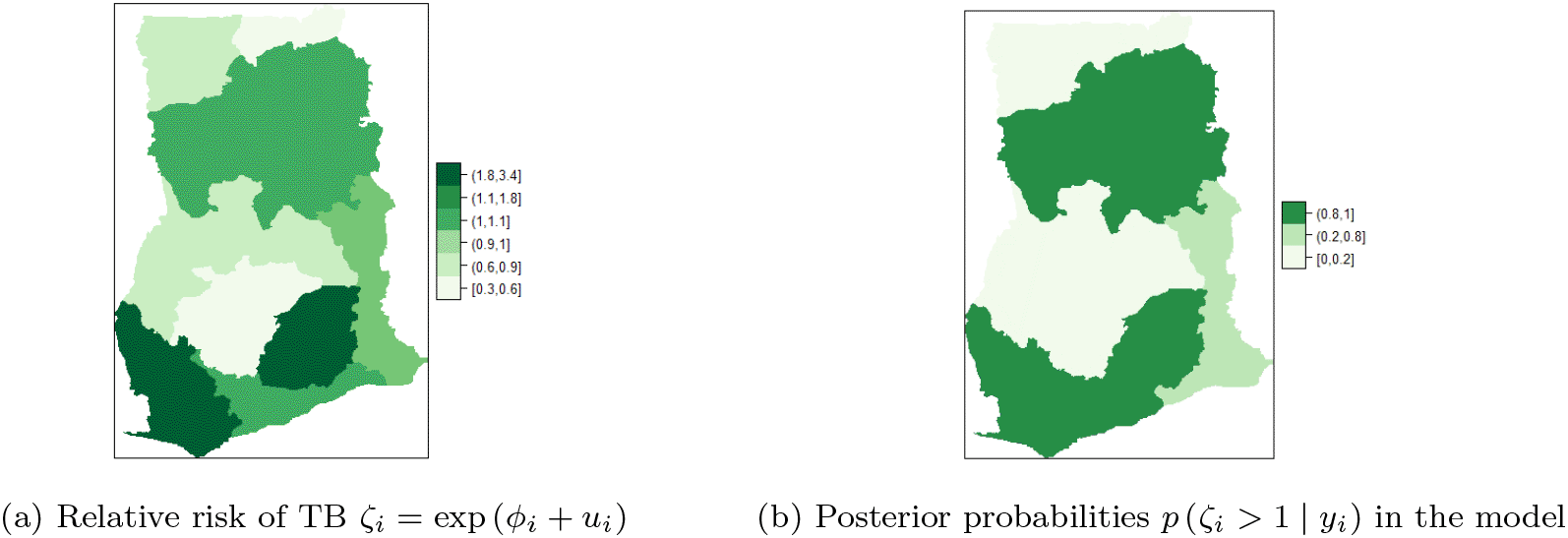
Figure 6b shows that Upper East, Upper West, Volta and Central regions have the highest posterior relative risk (0.8-1) of TB detection. The regions have similar risks, however, none of them has a risk higher than the national risk 1. Moreover, low relative risk (0-0.2) of TB detection is observed in the Northern, Brong Ahafo, Ashanti, and Greater Accra regions, followed by Eastern and Western regions that have relative risk values in the range (0.2-0.8).

The results in Table 1 confirm the similarity or clustering of risk in the neighboring regions. This is indicated by the low variability captured by the precision of the spatial structure ${\tau }_{\varphi }$. The estimate of the posterior marginal variance to capture the amount of variability explained by the spatial structure was evaluated. The spatial structure effect empirically using this formula was estimated:

The estimated proportion of spatial structure variance is approximately $10\%,$ implying that only $10\%$ of the variability is explained by the spatial structure. It further explains the remaining higher variability captured by the unstructured random effect $u_i$ component of the BYM. The precision ${\tau }_u$ of the unstructured component of the BYM model indicates that the risk is heterogeneous among regions. The exponent of the posterior mean $\mu$ (overall mean effect) shows that there is approximately a 3-fold increase in TB infections rate across the 10 regions of Ghana. The corresponding 95% credible interval ranges from $2.21$ to $4.66$.

BYM with covariate adjustments

This section represents the results obtained from experiments conducted with seven (7) covariates adjustments of the BYM:

Among the baseline predictors stated in Section b, the significant predictors for TB cases in Ghana that yield accurate models include: HIV prevalence, TB cure rate, TB success rate, proportion of people with knowledge about TB, proportion of those who know that TB is airborne, proportion in high income group and literacy. Table 2 presents posterior estimates of the overall mean, fixed effects (i.e. ${\beta }_1,\dots ,{\beta }_7$) as well as random effects (i.e. ${\tau }_u$ and ${\tau }_{\pi }$) for the unstructured and structured components of the BYM. The maps of the posterior mean for each region’s relative risk (i.e. ${\zeta }_i=exp\left({\varphi }_i+u_i+{\sum }_{p=1}^7\mathit{\beta p}\right)$) are presented in Figure 7a and b. The risk can be visualized by computing $P\left({\zeta }_i>1|y\right)$_.¹⁶

Figure 7. Regional posterior relative risk of TB in Ghana, using BYM with adjusted covariates.

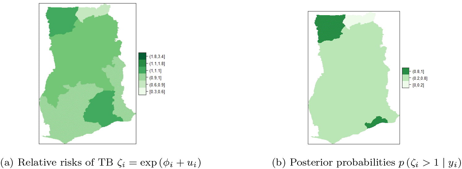
It can be observed in Figure 7a that Upper East, Brong Ahafo and Western Regions have high and similar detection risks ranging from 1.1-1.8. The adjusted risk (i.e. risk with the covariates in Figure 7a) is less than the unadjusted risk (risk without covariates in Figure 6a). Upper East Region is still among the regions with high risk of TB detection after covariates adjustment. Upper West Region does not belong to the high risk class while Brong Ahafo and Western Regions have moved to the normal risk class after the covariate adjustments. Greater Accra and Central Regions are the second highest in the high risk class, with risk ranging from 1-1.1. Upper West, Northern, Volta, and Eastern Regions are in the normal risk class, with risk ranging from 0.9-1. Further, Ashanti Region is in the low risk class (with values in the range 0.6-0.9) after covariate adjustments. In Figure 7b, it can be observed that Brong Ahafo and Western Regions have the highest and similar relative risk (0.8-1), while Ashanti Regions has the lowest relative risk (0.0-0.2). The rest of the regions have similar relative risks ranging from 0.2-0.8.

Table 2 presents the posterior estimates of fixed and random effects of the BYM with covariate adjustments. It can be observed that TB cure rate increases the risk of TB cases by approximately 8% This observation implies that as more cases are detected, more cases are cured and hence TB cases should in general decrease over time. This explains why TB success rate leads to 14% reduction in detection rates. The results also revealed that knowledge about TB significantly increases TB detection by approximately 5% This behaviour is expected because, as people become aware of TB, preventive measures are taken. High income is associated with 5% reduction in TB cases while literacy is associated with 12% increase in cases. High income increases the use of health facilities and testing for TB, thus, leading to a reduction of TB cases. HIV prevalence lead to 55% reduction in cases.

After adjusting the covariates, similarity/clustering of risk between neighboring regions, (see Figure 7) with low variability of risk among the regions was observed. This observation is captured by the precision ${\tau }_{\varphi }$ of the spatial structure in Table 2. Heterogeneity of risk across the regions has reduced after the covariates adjustment.

Furthermore, the posterior marginal variance to determine the amount of variability explained by the spatial structure using the formulations in Equation (12) was evaluated. The results showed that the estimated proportion of spatial structure variance is approximately 5%. This implies that only 5% of the variability is explained by the spatial structure. Much of the variability remaining is captured by the unstructured random effect $u_i$ component of the BYM. The precision ${\tau }_u$ of the unstructured component of the BYM indicates that risk is heterogeneous across regions.

The posterior mean of the exponent $\mu$ (overall mean effect) gives an indication that there is approximately 9-fold increase in TB infections rate across the 10 regions in Ghana.

Space-time models without covariates adjustments

Table 3 presents the DIC, mean deviance $\overline{D}$ and effective number of parameters $\mathit{pD}$ components for the three space-time models. The performance indicators show that the classical parametric formulation (see Equation (7) introduced by Bernardinelli et al.²³ is the most accurate among the three space-time models. Hence, further discussion will include only the results from that model.

The results in Table 4 show that there is about $8\%$ increase in risk of TB detection across the 10 regions of Ghana. However, this increase is statistically not significant at 5% significance level. As observed in the BYM, TB cases do not significantly increase with time. The precision parameter ${\tau }_u$ shows some level of variability in the risk of TB among the regions, while there is clustering of risk between neighboring regions exhibited by the high precision parameter ${\tau }_{\varphi }$ for the spatial structure. High precision characterized by ${\tau }_{\delta }$ indicates low variability associated with ${\delta }_i.$ This further indicates that there is less interaction between space and time, as well as global trend $\rho$ and areas-specific trend ${\delta }_i.$ Hence, the area-specific trend ${\delta }_i$ is less remarked than the mean trend.

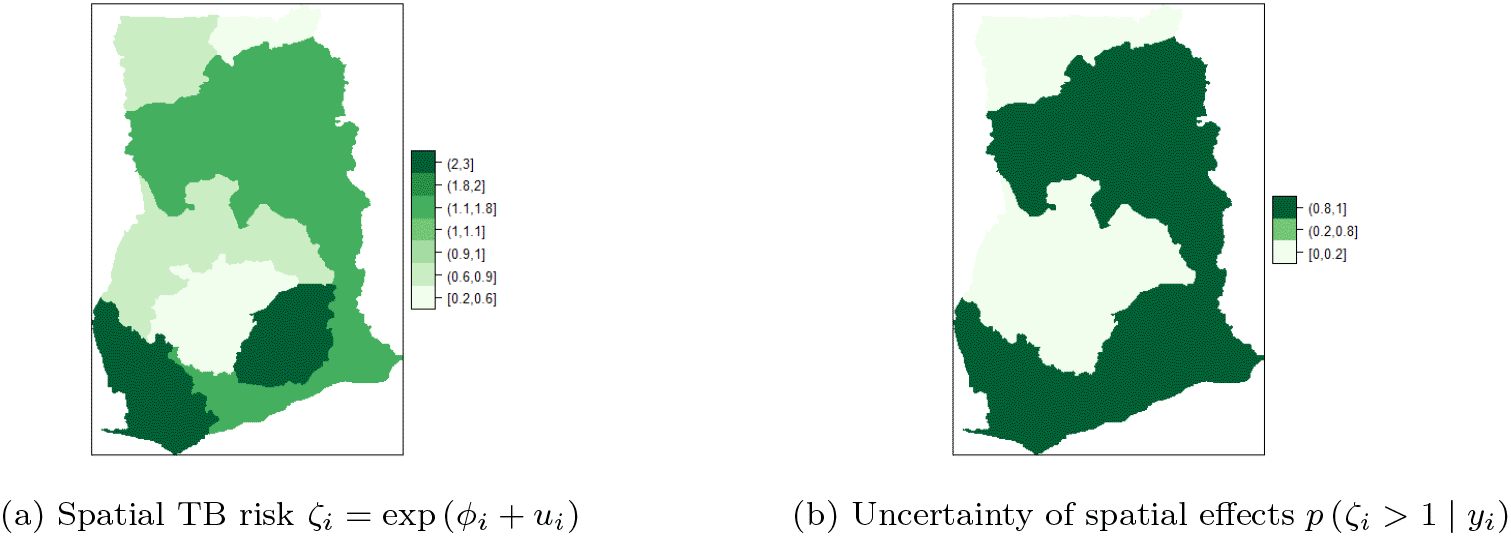
Figure 8a shows the map of spatial trend ${\zeta }_i,$ for the 10 regions and Figure 8b is the map of the posterior probabilities defined as $p\left({\zeta }_i>1|y_i\right).$ Figure 8a shows that there is high risk of TB in the Eastern and Western regions. There is high risk (i.e. in the range 1.1-1.8) and clustering among the neighboring regions; Volta, Northern, Central, and Greater Accra regions. Upper East and Ashanti regions have the lowest risk (0.2,0.6) followed by Upper West and Brong Ahafo (0.6-0.9). The results account for the high variability captured by the unstructured component and the low variability captured by the structured component of the area-specific trend. The posterior probabilities in Figure 8b indicate low risk (below 1) and relatively low level of associated uncertainty.¹⁶ The time effect is not significant and there is no significant interaction between space and time. This observation accounts for the inaccuracy of Model II (i.e. Equation (10)) and Model III (i.e. Equation (9)) for the TB data.

Figure 8. Spatial and uncertainty of TB risk, using space-time models.

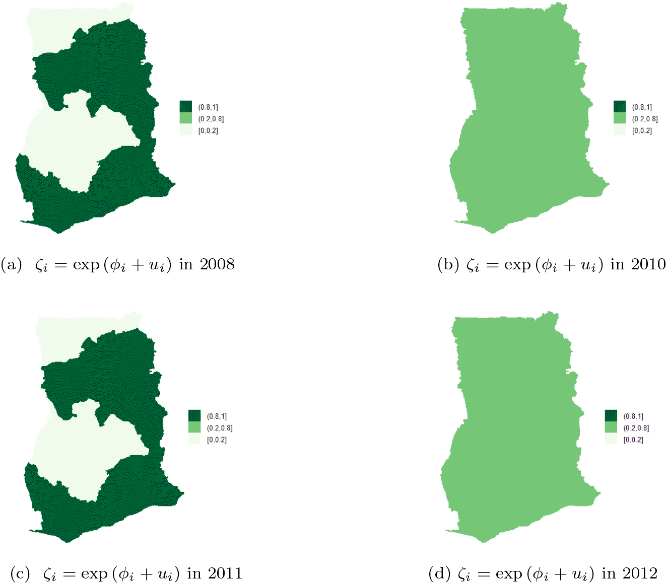
Next, the posterior probabilities of each region by year was evaluated. The results indicate that time has no significant effect on the space-time pattern of TB cases as shown in Figure 9a-d. The risk of TB infection is almost the same across the 10 regions. Figure 9a shows that there is relatively high risks (in the range 0.8-1) in the Northern, Volta, Eastern, Western, Central, and Greater Accra regions, while Upper East, Upper West, Brong Ahafo, and Ashanti regions have low relative risk (i.e. between 0-0.2). The results exhibit clear clustering of risk among neighboring regions associated with low variability or uncertainty. In the year 2010, all the regions had risks in the range 0.2-0.8, see Figure 9b. Similar observations can be made in year 2011 and the rest of the years shown in the figure. The results imply that it is sufficient to use only spatial models to estimate the risk of TB across the 10 regions of Ghana.

Figure 9. Spatial pattern of TB cases from 2008 to 2012.

Space-time models with covariate adjustments

It can be observed in Table 5, that Model I of the space-time models has the lowest DIC, mean deviance $\overline{D}$ and a high number of effective parameters $\mathit{pD}$. The indicators show that the classical parametric formulation of Ref. 23 (see Equation 7) is still the most accurate model among the three space-time models, for the TB data.

Table 6 shows negligible risk of TB across the 10 regions of Ghana. Similarly, the TB cases over time is statistically insignificant as observed previously. The precision parameter ${\tau }_u$ indicates very low variability in the risk of TB detection among the regions and much clustering of risk between neighboring regions exhibited by high precision parameter ${\tau }_{\varphi }$ values for the spatial structure. High precision characterized by ${\tau }_{\delta }$ indicates lower variability associated with ${\delta }_i.$ This further indicates that there is no significant interaction between space and time as well as global trend $\rho$ and areas-specific trend ${\delta }_i.$ Hence, the area-specific trend ${\delta }_i$ is less remarked than the mean trend.

The results in Table 6 also revealed that TB success rate significantly increases TB cases by 11%. Also, knowledge about TB significantly reduces TB cases by approximately 2%, while increasing TB cure rate, significantly reduces detection by 8%. Awareness that TB is airborne increases TB detection by approximately 25%. That is, more people are willing to participate in TB testing to know their status leading to more case detections. It was also observed that HIV prevalence and high income significantly increases TB detection by 27% and approximately 4%, respectively. Literacy significantly reduces the risk of TB detection by approximately 14%.

Figure 10a shows the spatial trend ${\zeta }_i$ for the 10 regions and Figure 10b shows the posterior probabilities defined by $p\left({\zeta }_i>1|y_i\right).$ Figure 10a shows that TB cases risk is higher and clustered in the Volta, Brong Ahafo, Ashanti, Eastern, Western and Greater Accra regions (ranging from 1-1.1) while there is low risk in the Upper East, Upper West, Northern, and Central regions. Thus, there is high and similarity/clustering of risks among neighboring regions. After covariate adjustments, there is low risk $\left(\mathrm{0.6,1}\right)$ in the Upper East, Upper West, Northern and Central regions. These observations account for the low variability captured by both the unstructured and structured components of the area-specific trend.

Figure 10. Posterior probabilities and relative risk of TB in the 10 regions of Ghana, using Model I with covariate adjustments.

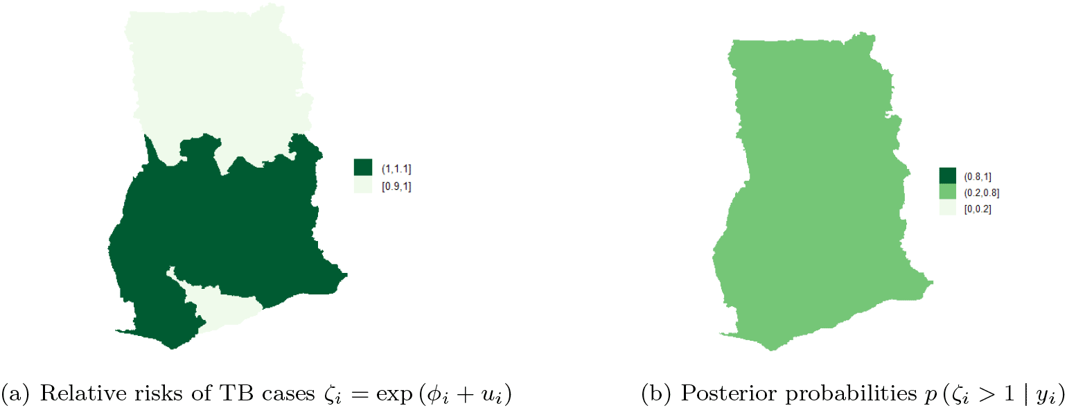
Figure 10b shows the posterior probabilities, it can be observed that all the regions have low relative risks (i.e. in the interval 0.2-0.8) after adjusting the covariates. Since the time effect is negligible, there is no interaction between space and time. This observation accounts for the inaccuracy of Model II (10) and Model III (9) for the TB data. The posterior probabilities of the region after covariate adjustments (in the period 2008-2017), showed that the risks of TB across the 10 regions are the same/clustered in the range 0.2-0.8 (this observation is the same as the one made in Figure 10b).