Using Mathematical Modeling in Environmental Sustainability to Study The Ecological Balance Between A Predator That Feeds on Two Types of Prey

Haider Ghanem Sufaeh

doi:10.12688/f1000research.172164.1

Home Browse Using Mathematical Modeling in Environmental Sustainability to Study...

ALL Metrics

-

Views

-

Downloads

Get PDF

Get XML

Export

▬

✚

Research Article

Using Mathematical Modeling in Environmental Sustainability to Study The Ecological Balance Between A Predator That Feeds on Two Types of Prey

[version 1; peer review: awaiting peer review]

Haider Ghanem Sufaeh

PUBLISHED 15 Dec 2025

Author details Author details

Department of Civil Techniques, Middle Technical University, Baghdad, Baghdad Governorate, Iraq

Haider Ghanem Sufaeh
Roles: Conceptualization, Data Curation, Formal Analysis, Funding Acquisition, Investigation, Methodology, Project Administration, Resources, Software, Supervision, Validation, Visualization, Writing – Original Draft Preparation, Writing – Review & Editing

OPEN PEER REVIEW

REVIEWER STATUS AWAITING PEER REVIEW

This article is included in the Fallujah Multidisciplinary Science and Innovation gateway.

Abstract

Background

Cooperative interactions between species play a key role in ecosystem persistence, yet most predator–prey models neglect mutualistic effects between prey species.

Methodology

We formulate a new three-dimensional ecological model describing one predator feeding on two cooperative prey populations, modeled by a system of nonlinear ordinary differential equations. We prove the positivity and boundedness of solutions, determine all biologically meaningful equilibrium points and establish their local and global stability using linearization, Lyapunov functions and the Routh–Hurwitz criteria. We then perform a bifurcation analysis with respect to key parameters, such as natural growth, natural mortality and predator attack and conversion rates. Finally, we carry out numerical simulations in MATLAB to illustrate and complement the analytical results.

Results

The analysis shows that, for a realistic set of parameter values, the system admits a unique interior equilibrium that is globally asymptotically stable, and no periodic dynamics are observed. Variations in the growth rates of both prey, the predator mortality rate and the attack and conversion rates can shift the stability of equilibria and generate transcritical bifurcations. The cooperative interaction between the two prey populations enlarges the parameter region that ensures coexistence and improves the long-term persistence of all species. Numerical simulations confirm the analytical predictions and visualize the trajectories converging to the stable equilibrium.

Conclusions

The proposed model clarifies how mutualistic interactions among prey species can stabilize predator–prey systems and enhance ecosystem sustainability. The theoretical framework and numerical results may be used as a reference for further ecological modeling that incorporates cooperation, harvesting or environmental disturbances.

Keywords

Formulation of mathematical model, Existence of equilibrium points, Local stability analysis, Globally analysis, Numerically simulation.

Corresponding author: Haider Ghanem Sufaeh

Competing interests: No competing interests were disclosed.

Grant information: The author(s) declared that no grants were involved in supporting this work.

Copyright: © 2025 Ghanem Sufaeh H. This is an open access article distributed under the terms of the Creative Commons Attribution License, which permits unrestricted use, distribution, and reproduction in any medium, provided the original work is properly cited.

How to cite: Ghanem Sufaeh H. Using Mathematical Modeling in Environmental Sustainability to Study The Ecological Balance Between A Predator That Feeds on Two Types of Prey [version 1; peer review: awaiting peer review]. F1000Research 2025, 14:1397 (https://doi.org/10.12688/f1000research.172164.1) First published: 15 Dec 2025, 14:1397 (https://doi.org/10.12688/f1000research.172164.1) Latest published: 15 Dec 2025, 14:1397 (https://doi.org/10.12688/f1000research.172164.1)

Introduction

Environmental sustainability is an important concept that aims to preserve the Earth’s natural and environmental resources to ensure the quality of life today and in the future, as it depends on achieving a balance between human needs, preserving the environment, and eliminating negative impacts on the ecosystem. Diverse activities and tasks across disciplines can be represented in a mathematical model that encompasses the diversity of studies across disciplines in the environmental sustainability system. This principle (sustainability) has become widespread and can be applied to all aspects of life on Earth, at different times, and in different places, such as forests, green areas, or wetlands. Healthy forests are among the most important examples of healthy and vital systems for sustainability.^1–3 To provide healthy and vital forests to ensure environmental sustainability, the balance in the ecosystem must be studied through a mathematical model that examines organisms and their relationship with each other, especially the relationship of coexistence between living organisms, as well as reducing the severity of predation by predators on organisms that are considered easy prey. This was the basis of our study. Many researchers in the field of ecosystems and the study of cases of environmental stability and equilibrium have expressed the system using a mathematical model that studies the relationship between living organisms. These systems have become widespread in all sciences and disciplines, and include diverse sciences in the biological sciences, infectious diseases, physiology, environmental sciences, immunology, economics, chemical reactions, genetics, and pharmacodynamics.^4,5 In addition to these systems, there are universally agreed upon principles that the relationship between living organisms (humans, animals, and plants) constitutes a key link in the chain of universal life. This relationship is represented by an interaction represented by a mathematical model, which is an important application of applied mathematics in the animal world; weak animals (prey) can become a major food source for other animals (predators). In this case, the role of mathematicians is to choose the model that achieves the principles of safety and environmental sustainability.^6,7 This interaction is called a predator-prey relationship.^8–11 Two different types of animals and organisms can also interact in a mutually beneficial relationship, known as symbiosis.¹² An example is the nectar of flowering plants and bees that feed on it. Nectar is the food of bees, whereas bees pollinate flowers.^13,14 The other interaction, which is one of the most important, can be represented by a single food source shared between two or more species of organisms competing for it or organisms competing for survival.¹⁵ This type can be described by a set of mostly nonlinear equations (perhaps algebraic or differential equations). Therefore, the science of dynamic behavior in biological systems has become dominant in modeling science over the last few years. One of the important issues that must be highlighted when studying the predator-prey model is that logistic growth reaches the highest carrying capacity in the prey community if the predator is absent, and gives complete equilibrium and an ascending growth curve for the prey in the absence of predators. For this reason, most modelers and biologists have devoted their attention and time to this species, studying it closely and among them.^16–21 Hence, biologists have begun to use these models to help them understand and study the biological aspects of organisms under their natural conditions.^22–25 Recently, many researchers have been interested in a specific issue, which is the fear of the prey and the effect of its fear of the predator, and discovered through mathematical results that this effect is very negative.^26,27 In addition, a study was conducted in^28,29 on the impact of direct killing and hunting on birds and invertebrates during their breeding seasons to clarify how predators are affected. A predator-prey model with non-local competition can produce complex dynamics, such as spatiotemporal patterns and spatially heterogeneous periodic solutions. See³⁰ Ghanem, H. and Majeed studied the dynamics of a predator-prey model including two types of epidemics with harvest. The basic structure of a mathematical model with a biological meaning and character that can be studied accurately and carefully, based on the most important members of the population, is the prey and predator, which is described as the density of the prey consumed per unit of time by the predators.^31–33 Latest I have come up with Ghanem, H. and Khaleefah, K in,³⁴ a special study on the prey and predator patterns of Lake Victoria tilapia, snook, and coptodon, and recommendations for their conservation from overfishing. The study in this research is based on proposing a mathematical environmental (biological) model for living organisms, achieving a large part of the principles of environmental sustainability by creating the necessary conditions for coexistence and exchange of benefits between organisms that were considered prey for the purpose of controlling their extinction, which causes the death of a large part of the environment and an effective resource in the environmental balance, which consists of a system of differential equations. The local and global stability were analyzed and discussed, and the results were analyzed using numerical simulations related to the conditions of equilibrium and environmental sustainability. The results were positive for the purpose of providing a sustainable ecosystem.

Formulation of mathematical model

Consider the proposed cooperative ecological mathematical model of three organisms, which involves a predator feeding on two prey species in a symbiotic relationship and exchanging food and resources for survival. Lotka-Volterra considered the response function (Holling function of the first kind) as a response dynamic process. Therefore, the population density hypothesis represented by the symbols X(T), Y(T), and Z(T) is that the first, second, and predator feed on them at any time (T) respectively. The growth density of the two prey groups represented a positive natural growth rate for both species (logistic growth). The relationship between organisms was described according to their effect on each other, where coexistence was considered a close relationship between the first and second prey, and the third organism was considered a predator of the first two species, in addition to the intense competition within each community, which may have been for food or for females during the mating season. Therefore, we describe how population density changes over time for the proposed species by partitioning the system into a set of three independent ordinary differential equations. Based on this model, see the following system:

(1)

\begin{matrix} \frac{dX}{dT} = a_{1} (1 - X) X + bXY - λ_{1} XZ - d_{1} X \\ \frac{dY}{dT} = a_{2} (1 - Y) Y + cXY - λ_{2} YZ - d_{2} Y \\ \frac{dZ}{dT} = e_{1} λ_{1} XZ + e_{2} λ_{2} YZ - (d_{3} + d_{4} Z) Z \end{matrix}

With initial values of variables (X(0) ⩾ 0, Y(0) ⩾ 0, Z(0) ⩾ 0) $.$

The Table 1 describes the basic parameters of the model (1).

Table 1. The parameters of the model (1).

Parameters	Description of parameters
$a_{i}, i = 1, 2$	Natural growth rate of the first prey X and the second prey Y respectively.
$b,$ $c$	The commensal relationship between the first prey X and the second prey Y.
$λ_{i}, i = 1, 2$	Maximum predation rates from first prey X and second prey Y to predator Z respectively.
$d_{i}, i = 1, 2, 3, 4$	The natural rate of death for the three organisms, which are the first prey, the second prey, their predator and the competition within the predator community respectively.
$e_{i}, i = 1, 2$	Food conversion ratios from the two organisms to predator.

We study the initial conditions of model (1) in space $(R_{+}^{3})$ and show that the functions of model (1) are continuous and differentiable on $(R_{+}^{3})$ , thus, the Lipschitz condition is satisfied, which is proof of the existence and uniqueness of model (1). In addition, all solutions of model (1) with its nonnegative initial condition are completely determined, as shown in the following theorem:

Theorem 1:

The solutions to Model (1) are uniformly bounded.

Proof:

Let $x (t), y (t), z (t)$ be any solution to model (1), and define the function.

$W (t) = x (t) + y (t) + z (t),$ We differentiate the function with respect to time and then the time derivative of $W (t)$ over all of the form (1) yields:

\frac{dW}{dt} \leq a_{1} x + a_{2} y + (c + b) xy + e_{1} λ_{1} xz + e_{2} λ_{2} yz - uW = V - uW .

Where $u = min {d_{1}, d_{2}, d_{3}}$ and $V = a_{1} x + a_{2} y + (c + b) xy + e_{1} λ_{1} xz + e_{2} λ_{2} yz .$

Now, based on the Gronwell theory, gets that:

0 < W (t) \leq W (0) e^{- ut} + \frac{V}{u} (1 - e^{- ut})

This gives: $lim_{t \to \infty} W (t) \leq$ $\frac{V}{u} .$ Therefore, the proof is complete, because it is independent of the initial conditions.

Existence of equilibrium points

The study in this part is concerned with searching for the existence of possible and expected (fixed) equilibrium points for Model (1), where it was noted that no more than seven points are the possible equilibrium points.

1- The point that always exists is the simple equilibrium point, $E_{0}$ = (0, 0, 0).
2- The point called the equilibrium point of the axial ${\hat{E}}_{1}$ = ( $\hat{x}$ , 0, 0) where $\hat{x} = \frac{a_{1} - d_{1}}{a_{1}}$ exists if the following condition is met:

(2)

(a_{1} > d_{1})

3- The third equilibrium point ${\bar{E}}_{2}$ = ( $0$ , $\bar{y}$ , 0) where $\bar{y} = \frac{a_{2} - d_{2}}{a_{2}}$ exists under the following conditions:

(3)

(a_{2} > d_{2})

4- The fourth point of equilibrium is called the predation-free point ${\tilde{E}}_{3}$ = ( $\tilde{x}$ , $\tilde{y}$ , 0) where

\tilde{x} = \frac{b (a_{2} - d_{2}) + c (a_{1} - d_{1})}{(c b - a_{1} a_{2})} and \tilde{y} = \frac{a_{1} (\tilde{x} - 1) + d_{2}}{b}

This point is present if we adopt conditions $(2)$ and $(3)$ in addition to the following condition:

(4)

(\tilde{x} > 1) and (c b > a_{1} a_{2})

5- The fifth point of balance ${\dot{E}}_{4} = (0$ , $\dot{y}, \dot{z}$ ) where $\dot{y} = \frac{a_{2} d_{4} - d_{2} d_{4} + λ_{2} d_{3}}{a_{2} d_{4} + e_{2} {(λ_{2})}^{2}}$ and $\dot{z} = \frac{e_{2} λ_{2} \dot{y} - d_{3}}{d_{4}}$

${\dot{E}}_{4}$ is found based on condition (3) add the following condition:

(5)

(e_{2} λ_{2} \dot{y} > d_{3})

6- Sixth balance point ${\overset{̿}{E}}_{5} = (\overset{̿}{x}, 0, \overset{̿}{z})$ where:

\overset{̿}{x} = \frac{a_{1} d_{4} - d_{1} d_{4} + λ_{1} d_{3}}{a_{1} d_{4} + e_{1} {(λ_{1})}^{2}} and \overset{̿}{z} = \frac{e_{1} λ_{1} \overset{̿}{x} - d_{3}}{d_{4}}

${\overset{̿}{E}}_{5}$ is found based on condition (2) add the following condition:

(6)

(e_{1} λ_{1} \overset{̿}{x} > d_{3})

7- The seventh point is called the positive balance point or the coexistence point ${E_{6}}^{*} = (x^{*}, y^{*}, z^{*})$

Where:

\begin{matrix} x^{*} = \frac{(a_{1} - d_{1} - λ_{2} z^{*}) (c b - a_{1} a_{2}) - a_{1} b (λ_{2} z^{*} + d_{2}) + a_{1} b (a_{2} + c) - cb (λ_{1} z^{*} + d_{1})}{(c b - a_{1} a_{2})} \\ y^{*} = \frac{a_{1} a_{2} + a_{1} c - c λ_{1} z^{*} - a_{1} λ_{2} z^{*} - c d_{1} - a_{1} d_{2}}{(c b - a_{1} a_{2})} \\ z^{*} = \frac{{S_{1}}^{*}}{{S_{2}}^{*} + {S_{3}}^{*}} \end{matrix}

\begin{matrix} {S_{1}}^{*} = - (c e_{2} λ_{1} λ_{2} + a_{1} e_{2} {(λ_{2})}^{2} - (c b - a_{1} a_{2}) (e_{1} λ_{1} λ_{2} - d_{4}) + c b e_{2} {(λ_{1})}^{2} + b a_{1} e_{1} λ_{1} λ_{2}) \\ {S_{2}}^{*} = a_{1} a_{2} e_{2} λ_{2} + c a_{1} e_{2} λ_{2} - c e_{2} λ_{2} d_{1} - a_{1} e_{2} λ_{2} d_{2} + (cb - a_{1} a_{2}) (e_{1} λ_{1} d_{1} - d_{3}) \\ {S_{3}}^{*} = a_{1} a_{2} e_{1} λ_{1} b + c a_{1} e_{1} λ_{1} b - a_{1} e_{1} λ_{1} b d_{2} \end{matrix}

${E_{6}}^{*}$ is found based on conditions (2), (3) and (4) add the following condition:

Where

(7)

\frac{d_{4}}{λ_{2}} < e_{1} λ_{1} < \frac{d_{3}}{(a_{1} - d_{1})}

(8)

\begin{matrix} (c b - a_{1} a_{2}) + (a_{1} e_{1} λ_{1} - e_{1} λ_{1} d_{1} - d_{3}) - a_{1} e_{1} λ_{1} b d_{2} > {S_{4}}^{*} \\ {S_{4}}^{*} = (a_{1} a_{2} - a_{1} d_{2}) e_{2} λ_{2} + (a_{1} c - d_{1} c) e_{2} λ_{2} + (a_{1} a_{2} + a_{1} c) e_{1} λ_{1} . \end{matrix}

Local stability analysis

The stability analysis of model (1) is dealt with in this section for all stability points, and by calculating the Jacobian matrix $J (X, Y, Z)$ and studying all cases of convergence and stability depending on the resulting eigenvalues to compensate for the points of model (1) that were obtained, where the matrix can be written as follows:

J (X, Y, Z) = [\begin{matrix} a_{1} - 2 a_{1} x + by - λ_{1} z - d_{1} & bx & - λ_{1} x \\ c y & a_{2} - 2 a_{2} y + c x - λ_{2} z - d_{2} & - λ_{2} y \\ e_{1} λ_{1} z & e_{2} λ_{2} z & e_{1} λ_{1} x + e_{2} λ_{2} y - d_{3} - 2 d_{4} z \end{matrix}]

System (1) contains a distinct equation for matrix close to $E_{0}$ in the following form:

J (E_{0}) = [\begin{matrix} (a_{1} - d_{1}) & 0 & 0 \\ 0 & (a_{2} - d_{2}) & 0 \\ 0 & 0 & - d_{3} \end{matrix}]

Given by:

(9)

(Г_{1} - (a_{1} - d_{1})) (Г_{2} - (a_{2} - d_{2})) (Г_{3} + d_{3}) = 0

Consider Equation (9) based on condition (2) we get $(Г_{1} > 0) and$ by (3) we have that $(Г_{2} > 0)$ and $(Г_{3} = - d_{3} < 0)$ $so, E_{0}$ unstable point.

The Jacobian matrix for equilibrium point ${\hat{E}}_{1}$ in model (1) is written as follows:

J ({\hat{E}}_{1}) = [\begin{matrix} - a_{1} \hat{x} & b \hat{x} & - λ_{1} \hat{x} \\ 0 & a_{2} + c \hat{x} - d_{2} & 0 \\ 0 & 0 & e_{1} \hat{x} λ_{1} - d_{3} \end{matrix}]

The following equation is the characteristic equation of $J ({\hat{E}}_{1})$ and is defined as follows:

(10)

(- a_{1} \hat{x} - {\hat{Г}}_{1}) (a_{2} + c \hat{x} - d_{2} - {\hat{Г}}_{2}) (e_{1} \hat{x} λ_{1} - d_{3} - {\hat{Г}}_{3}) = 0

Where ${\hat{Г}}_{1} = - a_{1} \hat{x}$ , ${\hat{Г}}_{2} = a_{2} + c \hat{x} - d_{2}$ , ${\hat{Г}}_{3} = e_{1} \hat{x} λ_{1} - d_{3}$

Consider Equation (10) based on condition (3) we get $({\hat{Г}}_{2} > 0)$ and $({\hat{Г}}_{1} = - a_{1} \hat{x} < 0)$

Without the need for an eigenvalue indication ${\hat{Г}}_{3}$ , $so, {\hat{E}}_{1}$ (Saddle) unstable point.

The Jacobian matrix for equilibrium point ${\bar{E}}_{2}$ in model (1) is written as follows:

J ({\bar{E}}_{2}) = [\begin{matrix} a_{1} - d_{1} + b \bar{y} & 0 & 0 \\ c \bar{y} & - a_{2} \bar{y} & - λ_{2} \bar{y} \\ 0 & 0 & e_{2} λ_{2} \bar{y} - d_{3} \end{matrix}]

The following equation is the characteristic equation of $J ({\bar{E}}_{2})$ and is defined as follows:

(11)

(a_{1} - d_{1} + b \bar{y} - {\bar{Г}}_{1}) (- a_{2} \bar{y} - {\bar{Г}}_{2}) (e_{2} \bar{y} λ_{2} - d_{3} - {\bar{Г}}_{3}) = 0

Consider Equation (11) based on condition (2) we get $({\bar{Г}}_{1} > 0)$ and $({\bar{Г}}_{2} = - a_{2} \bar{y} < 0)$ $so, {\bar{E}}_{2}$ (Saddle) unstable point.

The Jacobian matrix for equilibrium point ${\tilde{E}}_{3}$ in model (1) is written as follows:

J ({\tilde{E}}_{3}) = [\begin{matrix} a_{1} - 2 a_{1} \tilde{x} + b \tilde{y} - d_{1} & b \tilde{x} & - λ_{1} \tilde{x} \\ c \tilde{y} & a_{2} - 2 a_{2} \tilde{y} + c \tilde{x} - d_{2} & - λ_{2} \tilde{y} \\ 0 & 0 & e_{1} λ_{1} \tilde{x} + e_{2} λ_{2} \tilde{y} - d_{3} \end{matrix}]

The following equation is the characteristic equation of $J ({\tilde{E}}_{3})$ and is defined as follows:

(12)

{(\tilde{Г})}^{3} + {\tilde{A}}_{1} {(\tilde{Г})}^{2} + {\tilde{A}}_{2} (\tilde{Г}) + {\tilde{A}}_{3} = 0

where

{\tilde{A}}_{1} = d_{3} - e_{1} λ_{1} \tilde{x} - e_{2} λ_{2} \tilde{y} + a_{1} \tilde{x} + a_{2} \tilde{y} .

{\tilde{A}}_{2} = a_{2} d_{3} \tilde{y} + a_{2} e_{1} λ_{1} \tilde{x} \tilde{y} + a_{2} e_{2} λ_{2} {(\tilde{y})}^{2} + a_{1} \tilde{x} d_{3} + a_{1} e_{1} λ_{1} {(\tilde{x})}^{2} - a_{1} e_{2} λ_{2} \tilde{x} \tilde{y} + a_{1} a_{2} \tilde{x} \tilde{y} + cb \tilde{x} \tilde{y} .

{\tilde{A}}_{3} = a_{1} a_{2} \tilde{x} \tilde{y} d_{3} - e_{1} a_{1} a_{2} \tilde{x} \tilde{y} - a_{1} a_{2} e_{2} λ_{2} \tilde{x} {(\tilde{y})}^{2} + bc e_{1} λ_{1} \tilde{y} {(\tilde{x})}^{2} + bc e_{2} λ_{2} \tilde{x} {(\tilde{y})}^{2} + bc \tilde{x} \tilde{y} d_{3} .

According to the Routh-Hurwitz criterion, there are roots with a negative real part of Equation (12) if and only if ${\tilde{A}}_{1} > 0, {\tilde{A}}_{3} > 0 and \tilde{∆} = {\tilde{A}}_{1} {\tilde{A}}_{2} - {\tilde{A}}_{3} > 0 .$

$({\tilde{A}}_{1} > 0$ and ${\tilde{A}}_{3} > 0)$ based on the condition (4) add the following conditions:

(13)

\begin{matrix} a_{1} > e_{1} λ_{1} \\ a_{2} > e_{2} λ_{2} \end{matrix}}

(14)

e_{1} λ_{1} \tilde{x} > d_{3} > e_{1} λ_{1}

$Now, \tilde{∆} = {\tilde{A}}_{1} {\tilde{A}}_{2} - {\tilde{A}}_{3} .$

We have that $({\tilde{A}}_{1} > 0$ and ${\tilde{A}}_{3} > 0)$ with the above conditions.

And accordingly, $\tilde{∆} = {\tilde{A}}_{1} {\tilde{A}}_{2} - {\tilde{A}}_{3} > 0 . If the condition is met {\tilde{A}}_{1} {\tilde{A}}_{2} > {\tilde{A}}_{3} .$

So, ${\tilde{E}}_{3}$ it is locally asymptotical stable, otherwise unstable.

The Jacobian matrix for equilibrium point ${\dot{E}}_{4}$ in model (1) is written as follows:

J ({\dot{E}}_{4}) = [\begin{matrix} \dot{M} & 0 & 0 \\ c \dot{y} & - a_{2} \dot{y} & - λ_{2} \dot{y} \\ e_{1} λ_{1} \dot{z} & e_{2} λ_{2} \dot{z} & - d_{4} \dot{z} \end{matrix}],

where

\dot{M} = a_{1} + b \dot{y} - λ_{1} \dot{z} - d_{1} .

The following equation is the characteristic equation of $J ({\dot{E}}_{4})$ and is defined as follows:

(15)

{(\dot{Г})}^{3} + {\dot{R}}_{1} {(\dot{Г})}^{2} + {\dot{R}}_{2} (\dot{Г}) + {\dot{R}}_{3} = 0

Where ${\dot{R}}_{1} = a_{2} \dot{y} + d_{4} \dot{z} - \dot{M}$ , ${\dot{R}}_{2} = e_{2}$ ${(λ_{2})}^{2} \dot{z} \dot{y} + a_{2} \dot{y} d_{4} \dot{z -} (a_{2} \dot{y} + d_{4} \dot{z}) \dot{M}$ , ${\dot{R}}_{3} = e_{2}$ ${(λ_{2})}^{2} \dot{z} \dot{y} \dot{M} - a_{2} \dot{y} d_{4} \dot{z} \dot{M} .$

According to the Routh-Hurwitz criterion, there are roots with a negative real part of Equation (15) if and only if ${\dot{R}}_{1} > 0, {\dot{R}}_{3} > 0 and \dot{∆}$ $= {\dot{R}}_{1} {\dot{R}}_{2} - {\dot{R}}_{3} > 0 .$

$({\dot{R}}_{1} > 0$ and ${\dot{R}}_{3} > 0)$ if the following conditions hold:

(16)

a_{1} + b \dot{y} < λ_{1} \dot{z} + d_{1}

(17)

a_{2} d_{4} > e_{2} {(λ_{2})}^{2}

$Now,$ $\dot{∆}$ $= {\dot{R}}_{1} {\dot{R}}_{2} - {\dot{R}}_{3}$

We have that ${\dot{R}}_{1} > 0$ and ${\dot{R}}_{3} > 0$ with the above conditions.

And accordingly, $\dot{∆}$ $= {\dot{R}}_{1} {\dot{R}}_{2} - {\dot{R}}_{3} > 0 . If the condition is met ({\dot{R}}_{1} {\dot{R}}_{2} > {\dot{R}}_{3}) .$

So, ${\dot{E}}_{4}$ it is locally asymptotical stable, otherwise unstable.

The Jacobian matrix for equilibrium point ${\overset{̿}{E}}_{5}$ in model (1) is written as follows:

J ({\overset{̿}{E}}_{5}) = [\begin{matrix} - a_{1} \overset{̿}{x} & b \overset{̿}{x} & - λ_{1} \overset{̿}{x} \\ 0 & \overset{̿}{W} & 0 \\ e_{1} λ_{1} \overset{̿}{z} & e_{2} λ_{2} \overset{̿}{z} & - d_{4} \overset{̿}{z} \end{matrix}],

where

\overset{̿}{W} = a_{2} + c \overset{̿}{x} - λ_{2} \overset{̿}{z} - d_{2} .

The following equation is the characteristic equation of $J ({\overset{̿}{E}}_{5})$ and is defined as follows:

(18)

{(\overset{̿}{Г})}^{3} + {\overset{̿}{K}}_{1} {(\overset{̿}{Г})}^{2} + {\overset{̿}{K}}_{2} (\overset{̿}{Г}) + {\overset{̿}{K}}_{3} = 0

Where ${\overset{̿}{K}}_{1} = d_{4} \overset{̿}{z} + a_{1} \overset{̿}{x} - \overset{̿}{W}$ , ${\overset{̿}{K}}_{2} = a_{1} d_{4} \overset{̿}{z} \overset{̿}{x} - \overset{̿}{W} d_{4} \overset{̿}{z} - a_{1} \overset{̿}{x} \overset{̿}{W} - e_{1} \overset{̿}{z} \overset{̿}{x} {(λ_{1})}^{2}$ , ${\overset{̿}{K}}_{3} =$ $e_{1} \overset{̿}{z} \overset{̿}{x} {(λ_{1})}^{2} \overset{̿}{W} - a_{1} d_{4} \overset{̿}{z} \overset{̿}{x} \overset{̿}{W} .$

According to the Routh-Hurwitz criterion, there are roots with a negative real part of Equation (18) if and only if

{\overset{̿}{K}}_{1} > 0, {\overset{̿}{K}}_{3} > 0 and \overset{̿}{∆} = {\overset{̿}{K}}_{1} {\overset{̿}{K}}_{2} - {\overset{̿}{K}}_{3} > 0 .

$({\overset{̿}{K}}_{1} > 0$ and ${\overset{̿}{K}}_{3} > 0)$ if the following conditions hold:

(19)

a_{2} + c \overset{̿}{x} < d_{2} + λ_{2} \overset{̿}{z}

(20)

e_{1} {(λ_{1})}^{2} < a_{1} d_{4}

Now, $\overset{̿}{∆} = {\overset{̿}{K}}_{1} {\overset{̿}{K}}_{2} - {\overset{̿}{K}}_{3}$

We have that $({\overset{̿}{K}}_{1} > 0$ and ${\overset{̿}{K}}_{3} > 0)$ with the above conditions.

And accordingly, $\overset{̿}{∆} = {\overset{̿}{K}}_{1} {\overset{̿}{K}}_{2} - {\overset{̿}{K}}_{3} > 0 If the condition is met ({\overset{̿}{K}}_{1} {\overset{̿}{K}}_{2} > {\overset{̿}{K}}_{3}) .$

So, ${\overset{̿}{E}}_{5}$ it is locally asymptotical stable, otherwise unstable.

The Jacobian matrix for equilibrium point ${E_{6}}^{*}$ in Model (1) is expressed as follows:

J ({E_{6}}^{*}) = [\begin{matrix} - a_{1} x^{*} & b x^{*} & - λ_{1} x^{*} \\ c y^{*} & - a_{2} y^{*} & - λ_{2} y^{*} \\ e_{1} λ_{1} z^{*} & e_{2} λ_{2} z^{*} & - d_{4} z^{*} \end{matrix}] .

The following equation is the characteristic equation of $J ({E_{6}}^{*})$ and is defined as follows:

(21)

{(Г^{*})}^{3} + {V^{*}}_{1} {(Г^{*})}^{2} + {V^{*}}_{2} (Г^{*}) + {V^{*}}_{3} = 0

Where ${V^{*}}_{1} = a_{1} x^{*} + a_{2} y^{*} + d_{4} z^{*}$ , ${V^{*}}_{2} = a_{1} d_{4} z^{*} x^{*} + a_{2} d_{4} z^{*} y^{*} - e_{2} z^{*} y^{*} {(λ_{2})}^{2} + a_{1} a_{2} y^{*} x^{*} + b c y^{*} x^{*} - e_{1} z^{*} x^{*} {(λ_{1})}^{2}$ , ${V^{*}}_{3} = (b e_{1} - c e_{2}) λ_{1} λ_{2} z^{*} x^{*} y^{*} + (a_{2} d_{4} - e_{2} λ_{2}) a_{1} z^{*} x^{*} y^{*} + (b c d_{4} - a_{2} e_{1} {(λ_{1})}^{2}) z^{*} x^{*} y^{*}$ .

According to the Routh-Hurwitz criterion, there are roots with a negative real part of Equation (21) if and only if

{V^{*}}_{1} > 0, {V^{*}}_{3} > 0 and ∆^{*} = {V^{*}}_{1} {V^{*}}_{2} - {V^{*}}_{3} > 0 .

$({V^{*}}_{1} > 0$ and ${V^{*}}_{3} > 0)$ based on the condition (17) add the following conditions:

(22)

b e_{1} > c e_{2}

(23)

b c d_{4} > a_{2} e_{1} {(λ_{1})}^{2}

Now, $∆^{*} = {V^{*}}_{1} {V^{*}}_{2} - {V^{*}}_{3} .$

We have that $({V^{*}}_{1} > 0$ and ${V^{*}}_{3} > 0)$ with the above conditions.

And accordingly, $∆^{*} = {V^{*}}_{1} {V^{*}}_{2} - {V^{*}}_{3} > 0 . If the condition is met ({V^{*}}_{1} {V^{*}}_{2} > {V^{*}}_{3}) .$

So, $({E_{6}}^{*})$ it is locally asymptotical stable, otherwise unstable.

Globally analysis

The comprehensive study and analysis in particular is studied in this section for the balanced points found in the previous section, called the local stability of model (1), and that is by using the Lyapunov function that satisfies the conditions of global equilibrium, as shown in the following theorems:

Lemma:

(Lyapunov stability theorem):

Suppose that $x^{*}$ be an equilibrium point of system (1.12) and $V : N \to R$ be an C¹ real-valued function defined on some neighborhood $N$ of $x^{*}$ with $(N \subseteq R^{n})$ such that

⋄ $V (x^{*}) = 0$ and $V (x) > 0$ for all $x \neq x^{*}$ and $x \in N$ (i.e., mean V is a positive definite function).
⋄ If $\frac{d V (x)}{dt} \leq 0$ in $N - {x^{*}}$ , then $x^{*}$ is stable.
⋄ If $\frac{d V (x)}{dt} < 0$ in $N - {x^{*}}$ , then $x^{*}$ is asymptotically stable.

Note that the function $V$ given above is known as the Lyapunov function (weak Lyapunov function) if and only if the first and second conditions hold, whereas it is known as a strict Lyapunov function (strong Lyapunov function) if and only if the first and third conditions hold. In addition, if $N$ can be chosen to be all of $R^{n}$ , then $x^{*}$ is said to be globally asymptotically stable if the first and third conditions hold.

Theorem 2:

Assume that ${\tilde{E}}_{3}$ = ( $\tilde{x}$ , $\tilde{y}$ , 0) is locally asymptotically stable. Then, point ${\tilde{E}}_{3}$ is globally asymptotically stable in space $R_{+}^{3}$ under the following conditions:

(24)

(b + c) < 2 \sqrt{a_{1} a_{2}}

(25)

- {\tilde{ω}}_{1} < {\tilde{ω}}_{2}

where

{\tilde{ω}}_{1} = (λ_{1} \tilde{x} + λ_{2} \tilde{y}) z

,

{\tilde{ω}}_{2} = - {(\sqrt{a_{1}} (x - \tilde{x}) - \sqrt{a_{1}} (y - \tilde{y}))}^{2} .

Proof:

Consider the function below:

{\tilde{G}}_{1} (x, y, z) = (c_{1} x - c_{1} \tilde{x} - c_{1} \tilde{x} ln \frac{x}{\tilde{x}}) + (c_{2} y - c_{2} \tilde{y} - c_{2} \tilde{y} ln \frac{y}{\tilde{y}}) + c_{3} z .

Choose $(c_{1} = c_{2} = c_{3} = 1)$

We differentiate the function $({\tilde{G}}_{1})$ directly with respect to time t and get:

\frac{d {\tilde{G}}_{1}}{dt} = - a_{1} {(x - \tilde{x})}^{2} + (b + c) {(x - \tilde{x})}^{2} {(y - \tilde{y})}^{2} - a_{2} {(y - \tilde{y})}^{2} - (1 - e_{1}) λ_{1} x z - (1 - e_{2}) λ_{2} y z + λ_{1} \tilde{x} z + λ_{2} \tilde{y} z - (d_{3} + d_{4} z) z .

Depending on the biological environmental facts, which are ( $e_{1} < 1$ ) and ( $e_{2} < 1)$ with condition $(24)$ we obtain the following:

\frac{d {\tilde{G}}_{1}}{dt} < - {(\sqrt{a_{1}} (x - \tilde{x}) - \sqrt{a_{1}} (y - \tilde{y}))}^{2} - (d_{3} + d_{4} z) z + (λ_{1} \tilde{x} + λ_{2} \tilde{y}) z = {\tilde{ω}}_{2} + {\tilde{ω}}_{1} .

Under condition $(25),$ $(\frac{d {\tilde{G}}_{1}}{dt}$ $< 0)$ is accepted, and it turns out that $\frac{d {\tilde{G}}_{1}}{dt}$ is definitely negative depending on the local condition; thus, $({\tilde{G}}_{1})$ is a Lyapunov function with respect to ${\tilde{E}}_{3}$ , and ${\tilde{E}}_{3}$ is close to global asymptotical stability.

Theorem 3:

Assume that ${\dot{E}}_{4} = (0$ , $\dot{y}, \dot{z}$ ) is locally asymptotically stable. Then, point ${\dot{E}}_{4}$ is Globally asymptotically stable in space $R_{+}^{3}$ under the following conditions:

(26)

λ_{2} < 2 \sqrt{a_{2} d_{4}}

(27)

{\dot{ω}}_{1} < - {\dot{ω}}_{2}

where

{\dot{ω}}_{1} = a_{1} x + c x y + b x y .

{\dot{ω}}_{2} = - {(\sqrt{a_{2}} (y - \dot{y}) - \sqrt{d_{4}} (z - \dot{z}))}^{2} - (c \dot{y} + d_{1} + a_{1} x + e_{1} λ_{1} \dot{z}) x .

Proof:

Consider the function below:

{\dot{G}}_{2} (x, y, z) = c_{1} x + (c_{2} y - c_{2} \dot{y} - c_{2} \dot{y} ln \frac{y}{\dot{y}}) + (c_{3} z - c_{3} \dot{z} - c_{3} \dot{z} ln \frac{z}{\dot{z}}) .

Choose $(c_{1} = c_{2} = c_{3} = 1)$

We differentiate the function $({\dot{G}}_{2})$ directly with respect to time t and get:

\frac{d {\dot{G}}_{2}}{dt} = a_{1} x - a_{1} {(x)}^{2} + (b + c) x y - c x \dot{y} - d_{1} x - (1 - e_{1}) λ_{1} x z - (a_{2} {(y - \dot{y})}^{2} - λ_{2} (1 - e_{2}) (y - \dot{y}) (z - \dot{z}) + d_{4} {(z - \dot{z})}^{2}) .

Depending on the biological environmental facts, which are ( $e_{1} < 1$ ) and ( $e_{2} < 1)$ with condition $(26)$ we obtain the following:

\frac{d {\dot{G}}_{2}}{dt} < a_{1} x + c x y + b x y - {(\sqrt{a_{2}} (y - \dot{y}) - \sqrt{d_{4}} (z - \dot{z}))}^{2} - (c \dot{y} + d_{1} + a_{1} x + e_{1} λ_{1} \dot{z}) x = {\dot{ω}}_{1} + {\dot{ω}}_{2} .

Under condition $(27),$ $(\frac{d {\dot{G}}_{2}}{dt}$ $< 0)$ is accepted, and it turns out that $\frac{d {\dot{G}}_{2}}{dt}$ is definitely negative, depending on the local condition; thus, $({\dot{G}}_{2})$ is a Lyapunov function with respect to ${\dot{E}}_{4}$ , and ${\dot{E}}_{4}$ is close to global asymptotical stability.

Theorem 4:

Assume that ${\overset{̿}{E}}_{5} = (\overset{̿}{x}, 0, \overset{̿}{z})$ is locally asymptotically stable. Then, point ${\overset{̿}{E}}_{5}$ is globally asymptotically stable in space $R_{+}^{3}$ under the following conditions:

(28)

λ_{1} < 2 \sqrt{a_{1} d_{4}}

(29)

{\overset{̿}{ω}}_{1} < - {\overset{̿}{ω}}_{2}

where

{\overset{̿}{ω}}_{1} = a_{2} y + c x y + b x y .

{\overset{̿}{ω}}_{2} = - {(\sqrt{a_{1}} (x - \overset{̿}{x}) - \sqrt{d_{4}} (z - \overset{̿}{z}))}^{2} - b \overset{̿}{x} y - a_{2} {(y)}^{2} - d_{2} y - e_{2} λ_{2} y \overset{̿}{z} .

Proof:

Consider the function below:

{\overset{̿}{G}}_{3} (x, y, z) = (c_{1} x - c_{1} \overset{̿}{x} - c_{1} \overset{̿}{x} ln \frac{x}{\overset{̿}{x}}) + c_{2} y + (c_{3} z - c_{3} \overset{̿}{z} - c_{3} \overset{̿}{z} ln \frac{z}{\overset{̿}{z}}) .

Choose $(c_{1} = c_{2} = c_{3} = 1) .$

We differentiate the function $({\overset{̿}{G}}_{3})$ directly with respect to time t and get:

\frac{d {\overset{̿}{G}}_{3}}{dt} = a_{2} y - a_{2} {(y)}^{2} + (b + c) x y - d_{2} y - b \overset{̿}{x} y - e_{2} λ_{2} y \overset{̿}{z} - (1 - e_{1}) λ_{2} y z - (a_{2} {(x - \overset{̿}{x})}^{2} - λ_{1} (1 - e_{1}) (x - \overset{̿}{x}) (z - \overset{̿}{z}) + d_{4} {(z - \overset{̿}{z})}^{2}) .

Depending on the biological environmental facts, which are ( $e_{1} < 1$ ) and ( $e_{2} < 1)$ with condition $(28)$ we obtain the following:

\frac{d {\overset{̿}{G}}_{3}}{dt} < - {(\sqrt{a_{1}} (x - \overset{̿}{x}) - \sqrt{d_{4}} (z - \overset{̿}{z}))}^{2} - b \overset{̿}{x} y - a_{2} {(y)}^{2} - d_{2} y - e_{2} λ_{2} y \overset{̿}{z} + a_{2} y + c x y + b x y = {\overset{̿}{ω}}_{2} + {\overset{̿}{ω}}_{1} .

By condition $(29),$ $(\frac{d {\overset{̿}{G}}_{3}}{dt}$ $< 0)$ is accepted, and it turns out that $\frac{d {\overset{̿}{G}}_{3}}{dt}$ is definitely negative depending on the local condition; thus, $({\overset{̿}{G}}_{3})$ is a Lyapunov function with respect to ${\overset{̿}{E}}_{5}$ , and ${\overset{̿}{E}}_{5}$ is close to the global asymptotical stability.

Theorem 5:

Assume that ${E_{6}}^{*} = (x^{*}, y^{*}, z^{*})$ is locally asymptotically stable. Then, point $({E_{6}}^{*})$ is globally asymptotically stable in space $R_{+}^{3}$ under condition (24) with the following conditions:

(30)

2 \sqrt{d_{4}} > max {λ_{1}, λ_{2}}

(31)

{ω_{2}}^{*} > - {ω_{1}}^{*}

Where ${ω_{1}}^{*} = {(x - x^{*})}^{2} + {(y - y^{*})}^{2} + d_{4} {(z - z^{*})}^{2} .$ ${ω_{2}}^{*} = - {[\sqrt{a_{1}} (x - x^{*}) - \sqrt{a_{2}} (y - y^{*})]}^{2} - {[(x - x^{*}) - \sqrt{d_{4}} (z - z^{*})]}^{2} - {[(y - y^{*}) - \sqrt{d_{4}} (z - z^{*})]}^{2} .$

Proof:

Consider the function below:

{G^{*}}_{4} (x, y, z) = (c_{1} x - c_{1} x^{*} - c_{1} x^{*} ln \frac{x}{x^{*}}) + (c_{2} y - c_{2} y^{*} - c_{2} y^{*} ln \frac{y}{y^{*}}) + (c_{3} z - c_{3} z^{*} - c_{3} z^{*} ln \frac{z}{z^{*}}) .

Choose $(c_{1} = c_{2} = c_{3} = 1) .$

We differentiate the function $({G^{*}}_{4})$ directly with respect to time t and get:

\begin{matrix} \frac{d {G^{*}}_{4}}{dt} = - [a_{1} {(x - x^{*})}^{2} - (b + c) (x - x^{*}) (y - y^{*}) + a_{2} {(y - y^{*})}^{2}] + d_{4} {(z - z^{*})}^{2} \\ - [{(x - x^{*})}^{2} - λ_{1} (1 - e_{1}) (x - x^{*}) (z - z^{*}) + d_{4} {(z - z^{*})}^{2}] + {(y - y^{*})}^{2} \\ - [{(y - y^{*})}^{2} - λ_{2} (1 - e_{2}) (y - y^{*}) (z - z^{*}) + d_{4} {(z - z^{*})}^{2}] + {(x - x^{*})}^{2} . \end{matrix}

Now, depending on the biological environmental facts, which are ( $e_{1} < 1$ ) and ( $e_{2} < 1)$ under conditions $(24) and (30)$ we obtain the following:

\frac{d {G^{*}}_{4}}{dt} < - {[\sqrt{a_{1}} (x - x^{*}) - \sqrt{a_{2}} (y - y^{*})]}^{2} - {[(x - x^{*}) - \sqrt{d_{4}} (z - z^{*})]}^{2} - {[(y - y^{*}) - \sqrt{d_{4}} (z - z^{*})]}^{2} + {(x - x^{*})}^{2} + {(y - y^{*})}^{2} + d_{4} {(z - z^{*})}^{2} = {ω_{2}}^{*} + {ω_{1}}^{*}

Under condition $(31),$ $(\frac{d {G^{*}}_{4}}{dt}$ $< 0)$ is accepted, and it turns out that $\frac{d {G^{*}}_{4}}{dt}$ is definitely negative depending on the local condition. Thus, $({G^{*}}_{4})$ is a Lyapunov function with respect to $({E_{6}}^{*})$ , and $({E_{6}}^{*})$ is close to the global asymptotical stability.

Numerical simulation

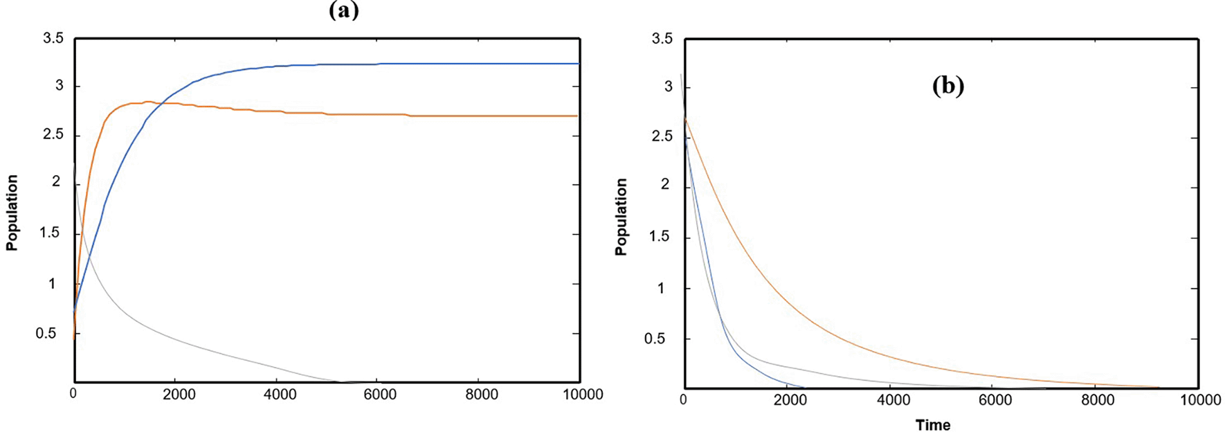
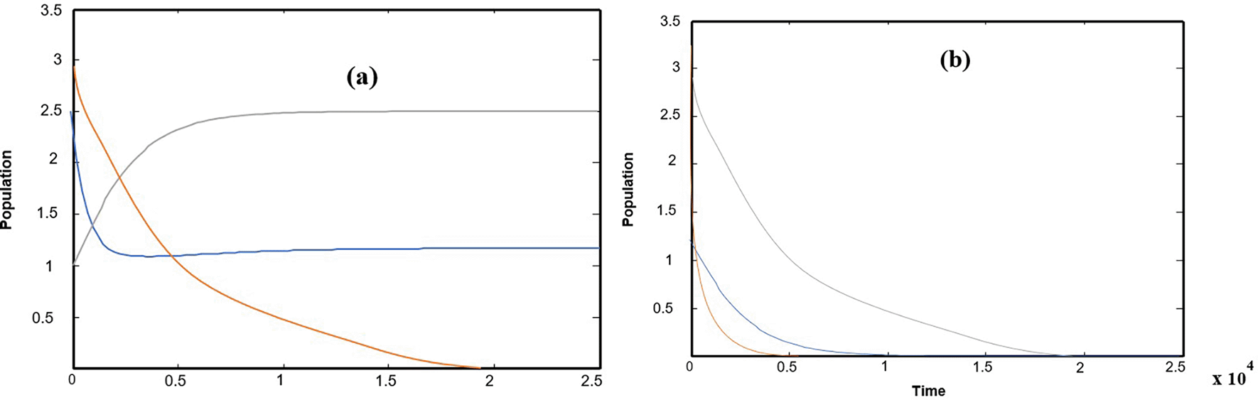
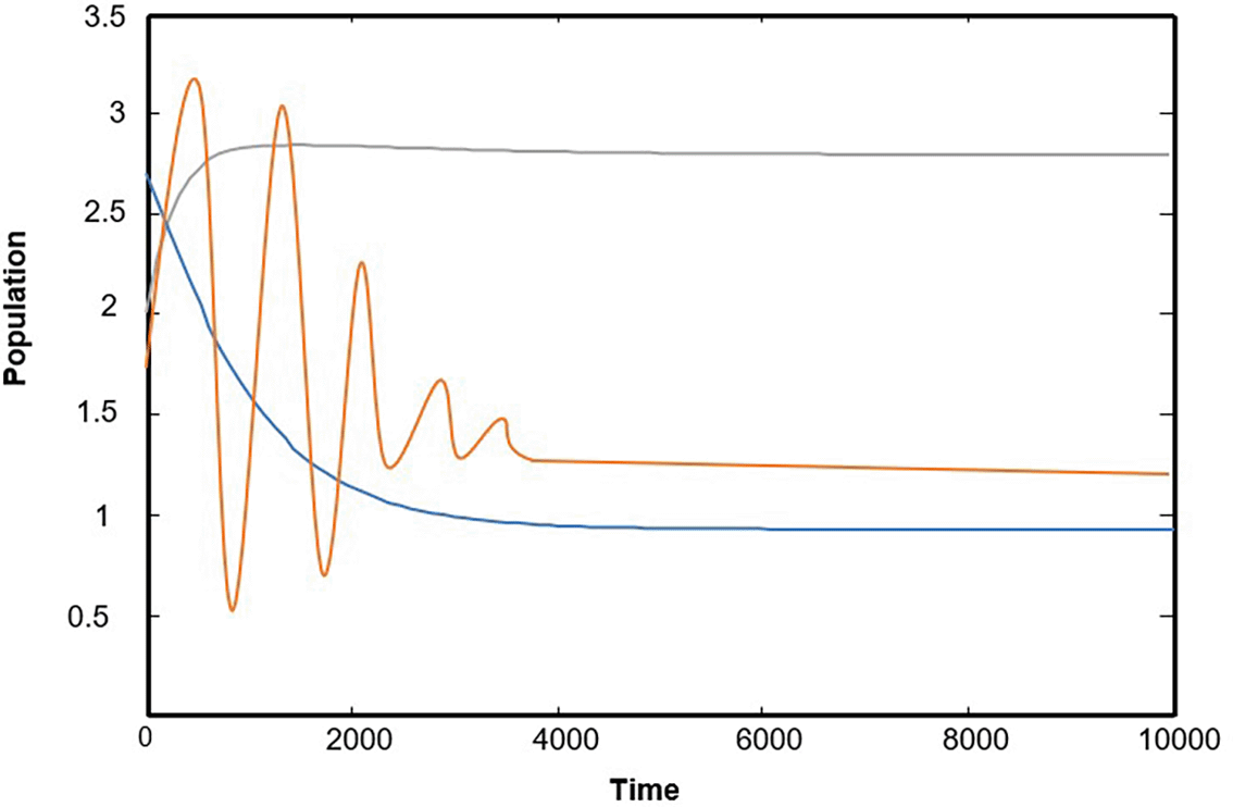
Numerical solutions using numerical software programs confirm the solution and provide an important interpretation for each point along the solution path (the equilibrium points of the system). We relied on the numerical solution using plotting programs in (matlab) and (C++), and the results were completed after providing approximate values for the key parameters in the system of differential equations. In the numerical interpretation of the paths and changes that occur in dynamics and stability, we show the stages of change that occur in the ecological community over time. As shown in Figure 1 that the population growth of the community (whether predator or prey) exhibits a state of global stability with more than one equilibrium point, and the results are convergent. This explains why predation by the predator is natural, and the population density in the prey community has caused it to grow naturally and steadily ( Figures (a), (b), and (c)), which clearly represents ecological sustainability; however, if we observe Figures 2, 3, and 4, we will see in each Figure that there is a complete absence and decline of one of the main ecological communities in the model, and this situation indicates that the increase in the predator community is the reason for the complete absence and predation of all organisms present in one of the other two types of prey communities. Likewise, Figures 5 and 6 show that in the community, there is only one organism that is still present in its ecological community: the prey organism. The complete absence of the predator in this case can be explained by the scarcity of its food and the intensity of competition within its ecological community. As for the last drawing, which is drawing Figure 7 it represents environmental evidence of the presence of the three organisms in the environment, complete stability in society, balance, and global convergence resulting from the availability of conditions for environmental coexistence, food sources for prey, and the abundance of sufficient food for predatory animals. All Figures are drawn to provide values for the parameters, and these values are approximate, as shown in the following sequence:

(32)

\begin{matrix} a_{1} = 0.6, b = 0.35, λ_{1} = 0.01, d_{1} = 0.015, a_{2} = 0.7, c = 0.4, λ_{2} = 0.02, d_{2} = 0.009, \\ e_{1} = 0.01, e_{2} = 0.03, d_{3} = 0.034, d_{4} = 0.022 . \end{matrix}}

Figure 1. The time series of the solution to model (1) which started from two different starting points (0.06, 0.12, 0.3) and (0.9, 0.4, 0.85) for the data in (32).

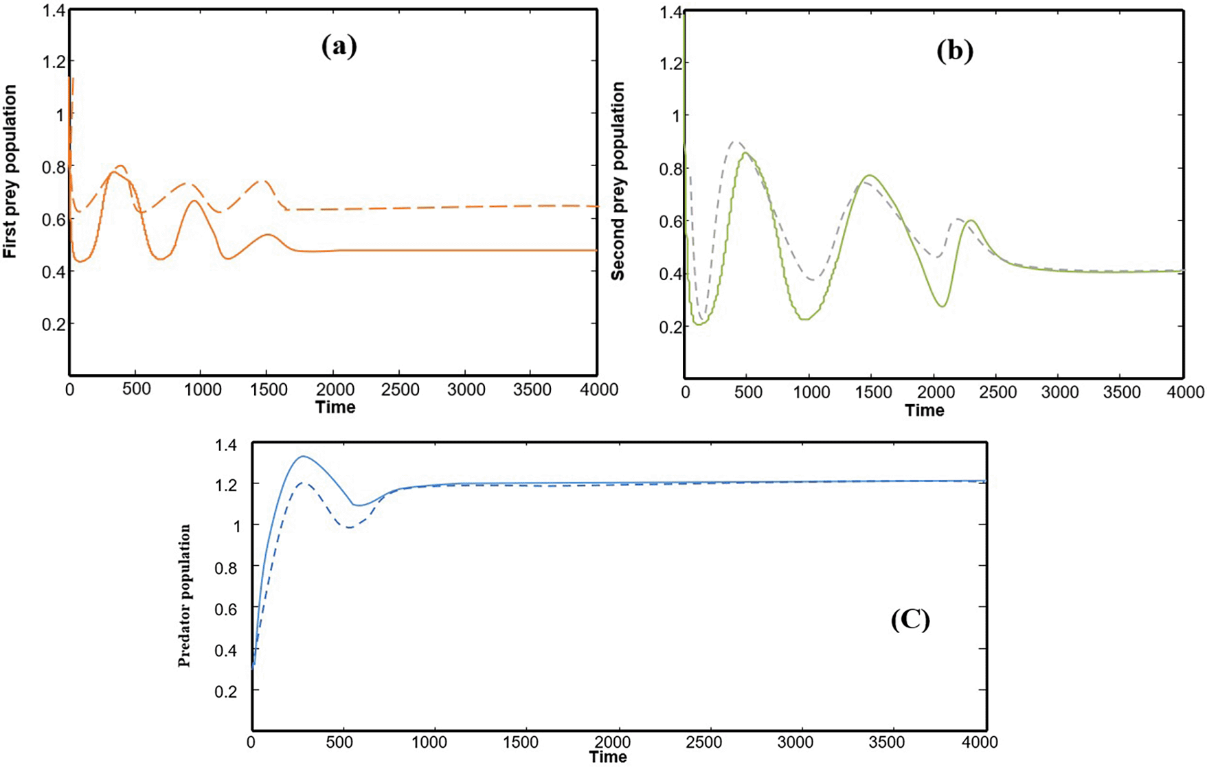
(a) Function of the time in which the path of the first prey is X, (b) Function of the time in which the path of the second prey is Y, (c) Function of the time in which the path of the predator is Z. Figure 1 express model (1) has an asymptotically of globally stable and the solution oncoming asymptotically point ${E_{6}}^{*} = (0.137,0.0125,0.031)$ asymptotically from starting tow initial of different points.

Figure 2. Time series of the solution of model (1) for data contained in (32) with ( $b =$ 0.5 and $c =$ 0.6), which oncoming to ${\tilde{E}}_{3} =$ (0.235,0.074,0) in R₊³.

Figure 3. (a) Time series of the solution of model (1) for data contained in (32) with $λ_{2} =$ 0.095 which oncoming to ${\overset{̿}{E}}_{5} = (0.632,0, 0.451)$ in the interior of R₊³ and (b) time series of the solution of model (1) for data contained in (32) with $λ_{2} =$ 0.7 which oncoming to $E_{0} = (0, 0, 0)$ in the interior of R₊³.

Figure 4. (a) Time series of the solution of model (1) for data contained in (32) with $λ_{1} =$ 0.031 which oncoming to ${\dot{E}}_{4} = (0,0.329,0.651)$ in the interior of R₊³ and (b) time series of the solution of model (1) for data contained in (32) with $λ_{1} =$ 0.527 which oncoming to $E_{0} = (0, 0, 0)$ in the interior of R₊³.

Figure 5. Time series of the solution of model (1) for data contained in (32) with $a_{2} = 1.25$ which oncoming to ${\bar{E}}_{2} = (0,0.832,0)$ in the interior of R₊³.

Figure 6. Time series of the solution of model (1) for data contained in (32) with $a_{1} = 1.4$ which oncoming to ${\hat{E}}_{1} = (0.451,0, 0)$ in the interior of R₊³.

Figure 7. Time series of the solution of model (1) for data contained in (32) with $e_{1} =$ 0.06 which oncoming to ${E_{6}}^{*} = (0.358,0.592, 0.071)$ in the interior of R₊³. This represents clear evidence of the sustainability and ecological balance achieved for the three organisms by maintaining the specified standards and taking into account the increase in natural food in parallel with the organisms that were considered prey, which led to an increase and balance in the predator’s food.

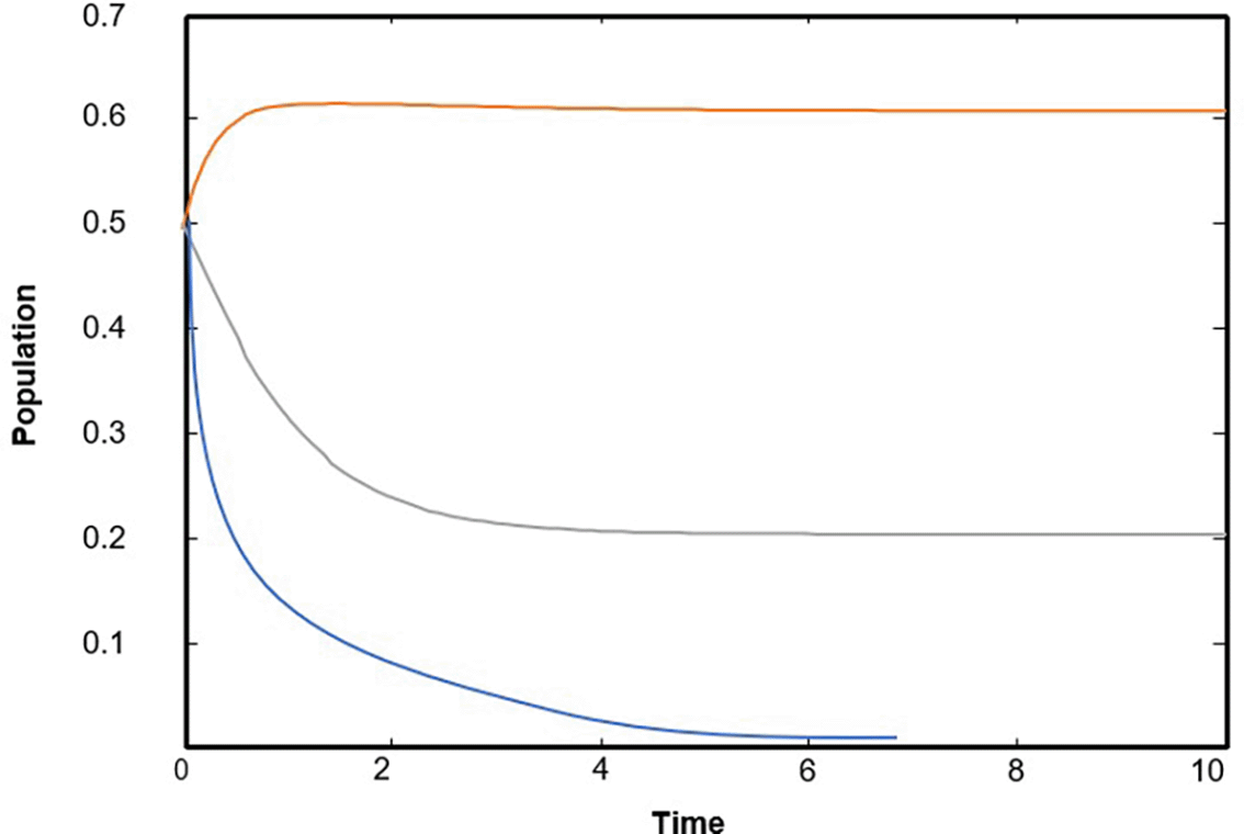
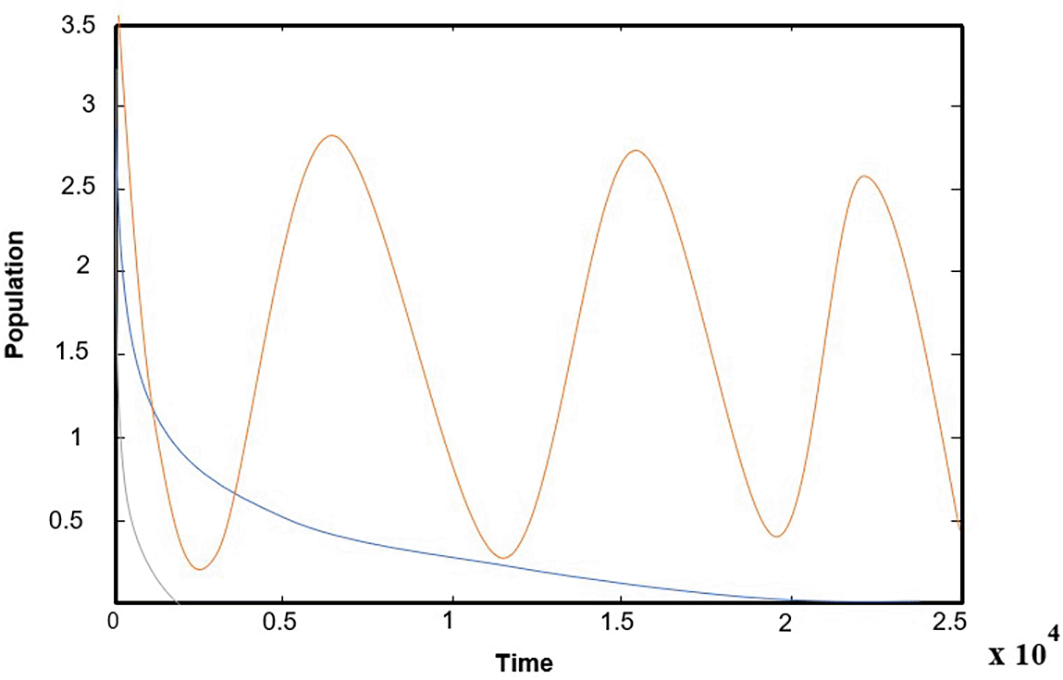
The varying of commensal relationship between the first prey X and the second prey Y in the intervals $(0.3 \leq b < 1.5$ and $0.2 \leq c < 1.8$ ) the rest of parameters are keeping as data in (32) observed that the model (1) has a solution which is approaches as asymptotically to ${\tilde{E}}_{3}$ , as shown in Figure 2, for typical value ( $b =$ 0.5 and $c =$ 0.6).

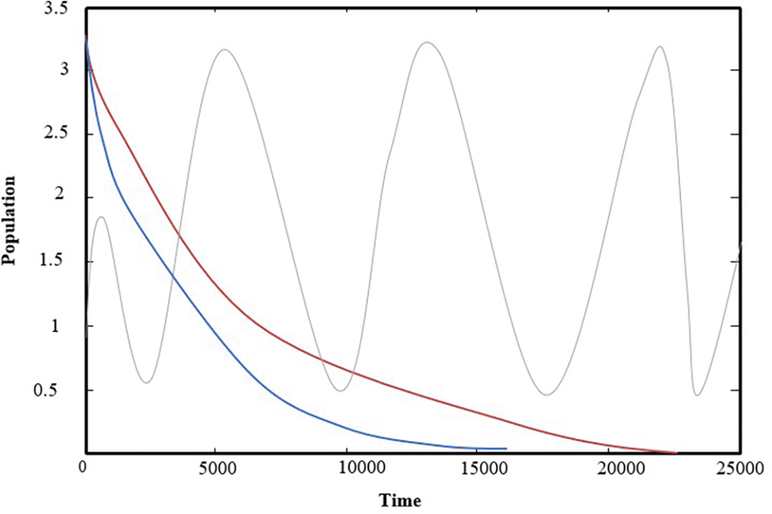
Now, varying the predator’s attack rate on the second prey $λ_{2}$ and the break of factors are kept as data take in (32). it is notice for 0.08 ≤ $λ_{2} < 0.651$ the solution of (1) approaches ${\overset{̿}{E}}_{5}$ , as shown in Figure 3(a), for typical1value $λ_{2}$ = 0.095, if we increase the parameter to 0.651 ≤ $λ_{2} < 0.942$ , it is observed that system (1) asymptotically approaches $E_{0},$ So $λ_{2}$ = 0.651 is a bifurcation point, as shown in Figure 3(b), for typical1value $λ_{2}$ = 0.7.

The change parameter $λ_{1}$ , represent the predator’s attack rate on the first prey, and the break of Factors are kept as data take in (32), it is noticed that for 0.003 ≤ $λ_{1} < 0.082$ the system (1) has a solution approaching ${\dot{E}}_{4}$ as shown in Figure 4(a) for typical1value $λ_{1} = 0.031,$ if we increasing the parameter for $0.082$ ≤ $λ_{1} < 0.725$ , it is observed that system (1) asymptotically approaches $E_{0},$ So $λ_{1}$ = $0.082$ is a bifurcation point, as shown in Figure 4(b), for typical1value $λ_{1}$ = 0.527.

The effect of the natural growth rate of the second prey $(a_{2})$ in the interval $0.17 \leq a_{2} < 2$ and the rest of the parameters are kept as data in (32), system (1) has a solution that asymptotically approaches as asymptotically to ${\bar{E}}_{2}$ , as shown in Figure 5, for a typical value $a_{2} = 1.25$ .

The effect of the natural growth rate of the first prey $(a_{1})$ in the interval $0.2 \leq a_{1} < 3$ and the rest of the parameters are kept as data in (32), system (1) has a solution that asymptotically approaches as asymptotically to ${\hat{E}}_{1}$ , as shown in Figure 6, for a typical value $a_{1} = 1.4$ .

The change of the parameter $(e_{1})$ , the rate of Food conversion from first prey to predator, and the break of Factors are keeping as data take in (32) it is notice for 0.05 ≤ $e_{1}$ < 0.2 the system (1) have a solution approaches $({E_{6}}^{*}),$ if we increase the parameter for $0.2$ ≤ $e_{1} < 0.92$ , it is observed that the system (1) asymptotically as approaches to ${\dot{E}}_{4}$ which has already been drawn above $,$ So $e_{1}$ = $0.2$ is a bifurcation point as shown in Figure 7, for typical1value $e_{1}$ = 0.06.

The change of the parameter $(e_{2})$ , the rate of Food conversion from second prey to predator, and the break of Factors are keeping as data take in (32) it is notice for 0.03 ≤ $e_{2}$ < 0.15 the system (1) have a solution approaches $({E_{6}}^{*}),$ if we increase the parameter for 0.15 ≤ $e_{2} < 1$ , it is observed that the system (1) asymptotically as approaches to ${\overset{̿}{E}}_{5} which has already been drawn above,$ so $e_{2}$ = $0.15$ is a bifurcation point.

The effect of the parameters $(d_{1}, d_{2}, d_{3}, d_{4})$ the natural rate of death for the three organisms, which are the first prey, the second prey, their predator, and the competition within the predator community, respectively, at all times, and the rest of the parameter keeping as data in (32), there is no effect on the dynamics of the behavior of model (1) and model (1) have a solution approach to ${E_{6}}^{*} .$

Conclusion with Discussion

This study aimed to draw conclusions from an equilibrium model of an ecosystem consisting of three organisms. A predator that feeds on the other two organisms, which have a positive relationship with survival and growth, is the primary food source for the predator. Predation (attack) by a predator on both prey depends on the first type of Holling functional response as a function of predation. In addition to what has been presented, and using numerical, analytical, and simulation methods, it has become clear that the natural growth or self-growth of both prey species plays an important role in ecological balance. Their mutual support also leads to a positive exchange of benefits, and reduces the risk of extinction in the face of continuous predation. In other words, the ecosystem will not collapse if the coexistence relationship continues. Therefore, the percentage of natural death and competition that occurs within the predator community must be on a curve parallel to the percentage that occurs within the community of the two prey, as the two prey are assumed to have competition and natural death within the same community, and these percentages make the system have a balanced natural growth rate that does not harm the prey as long as the curve between them and the predators is parallel. The effects of all parameters are studied numerically on the dynamic behavior of system (1), and the trajectories in the typical figures that represent the solutions and according to the solutions of system (1) for the data given by (32), the conclusions are obtained.

1- Model (1) does not have periodic dynamics for the data set, as given in (32).
2- The variations in the values of the set parameters in Equation (32), model (1) asymptotically approaches the globally stable point, ${E_{6}}^{*} = (0.137,0.0125,0.031)$ .
3- The effect of the parameters $(d_{1}, d_{2}, d_{3}, d_{4})$ the natural rate of death for the three organisms, which are the first prey, the second prey, their predator, and the competition within the predator community, respectively, at all times, and the rest of the parameter keeping as data in (32), there is no effect on the dynamics of the behavior of model (1) and model (1) have a solution approach to ${E_{6}}^{*} .$
4- The effect of the natural growth rate of the first prey $(a_{1})$ in the interval $(0.2 \leq a_{1} < 3)$ and the rest of the parameters are kept as data in (32) observed that system (1) has a solution that asymptotically approaches as asymptotically to ${\hat{E}}_{1}$ .
5- The effect of the natural growth rate of the second prey $(a_{2})$ in the interval $(0.17 \leq a_{2} < 2)$ and the rest of the parameters are kept as data in (32) observed that system (1) has a solution that asymptotically approaches as asymptotically to ${\bar{E}}_{2}$ .
6- The change parameter $λ_{1}$ represents the predator’s attack rate on the first prey, and the break of factors is kept as data take in (32); for 0.003 ≤ $λ_{1} < 0.082$ the system (1) has a solution approaching to ${\dot{E}}_{4}$ if we increase the parameter for $0.082$ ≤ $λ_{1} < 0.725$ , it is observed that system (1) asymptotically approaches $E_{0},$ So $λ_{1}$ = $0.082$ is a bifurcation.
7- Varying the predator’s attack rate on the second prey $λ_{2}$ and the break of factors are kept as data are taken in (32), it is notice for 0.08 ≤ $λ_{2} < 0.651$ the solution of (1) approaches to ${\overset{̿}{E}}_{5}$ , if we increasing the parameter for 0.651 ≤ $λ_{2} < 0.942$ , it is observed that the system (1) asymptotically as approaches to $E_{0},$ So $λ_{2}$ = 0.651 is a bifurcation point.
8- The effect of the commensal relationship between the first prey X and the second prey Y in the intervals $(0.3 \leq b < 1.5$ and $0.2 \leq c < 1.8$ ), the rest of the parameters are kept as data in (32) observed that model (1) has a solution that approaches asymptotically to ${\tilde{E}}_{3}$ .
9- The change of the parameter $(e_{1})$ , the rate of Food conversion from first prey to predator, and the break of Factors are keeping as data take in (32) it is notice for 0.05 ≤ $e_{1}$ < 0.2 the system (1) have a solution approaches $({E_{6}}^{*}),$ $,$ if we increase the parameter for $0.2$ ≤ $e_{1} < 0.92$ , it is observed that the system (1) asymptotically as approaches to ${\dot{E}}_{4},$ So $e_{1}$ = $0.2$ is a bifurcation point.
10- Finally, the change in parameter $(e_{2})$ , the rate of food conversion from second prey to predator, and the break of Factors are kept as data taken in (32). It is noticed that for 0.03 ≤ $e_{2}$ < 0.15, system (1) has a solution approach $({E_{6}}^{*}),$ if we increase the parameter for 0.15 ≤ $e_{2} < 1$ , it is observed that system (1) asymptotically approaches ${\overset{̿}{E}}_{5},$ so $e_{2}$ = $0.15$ is a bifurcation point.

Ethics and consent

Ethical consent was not required for this study.

Data availability

This study relies on numerical data generated from the proposed mathematical model. This data includes initial coefficients, initial conditions, and numerical simulation outputs (tables and figures). All of this data is not derived from field measurements but was generated programmatically for the purposes of theoretical analysis and numerical simulation of the system under study. This aligns with the general trend of sharing research data to enhance replication and reuse within the scientific community.

References

1. Fraser: Environmental Sustainability: Practical Global Applications. CRC Publishing; February 5, 2020. 978-1-4200-4874-2. Archived from the original on September 28, 2020.
2. Larry, Stewart R, Dietz T: Foundations of Environmental Sustainability. Oxford University Press; June 5, 2008. 978-0-19-530945-4. Archived from the original on 2020-09-28.
3. Ghosh B, Barman B, Saha M: Multiple dynamics in a delayed predator-prey model with asymmetric functional and numerical responses math. Methods Appl. Sci. 2023; 46: 5187–5207. Publisher Full Text
4. Xiang C, Huang J, Wang H: Bifurcations in Holling-Tanner model with generalist predator and prey refuge. J. Differ. Equ. 2023; 343: 495–529. Publisher Full Text
5. Keissar O, Scharf I, Sadeh A: Predator modulation of plant pathogen spread through induced changes in vector development rates. Ecological Entomology. 2020; 45(2): 213–222. Publisher Full Text
6. Greenhalgh D, Khan QJA, Al-Kharousi FA: Eco-epidemiological model with fatal disease in the prey. Nonlinear Analysis: Real World Applications. 2020; 53. Publisher Full Text
7. Cojocaru MG, Migot T, Jaber A: Controlling infection in predator-prey systems with transmission dynamics. Infectious Disease Modelling. 2020; 5: 1–11. PubMed Abstract | Publisher Full Text | Free Full Text
8. Al Themairi A, Alqudah MA: Predator-prey model of Holling-type II with harvesting and predator in disease. Italian journal of pure and applied mathematics. 2020; 43: 744–753.
9. Chen XH, Chen F: The influence of fear effect to a discrete-time predator-prey system with predator has other food resource. Mathematics. 2021; 9(8): 865. Publisher Full Text
10. Meng XY, Wu YQ, Li J: Bifurcation analysis of a singular nutrient- plankton-fish model with taxation, protected zone and multiple delays. Numerical Algebra, Control & Optimization. 2020; 10(3): 391. Publisher Full Text
11. Rani R, Gakkhar S, Moussaoui A: Dynamics of a fishery system in apatchy environment with nonlinear harvesting. Mathematical Methods in the Applied Sciences. 2019; 42(18): 7192–7209. Publisher Full Text
12. Yavuz M, Sene N: Stability analysis and numerical computation of the fractional predator–prey model with the harvesting rate. Fractal and Fractional. 2020; 4(3): 35. Publisher Full Text
13. Moustafa M, Mohd MH, Ismail AI, et al.: Dynamical analysis of a fractional-order eco-epidemiological model with disease in prey population. Advances in Difference Equations. 2020; 2020(1). Publisher Full Text
14. Yang R, Wang F, Jin D: Spatially inhomogeneous bifurcating periodic solutions induced by nonlocal competition in a predator–prey system with additional food. Mathematical Methods in the Applied Sciences. 2022; 45(16): 9967–9978. Publisher Full Text
15. Jawad MA, Ibrahim WA, Al-Qaisi SJM: Mixed Crank–Nicolson and Galerkin methods for solving nonlinear partial differential equation. Mustansiriy Journal of Pure and Applied Sciences. 2024; 2(4): 7–18. Publisher Full Text
16. Liu H, Yu H, Dai C, et al.: Dynamical analysis of an aquatic amensalism model with non-selective harvesting and Allee effect. Math. Biosci. Eng. 2021; 18(6): 8857–8882. PubMed Abstract | Publisher Full Text
17. Djilali S: Pattern formation of a diffusive predator-prey model with herd behavior and nonlocal prey competition. Math. Methods Appl. Sci. 2020; 43: 2233–2250. Publisher Full Text
18. Liu T, Chen L, Chen F, et al.: Dynamics of a Leslie-Gower Model withWeak Allee Effect on Prey and Fear Effect on Predator. Int. J. Bifurc. Chaos. 2023; 33: 2350008. Publisher Full Text
19. Kumar A, Dubey B: Dynamics of prey-predator model with strong and weak allee effect in the prey with gestation delay. Nonlinear Analysis: Modelling and Control. 2020; 25(3): 417–442.
20. Sarkar A, Sk N, Pal S: Effect of seasonally forced noisy environment on aquatic prey–predator model with water level fluctuations. Chaos Interdiscip. J. Nonlinear Sci. 2022; 32: 093115. PubMed Abstract | Publisher Full Text
21. Qi H, Meng X, Hayat T, et al.: Bifurcation dynamics of a reaction-diffusion predator-prey model with fear effect in apredator-poisoned environment. Math. Methods Appl. Sci. 2022; 45: 6217–6254. Publisher Full Text
22. Debnath S, Majumdar P, Sarkar S, et al.: Global dynamics of a prey–predator model with Holling type III functional response in the presence of harvesting. J. Biol. Syst. 2022; 30(01): 225–260. Publisher Full Text
23. Pool R, Chandradeva N, Gkafas G, et al.: Transmission and predictors of burden of lungworms of the striped dolphin (Stenella coeruleoalba) in the western mediterranean. J. Wildl. Dis. 2020; 56(1): 186–191. Publisher Full Text
24. Ghanbari B, Günerhan H, Srivastava HM: An application of the Atangana-Baleanu fractional derivative in mathematical biology: A three-species predator-prey model. Chaos, Solitons Fractals. 2020; 138: 109910. Publisher Full Text
25. Batabyal S, Jana D, Lyu J, et al.: Explosive predator and mutualistic preys: A comparative study. Physica A: Statistical Mechanics and its Applications. 2020; 541: 123348. Publisher Full Text
26. Santra PK, Mahapatra GS, Phaijoo GR: Bifurcation and Chaos of a Discrete Predator-Prey Model with Crowley-Martin Functional Response Incorporating Proportional Prey Refuge. Math. Probl. Eng. 2020; 2020: 1–18. Publisher Full Text
27. Souna F, Belabbas M, Menacer Y: Complex pattern formations induced by the presence of cross-diffusion in a generalized predator-prey model incorporating the Holling type functional response and generalization of habitat complexity effect. Math.Comput. Simul. 2023; 204: 597–618. Publisher Full Text
28. Sk N, Pal S: Dynamics of an infected prey-generalist predator system with the effects of fear, refuge and harvesting: Deterministic and stochastic approach. Eur. Phys. J. Plus. 2022; 137: 138. Publisher Full Text
29. Mondal B, Ghosh U, Rahman MS, et al.: Studies of different types of bifurcations analyses of an imprecise two species food chain model with fear effect and non-linear harvesting. Math. Comput. Simul. 2022; 192: 111–135. Publisher Full Text
30. Ghanem H, Majeed AA: A qualitative study of an eco-epidemiological model with (SI) epidemic disease in prey and (SIS) epidemic disease in predator involving a harvesting.2018.
31. Ouahab A, Belabbas M, Henderson J, et al.: Existence and transportation inequalities for fractional stochastic differential equations. Turk. J. Math. 2022; 46: 710–727. Publisher Full Text
32. Hossain M, Pal S, Kumar Tiwari P, et al.: Bifurcations, chaos, and multi stability in a non-autonomous predator–prey model with fear. Chaos Interdiscip. J. Nonlinear Sci. 2021; 31: 123134. Publisher Full Text
33. Yousef FB, Yousef A, Maji C: Effects of fear in a fractional-order predator-prey system with predator density-dependent prey mortality. Chaos, Solitons Fractals. 2021; 145: 110711. Publisher Full Text
34. Ghanem H, Khaleefah K: A Dynamic Mathematical Model That Describes Predatory Fisheries In The Presence Of Harvester (Model Of Bioeconomic). Earth Environ. Sci. 2025; 1507: 012014. Publisher Full Text

Comments on this article Comments (0)

Version 1

VERSION 1 PUBLISHED 15 Dec 2025

Author details Author details

Department of Civil Techniques, Middle Technical University, Baghdad, Baghdad Governorate, Iraq

Haider Ghanem Sufaeh
Roles: Conceptualization, Data Curation, Formal Analysis, Funding Acquisition, Investigation, Methodology, Project Administration, Resources, Software, Supervision, Validation, Visualization, Writing – Original Draft Preparation, Writing – Review & Editing

Competing interests

No competing interests were disclosed.

Grant information

The author(s) declared that no grants were involved in supporting this work.

Article Versions (1)

version 1

Published: 15 Dec 2025, 14:1397

https://doi.org/10.12688/f1000research.172164.1

Copyright

© 2025 Ghanem Sufaeh H. This is an open access article distributed under the terms of the Creative Commons Attribution License, which permits unrestricted use, distribution, and reproduction in any medium, provided the original work is properly cited.

Download

Export To

metrics

	Views	Downloads
F1000Research	-	-
PubMed Central Data from PMC are received and updated monthly.	-	-

Citations

0

SEE MORE DETAILS

CITE

how to cite this article

Ghanem Sufaeh H. Using Mathematical Modeling in Environmental Sustainability to Study The Ecological Balance Between A Predator That Feeds on Two Types of Prey [version 1; peer review: awaiting peer review]. F1000Research 2025, 14:1397 (https://doi.org/10.12688/f1000research.172164.1)

NOTE: If applicable, it is important to ensure the information in square brackets after the title is included in all citations of this article.

track

receive updates on this article

Track an article to receive email alerts on any updates to this article.

Open Peer Review

Comments on this article Comments (0)

Version 1

VERSION 1 PUBLISHED 15 Dec 2025

Open Peer Review

Reviewer Status

AWAITING PEER REVIEW

Comments on this article

All Comments(0)

Add a comment

Sign up for content alerts

Browse by related subjects

[1] 1. Fraser: Environmental Sustainability: Practical Global Applications. CRC Publishing; February 5, 2020. 978-1-4200-4874-2. Archived from the original on September 28, 2020.

[2] 2. Larry, Stewart R, Dietz T: Foundations of Environmental Sustainability. Oxford University Press; June 5, 2008. 978-0-19-530945-4. Archived from the original on 2020-09-28.

[3] 3. Ghosh B, Barman B, Saha M: Multiple dynamics in a delayed predator-prey model with asymmetric functional and numerical responses math. Methods Appl. Sci. 2023; 46: 5187–5207. Publisher Full Text

[4] 4. Xiang C, Huang J, Wang H: Bifurcations in Holling-Tanner model with generalist predator and prey refuge. J. Differ. Equ. 2023; 343: 495–529. Publisher Full Text

[5] 5. Keissar O, Scharf I, Sadeh A: Predator modulation of plant pathogen spread through induced changes in vector development rates. Ecological Entomology. 2020; 45(2): 213–222. Publisher Full Text

[6] 6. Greenhalgh D, Khan QJA, Al-Kharousi FA: Eco-epidemiological model with fatal disease in the prey. Nonlinear Analysis: Real World Applications. 2020; 53. Publisher Full Text

[7] 7. Cojocaru MG, Migot T, Jaber A: Controlling infection in predator-prey systems with transmission dynamics. Infectious Disease Modelling. 2020; 5: 1–11. PubMed Abstract | Publisher Full Text | Free Full Text

[8] 8. Al Themairi A, Alqudah MA: Predator-prey model of Holling-type II with harvesting and predator in disease. Italian journal of pure and applied mathematics. 2020; 43: 744–753.

[9] 9. Chen XH, Chen F: The influence of fear effect to a discrete-time predator-prey system with predator has other food resource. Mathematics. 2021; 9(8): 865. Publisher Full Text

[10] 10. Meng XY, Wu YQ, Li J: Bifurcation analysis of a singular nutrient- plankton-fish model with taxation, protected zone and multiple delays. Numerical Algebra, Control & Optimization. 2020; 10(3): 391. Publisher Full Text

[11] 11. Rani R, Gakkhar S, Moussaoui A: Dynamics of a fishery system in apatchy environment with nonlinear harvesting. Mathematical Methods in the Applied Sciences. 2019; 42(18): 7192–7209. Publisher Full Text

[12] 12. Yavuz M, Sene N: Stability analysis and numerical computation of the fractional predator–prey model with the harvesting rate. Fractal and Fractional. 2020; 4(3): 35. Publisher Full Text

[13] 13. Moustafa M, Mohd MH, Ismail AI, et al.: Dynamical analysis of a fractional-order eco-epidemiological model with disease in prey population. Advances in Difference Equations. 2020; 2020(1). Publisher Full Text

[14] 14. Yang R, Wang F, Jin D: Spatially inhomogeneous bifurcating periodic solutions induced by nonlocal competition in a predator–prey system with additional food. Mathematical Methods in the Applied Sciences. 2022; 45(16): 9967–9978. Publisher Full Text

[15] 15. Jawad MA, Ibrahim WA, Al-Qaisi SJM: Mixed Crank–Nicolson and Galerkin methods for solving nonlinear partial differential equation. Mustansiriy Journal of Pure and Applied Sciences. 2024; 2(4): 7–18. Publisher Full Text

[16] 16. Liu H, Yu H, Dai C, et al.: Dynamical analysis of an aquatic amensalism model with non-selective harvesting and Allee effect. Math. Biosci. Eng. 2021; 18(6): 8857–8882. PubMed Abstract | Publisher Full Text

[17] 17. Djilali S: Pattern formation of a diffusive predator-prey model with herd behavior and nonlocal prey competition. Math. Methods Appl. Sci. 2020; 43: 2233–2250. Publisher Full Text

[18] 18. Liu T, Chen L, Chen F, et al.: Dynamics of a Leslie-Gower Model withWeak Allee Effect on Prey and Fear Effect on Predator. Int. J. Bifurc. Chaos. 2023; 33: 2350008. Publisher Full Text

[19] 19. Kumar A, Dubey B: Dynamics of prey-predator model with strong and weak allee effect in the prey with gestation delay. Nonlinear Analysis: Modelling and Control. 2020; 25(3): 417–442.

[20] 20. Sarkar A, Sk N, Pal S: Effect of seasonally forced noisy environment on aquatic prey–predator model with water level fluctuations. Chaos Interdiscip. J. Nonlinear Sci. 2022; 32: 093115. PubMed Abstract | Publisher Full Text

[21] 21. Qi H, Meng X, Hayat T, et al.: Bifurcation dynamics of a reaction-diffusion predator-prey model with fear effect in apredator-poisoned environment. Math. Methods Appl. Sci. 2022; 45: 6217–6254. Publisher Full Text

[22] 22. Debnath S, Majumdar P, Sarkar S, et al.: Global dynamics of a prey–predator model with Holling type III functional response in the presence of harvesting. J. Biol. Syst. 2022; 30(01): 225–260. Publisher Full Text

[23] 23. Pool R, Chandradeva N, Gkafas G, et al.: Transmission and predictors of burden of lungworms of the striped dolphin (Stenella coeruleoalba) in the western mediterranean. J. Wildl. Dis. 2020; 56(1): 186–191. Publisher Full Text

[24] 24. Ghanbari B, Günerhan H, Srivastava HM: An application of the Atangana-Baleanu fractional derivative in mathematical biology: A three-species predator-prey model. Chaos, Solitons Fractals. 2020; 138: 109910. Publisher Full Text

[25] 25. Batabyal S, Jana D, Lyu J, et al.: Explosive predator and mutualistic preys: A comparative study. Physica A: Statistical Mechanics and its Applications. 2020; 541: 123348. Publisher Full Text

[26] 26. Santra PK, Mahapatra GS, Phaijoo GR: Bifurcation and Chaos of a Discrete Predator-Prey Model with Crowley-Martin Functional Response Incorporating Proportional Prey Refuge. Math. Probl. Eng. 2020; 2020: 1–18. Publisher Full Text

[27] 27. Souna F, Belabbas M, Menacer Y: Complex pattern formations induced by the presence of cross-diffusion in a generalized predator-prey model incorporating the Holling type functional response and generalization of habitat complexity effect. Math.Comput. Simul. 2023; 204: 597–618. Publisher Full Text

[28] 28. Sk N, Pal S: Dynamics of an infected prey-generalist predator system with the effects of fear, refuge and harvesting: Deterministic and stochastic approach. Eur. Phys. J. Plus. 2022; 137: 138. Publisher Full Text

[29] 29. Mondal B, Ghosh U, Rahman MS, et al.: Studies of different types of bifurcations analyses of an imprecise two species food chain model with fear effect and non-linear harvesting. Math. Comput. Simul. 2022; 192: 111–135. Publisher Full Text

[30] 30. Ghanem H, Majeed AA: A qualitative study of an eco-epidemiological model with (SI) epidemic disease in prey and (SIS) epidemic disease in predator involving a harvesting.2018.

[31] 31. Ouahab A, Belabbas M, Henderson J, et al.: Existence and transportation inequalities for fractional stochastic differential equations. Turk. J. Math. 2022; 46: 710–727. Publisher Full Text

[32] 32. Hossain M, Pal S, Kumar Tiwari P, et al.: Bifurcations, chaos, and multi stability in a non-autonomous predator–prey model with fear. Chaos Interdiscip. J. Nonlinear Sci. 2021; 31: 123134. Publisher Full Text

[33] 33. Yousef FB, Yousef A, Maji C: Effects of fear in a fractional-order predator-prey system with predator density-dependent prey mortality. Chaos, Solitons Fractals. 2021; 145: 110711. Publisher Full Text

[34] 34. Ghanem H, Khaleefah K: A Dynamic Mathematical Model That Describes Predatory Fisheries In The Presence Of Harvester (Model Of Bioeconomic). Earth Environ. Sci. 2025; 1507: 012014. Publisher Full Text

Using Mathematical Modeling in Environmental Sustainability to Study The Ecological Balance Between A Predator That Feeds on Two Types of Prey

Abstract

Background

Methodology

Results

Conclusions

Keywords

Introduction

Formulation of mathematical model

(1)

Table 1. The parameters of the model (1).

Theorem 1:

Proof:

Existence of equilibrium points

(2)

(3)

(4)

(5)

(6)

(7)

(8)

Local stability analysis

(9)

(10)

(11)

(12)

(13)

(14)

(15)

(16)

(17)

(18)

(19)

(20)

(21)

(22)

(23)

Globally analysis

Lemma:

Theorem 2:

(24)

(25)

Proof:

Theorem 3:

(26)

(27)

Proof:

Theorem 4:

(28)

(29)

Proof:

Theorem 5:

(30)

(31)

Proof:

Numerical simulation

(32)

Figure 1. The time series of the solution to model (1) which started from two different starting points (0.06, 0.12, 0.3) and (0.9, 0.4, 0.85) for the data in (32).

Figure 2. Time series of the solution of model (1) for data contained in (32) with ( b= 0.5 and c= 0.6), which oncoming to E~3= (0.235,0.074,0) in R+3.

Figure 5. Time series of the solution of model (1) for data contained in (32) with a2=1.25 which oncoming to E¯2=(0,0.832,0) in the interior of R+3.

Figure 6. Time series of the solution of model (1) for data contained in (32) with a1=1.4 which oncoming to Ê1=(0.451,0,0) in the interior of R+3.

Conclusion with Discussion

Ethics and consent

Data availability

References

Comments on this article Comments (0)

Open Peer Review

Comments on this article Comments (0)

Open Peer Review

Reviewer Status

Comments on this article

Browse by related subjects

Competing Interests Policy

Stay Updated

Figure 2. Time series of the solution of model (1) for data contained in (32) with ( $b =$ 0.5 and $c =$ 0.6), which oncoming to ${\tilde{E}}_{3} =$ (0.235,0.074,0) in R₊³.

Figure 5. Time series of the solution of model (1) for data contained in (32) with $a_{2} = 1.25$ which oncoming to ${\bar{E}}_{2} = (0,0.832,0)$ in the interior of R₊³.

Figure 6. Time series of the solution of model (1) for data contained in (32) with $a_{1} = 1.4$ which oncoming to ${\hat{E}}_{1} = (0.451,0, 0)$ in the interior of R₊³.