An Iterative Approach for Solving Fractional Differential Equations Using the α-Generalized Daftardar–Jafari Method

Sahib Abdulkadhim Sachit; Hassan Kamil Jassim

doi:10.12688/f1000research.172333.1

Home Browse An Iterative Approach for Solving Fractional Differential Equations...

ALL Metrics

-

Views

-

Downloads

Get PDF

Get XML

Export

▬

✚

Research Article

An Iterative Approach for Solving Fractional Differential Equations Using the α-Generalized Daftardar–Jafari Method

[version 1; peer review: awaiting peer review]

Sahib Abdulkadhim Sachit ^1,2, Hassan Kamil Jassim¹

PUBLISHED 23 Dec 2025

Author details Author details

¹ Mathematics, University of Thi-Qar, An Nasiriyah, Dhi Qar, 64001, Iraq
² Technical Engineering, University of Science and Technology, An Nasiriyah, Dhi Qar, 64001, Iraq

Sahib Abdulkadhim Sachit
Roles: Formal Analysis, Investigation, Methodology, Writing – Original Draft Preparation

Hassan Kamil Jassim
Roles: Investigation, Supervision, Writing – Review & Editing

OPEN PEER REVIEW

REVIEWER STATUS AWAITING PEER REVIEW

This article is included in the Fallujah Multidisciplinary Science and Innovation gateway.

Abstract

Background

Fractional calculus has gained significant attention due to its applications in modeling complex systems. This paper introduces several fundamental fractional operators, including the Riemann–Liouville, Caputo, and Hadamard operators. From these, a novel α-generalized fractional operator is derived, which plays a crucial role in solving fractional partial differential equations (FPDEs).

Methods

The α-generalized operator is analytically constructed and its properties are rigorously proven. It is then integrated with the Daftardar–Jafari iterative method (DJM) to solve both linear and nonlinear FPDEs. The convergence of the proposed method is established using the Lipschitz condition. Two benchmark equations—the linear fractional Burger’s equation and the nonlinear fractional Heat-type equation—are used to demonstrate the method’s applicability. MATLAB is employed to implement the numerical schemes and visualize the results.

Results

The DJM combined with the α-generalized operator yields superior numerical results compared to the Adomian decomposition method. This superiority is evident in both accuracy and convergence, especially for the nonlinear fractional Heat-type equation. Tabulated results and graphical comparisons confirm the effectiveness of the proposed approach across different values of α.

Conclusions

The integration of the α-generalized operator with the Daftardar–Jafari method provides a powerful tool for solving FPDEs. Its numerical advantages make it a promising alternative to existing methods. The study recommends extending this framework to other fractional operators, iterative schemes, and potential transformation techniques, with applications in quantum physics, fluid dynamics, and beyond.

Keywords

Adomian Decomposition Method, Daftardar–Jafari iterative method, Generalized fractional derivative (α-operator), Fractional partial differential equations, Existence and uniqueness, Heat-type equation, Burger’s equation.

Corresponding author: Sahib Abdulkadhim Sachit

Competing interests: No competing interests were disclosed.

Grant information: The author(s) declared that no grants were involved in supporting this work.

Copyright: © 2025 Abdulkadhim Sachit S and Kamil Jassim H. This is an open access article distributed under the terms of the Creative Commons Attribution License, which permits unrestricted use, distribution, and reproduction in any medium, provided the original work is properly cited.

How to cite: Abdulkadhim Sachit S and Kamil Jassim H. An Iterative Approach for Solving Fractional Differential Equations Using the α-Generalized Daftardar–Jafari Method [version 1; peer review: awaiting peer review]. F1000Research 2025, 14:1437 (https://doi.org/10.12688/f1000research.172333.1) First published: 23 Dec 2025, 14:1437 (https://doi.org/10.12688/f1000research.172333.1) Latest published: 23 Dec 2025, 14:1437 (https://doi.org/10.12688/f1000research.172333.1)

1. Introduction

Over the past decades, fractional calculus has emerged as a powerful generalization of classical differentiation and integration. It has found applications across a wide spectrum of disciplines. Its origins trace back to a 1695 correspondence, in which Leibniz proposed the concept of a half-order derivative in his letter to L’Hôpital. Since that seminal insight, fractional operators have attracted the interest of mathematicians, physicists, biologists, engineers, and economists.

One of the earliest celebrated applications appears in Abel’s resolution of the tautochrone problem.¹ In modern research, fractional models play a central role in various fields. These include biophysics, quantum mechanics, wave propagation, polymer dynamics, continuum mechanics, Lie group analysis, field theory, and spectroscopy.^2–8 For a comprehensive treatment of these developments, see Samko et al.⁹

Over time, many formulations of the fractional derivative have been introduced. These include the Riemann–Liouville, Caputo, Hadamard, Erdélyi–Kober, Grünwald–Letnikov, Machado, and Riesz definitions. Each formulation addresses distinct theoretical and practical challenges.^8–12

In fractional calculus, derivatives of non-integer order are most often introduced via fractional integrals.^10,11 The Riemann–Liouville operator and its associated integral occupy a foundational role in the theory.¹³ The widely used Caputo derivative is itself defined through the Riemann–Liouville integral.⁹

In parallel, Butzer and colleagues have conducted extensive studies on the Hadamard fractional integral and derivative.^{10,11,14–18} They derived, in particular, the Mellin transform representation of these operators.¹⁵

More recently, Pooseh et al. established expansion formulas that express Hadamard operators in terms of standard integer-order derivatives.¹⁹ For further developments and a comprehensive survey of related results, see Samko et al.,¹⁰ Srivastava et al.,¹¹ and the references therein.

In Ref. 12, a new fractional integral was introduced. It unifies the Riemann–Liouville and Hadamard integrals within a single formulation. This α-generalized operator has been the subject of numerous recent studies and monographs.^18,20–24

The first part of this paper reviews the essential concepts and definitions of fractional calculus that underpin our framework. The second part presents rigorous proofs of existence and uniqueness for the generalized α-operator. In the third part, we develop a detailed analysis of the Daftardar-Jafari iterative method when combined with this operator. The fourth part illustrates the applicability of both the operator and the method through several example problems in fractional differential equations.

Finally, we draw conclusions and compile a complete list of references.

2. Preliminaries

Definition 1.

⁹ The Riemann Liouville fractional integral operator of order $α \geq 0,$ of function $φ (τ)$ is defined as

(1)

I_{τ}^{α} φ (τ) = {\begin{matrix} \frac{1}{Γ (α)} \int_{0}^{τ} {(τ - s)}^{α - 1} φ (s) ds, & α > 0 . τ > 0 \\ φ (τ), & α = 0 \end{matrix},

where

Γ (∙)

is the well-known Gamma function

Definition 2.

⁹ The Liouville-Caputo operator (c) with order $(α > 0)$ of $φ (τ)$ is defined as follows:

(2)

{}^{c}D_{τ}^{α} φ (τ) = {\begin{matrix} \frac{1}{Γ (m - α)} \int_{0}^{τ} {(τ - s)}^{m - α - 1} φ^{(m)} (s) ds, & m - 1 < α \leq m \\ \frac{\partial^{n}}{\partial τ^{n}} φ (τ), & α = n \in ℕ \end{matrix},

Definition 3.

¹¹ The Hadamard fractional integral introduced by J. Hadamard,¹¹ and is given by,

(3)

I_{a^{+}}^{α, ρ} φ (τ) = \frac{1}{Γ (α)} \int_{a}^{τ} {(log \frac{τ}{t})}^{α - 1} φ (t) \frac{dt}{t} .

For $Re (α) > 0, τ > a \geq 0$ while the Hadamard fractional derivative of order $α \in ℂ, Re (α) > 0$ is given by,

(4)

D_{a^{+}}^{α} φ (τ) = {(τ \frac{d}{dτ})}^{n} \frac{1}{Γ (n - α)} \int_{a}^{τ} {(log \frac{τ}{t})}^{n - α - 1} φ (t) \frac{dt}{t} .

Definition 4.

¹³ The α‐generalized fractional derivative operator of order $0 < α < 1, τ > 0, ρ$ is constant of function $φ (τ) \in ∁_{ε}, ε \geq - 1$ is defined as

(5)

{}_{0}D_{τ}^{α, ρ} φ (τ) = \frac{ρ^{α}}{Γ (1 - α)} τ^{1 - ρ} \frac{d}{dτ} \int_{0}^{τ} {(τ^{ρ} - t^{ρ})}^{- α} t^{ρ - 1} φ (t) dt,

while the α‐generalized fractional integral operator²⁵ of order

0 < α < 1, τ > 0, ρ

is constant of function

φ (τ)

is defined as

(6)

({}^{ρ}{I_{a +}^{α}} φ) (τ) = \frac{ρ^{1 - α}}{Γ (α)} \int_{a}^{τ} {(τ^{ρ} - t^{ρ})}^{α - 1} t^{ρ - 1} φ (t) dt .

Theorem 1.

²⁶ Let $α ϵ ℂ, Re (α) \geq 0, n = ⌈ Re (α) ⌉ and ρ > 0 . Then, for x > a,$

(7)

lim_{ρ \to 1} D_{τ}^{α, ρ} φ (τ) = {(\frac{d}{dτ})}^{n} \frac{1}{Γ (n - α)} \int_{0}^{τ} {(τ - t)}^{n - α - 1} φ (t) dt,

(8)

lim_{ρ \to 0^{+}} D_{τ}^{α, ρ} φ (τ) = {(τ \frac{d}{dτ})}^{n} \frac{1}{Γ (n - α)} \int_{a}^{τ} {(log \frac{τ}{t})}^{n - α - 1} φ (t) \frac{dt}{t},

(9)

lim_{ρ \to 1} {}^{ρ}{I_{a +}^{α}} φ (τ) = \frac{1}{Γ (α)} \int_{a}^{τ} {(τ - t)}^{α - 1} φ (t) dt,

(10)

lim_{ρ \to 0 +} {}^{ρ}{I_{a +}^{α}} φ (τ) = \frac{1}{Γ (α)} \int_{a}^{τ} {(log \frac{τ}{t})}^{α - 1} φ (t) \frac{dt}{t} .

Proof.

This result was originally established in Ref. 26, to which we refer the reader for the full proof. This result was originally established in Ref. 26, to which we refer the reader for the full proof.

Theorem 2.

Let $0 < α < 1, φ (τ) \in X_{c}^{p} (a, b), a > 0, and ρ > 0$ . Then

(11)

(D_{a +}^{α, ρ} {}^{ρ}{I_{a +}^{α}}) φ (τ) = φ (τ) .

Proof.

(12)

\begin{matrix} (D_{a +}^{α, ρ} {}^{ρ}{I_{a +}^{α}}) φ (τ) \\ = \frac{ρ^{α}}{Γ (1 - α)} τ^{1 - ρ} \frac{d}{dτ} \int_{a}^{τ} {(τ^{ρ} - t^{ρ})}^{- α} t^{ρ - 1} \frac{ρ^{1 - α}}{Γ (α)} \int_{a}^{t} {(t^{ρ} - x^{ρ})}^{α - 1} x^{ρ - 1} φ (x) dx dt . \end{matrix}

By using Fubini’s theorem, the equation will become as follows,

(13)

= \frac{ρ}{Γ (1 - α) Γ (α)} τ^{1 - ρ} \frac{d}{dτ} \int_{a}^{τ} x^{ρ - 1} φ (x) dx \int_{x}^{τ} {(τ^{ρ} - t^{ρ})}^{- α} {(t^{ρ} - x^{ρ})}^{α - 1} t^{ρ - 1} dt .

By employing an appropriate substitution of variables,

(14)

y = \frac{(t^{ρ} - x^{ρ})}{(τ^{ρ} - x^{ρ})},

(15)

\begin{matrix} y \to 1, when t ⟶ τ, and y ⟶ 0, when t ⟶ x \\ (t^{ρ} - x^{ρ}) = y (τ^{ρ} - x^{ρ}), \end{matrix}

(16)

t^{ρ} = x^{ρ} + y (τ^{ρ} - x^{ρ}),

(17)

ρ t^{ρ - 1} dt = (τ^{ρ} - x^{ρ}) dy,

(18)

t^{ρ - 1} dt = \frac{(τ^{ρ} - x^{ρ})}{ρ} dy .

Substitution Eq. (16) and Eq. (18) in Eq. (13):

(19)

= \frac{ρ}{Γ (1 - α) Γ (α)} τ^{1 - ρ} \frac{d}{dτ} \int_{a}^{τ} x^{ρ - 1} φ (x) dx \int_{0}^{1} {(τ^{ρ} - x^{ρ} - y (τ^{ρ} - x^{ρ}))}^{- α} {(x^{ρ} + y (τ^{ρ} - x^{ρ}) - x^{ρ})}^{α - 1} \frac{(τ^{ρ} - x^{ρ})}{ρ} dy .

(20)

= \frac{ρ}{Γ (1 - α) Γ (α)} τ^{1 - ρ} \frac{d}{dτ} \int_{a}^{τ} x^{ρ - 1} φ (x) dx \frac{{(τ^{ρ} - t^{ρ})}^{- α + α - 1 + 1}}{ρ} \int_{0}^{1} {(1 - y)}^{- α} y^{α - 1} dy .

Using the Beta function, we have

(21)

= \frac{ρ}{Γ (1 - α) Γ (α)} τ^{1 - ρ} \frac{d}{dτ} \int_{a}^{τ} x^{ρ - 1} φ (x) dx . \frac{Γ (1 - α) Γ (α)}{ρ},

(22)

= τ^{1 - ρ} \frac{d}{dτ} \int_{a}^{τ} x^{ρ - 1} φ (x) dx .

Applying Leibniz’s rule

(23)

(D_{a +}^{α, ρ} {}^{ρ}{I_{a +}^{α}}) φ (τ) = φ (τ) .

Theorem 3.

Let $α, σ \in ℂ$ such that $0 < Re (α)$ and $Re (σ) < 1 .$ If $0 < a < b < \infty$ and $1 \leq ρ \leq \infty$ , then, for $φ (τ) \in X_{c}^{p} (a, b), ρ > 0$

(24)

[{}^{ρ}{I_{a +}^{α}} {}^{ρ}{I_{a +}^{σ}}] φ (τ) = {}^{ρ}{I_{a +}^{α + σ}} φ (τ), and (D_{a +}^{α, ρ} D_{a +}^{σ, ρ}) φ (τ) = D_{a +}^{α + σ, ρ} φ (τ) .

Proof.

This result was originally established in Ref. 27, to which we refer the reader for the full proof.

Theorem 4.

Let $α \in ℂ such that 0 < Re (α) < 1 . If 0 < a < b < \infty and 1 \leq ρ \leq \infty, then, for φ, ψ \in X_{c}^{p} (a, b), ρ > 0$

(25)

{}^{ρ}{I_{a +}^{α}} (φ + ψ) = {}^{ρ}{I_{a +}^{α}} φ + {}^{ρ}{I_{a +}^{α}} ψ, and D_{a +}^{α, ρ} (φ + ψ) = D_{a +}^{α, ρ} φ + D_{a +}^{α, ρ} ψ .

It is easy to prove this theorem, which is called the linear property theorem.

Proposition 1.

For $0 < α < 1$ and $ρ \in ℝ,$ then

(26)

D_{a +}^{α, ρ} τ^{n} = ρ^{α} \frac{Γ (\frac{n}{ρ} + 1)}{Γ (\frac{n}{ρ} + 1 - α)} τ^{n - ρα},

in which

n

denotes a constant of arbitrary value.

Proof.

By using definition of α-generalized fractional derivative operator, we get

(27)

\begin{matrix} {}_{0}D_{τ}^{α, ρ} τ^{n} = \frac{ρ^{α}}{Γ (1 - α)} τ^{1 - ρ} \frac{d}{dτ} \int_{0}^{τ} {(τ^{ρ} - t^{ρ})}^{- α} t^{ρ - 1} t^{n} dt, \\ = \frac{ρ^{α}}{Γ (1 - α)} τ^{1 - ρ} \frac{d}{dt} \int_{0}^{τ} {(τ^{ρ} - t^{ρ})}^{- α} t^{n + ρ - 1} dt . \end{matrix}

Let $x = \frac{t^{ρ}}{τ^{ρ}} ⟹ t = x^{\frac{1}{p}} τ \Rightarrow dt = τ \frac{1}{ρ} x^{\frac{1}{p} - 1} dx, so we get,$

(28)

\begin{matrix} {}_{0}D_{τ}^{α, ρ} τ^{n} = \frac{ρ^{α}}{Γ (1 - α)} τ^{1 - ρ} \frac{d}{dτ} \int_{0}^{1} {(1 - x)}^{- α} t^{- ρα} {(\sqrt[ρ]{x} τ)}^{n + ρ - 1} . τ . \frac{1}{ρ} x^{\frac{1}{p} - 1} dx, \\ = \frac{ρ^{α}}{Γ (1 - α)} τ^{1 - ρ} \frac{d}{dτ} . τ^{- ρα + n + ρ - 1 + 1} . \frac{1}{ρ} \int_{0}^{1} {(1 - x)}^{- α} x^{\frac{n}{ρ} + 1 - \frac{1}{ρ} + \frac{1}{ρ} - 1} dx, \\ = \frac{ρ^{α}}{Γ (1 - α)} τ^{1 - ρ} \frac{d}{dτ} . τ^{n + ρ - ρα} . \frac{1}{ρ} \int_{0}^{1} {(1 - x)}^{- α} x^{\frac{n}{ρ}} dx, \\ = \frac{ρ^{α}}{Γ (1 - α)} τ^{1 - ρ} (n + ρ - αρ) . τ^{n + ρ - ρα - 1} . \frac{1}{ρ} . \frac{Γ (1 - α) Γ (\frac{n}{ρ} + 1)}{Γ (\frac{n}{ρ} - α + 2)}, \\ = \frac{ρ^{α} Γ (\frac{n}{ρ} + 1)}{(\frac{n}{ρ} - α + 1) Γ (\frac{n}{ρ} - α + 1)} (\frac{n}{ρ} + 1 - α) . τ^{n + ρ - ρα - 1 + 1 - ρ}, \\ = ρ^{α} \frac{Γ (\frac{n}{ρ} + 1)}{Γ (\frac{n}{ρ} + 1 - α)} τ^{n - ρα} . \end{matrix}

Proposition 2.

For $0 < α < 1$ and $ρ \in ℝ,$ then:

(29)

{}^{ρ}{I_{a +}^{α}} τ^{n} = ρ^{- α} \frac{Γ (\frac{n}{ρ} + 1)}{Γ (\frac{n}{ρ} + 1 + α)} τ^{n + ρα},

in which

n

denotes a constant of arbitrary value

Proof.

By using definition of α‐generalized fractional integral operator, we get

(30)

\begin{matrix} {}^{ρ}{I_{a +}^{α}} τ^{n} = \frac{ρ^{1 - α}}{Γ (α)} \int_{0}^{τ} {(τ^{ρ} - t^{ρ})}^{α - 1} t^{ρ - 1} t^{n} dt, \\ = \frac{ρ^{1 - α}}{Γ (α)} \int_{0}^{τ} {(1 - \frac{t^{ρ}}{τ^{ρ}})}^{α - 1} τ^{αρ - ρ} t^{ρ - 1 + n} dt . \end{matrix}

Let $y = \frac{t^{ρ}}{τ^{ρ}} ⟹ t = y^{\frac{1}{ρ}} τ ⟹ dt = τ \frac{1}{ρ} y^{\frac{1}{ρ} - 1} dy, s o we get,$

(31)

\begin{matrix} {}^{ρ}{I_{a +}^{α}} τ^{n} = \frac{ρ^{1 - α}}{Γ (α)} τ^{αρ - ρ} \int_{0}^{1} {(1 - y)}^{α - 1} {(y^{\frac{1}{ρ}} τ)}^{ρ - 1 + n} \frac{1}{ρ} y^{\frac{1}{ρ} - 1} τ dy, \\ = \frac{ρ^{1 - α}}{Γ (α)} τ^{αρ - ρ + ρ + n - 1 + 1} . \frac{1}{ρ} \int_{0}^{1} {(1 - y)}^{α - 1} . y^{1 + \frac{n}{ρ} - \frac{1}{ρ} + \frac{1}{ρ} - 1} dy, \\ \begin{matrix} = \frac{ρ^{- α}}{Γ (α)} τ^{αρ + n} . \int_{0}^{1} {(1 - y)}^{α - 1} . y^{\frac{n}{ρ}} dy, \\ = \frac{ρ^{- α}}{Γ (α)} τ^{αρ + n} \frac{Γ (α) Γ (\frac{n}{ρ} + 1)}{Γ (\frac{n}{ρ} + α + 1)}, \\ = ρ^{- α} \frac{Γ (\frac{n}{ρ} + 1)}{Γ (\frac{n}{ρ} + 1 + α)} τ^{n + ρα} . \end{matrix} \end{matrix}

3. The α‐Generalized Fractional Daftardar-Jafari Method (α-DJM)

Consider the following form of a fractional differential equation,

(32)

D_{a +}^{α, ρ} φ (ξ, τ) + R (φ (ξ, τ)) + N (φ (ξ, τ)) = g (ξ, τ), m - 1 < α < m, τ > 0,

with respect to the initial conditions

(33)

\frac{\partial^{k}}{\partial t^{k}} φ (ξ, 0) = f_{k} (ξ), k = 0, 1, 2, \dots, m - 1,

where

D_{a +}^{α, ρ} φ (ξ, τ)

α‐generalized fractional operator of order α,

R

linear operator,

N

non linear operator, and

g (ξ, τ)

known source function.

The method is based on applying ${}^{ρ}{I_{a +}^{α}}$ on both sides of (43), to have

(34)

φ (ξ, τ) - \sum_{k = 0}^{m - 1} \frac{τ^{k}}{k!} φ^{(k)} (0) + {}^{ρ}{I_{a +}^{α}} (R (φ)) + {}^{ρ}{I_{a +}^{α}} (N (φ)) = {}^{ρ}{I_{a +}^{α}} (g),

(35)

φ (ξ, τ) = {}^{ρ}{I_{a +}^{α}} (g) + \sum_{k = 0}^{m - 1} \frac{τ^{k}}{k!} φ^{(k)} (0) - {}^{ρ}{I_{a +}^{α}} (R (φ)) - {}^{ρ}{I_{a +}^{α}} (N (φ)) .

Now, represent solution as an infinite series given below:

(36)

φ (ξ, τ) = \sum_{n = 0}^{\infty} φ_{n} .

Substituting (36) into both sides of (35) gives.

(37)

\sum_{m = 0}^{\infty} φ_{m} = {}^{ρ}{I_{a +}^{α}} (g) + \sum_{k = 0}^{m - 1} \frac{τ^{k}}{k!} φ^{(k)} (0) - {}^{ρ}{I_{a +}^{α}} (R (\sum_{n = 0}^{\infty} φ_{n})) - {}^{ρ}{I_{a +}^{α}} (N (\sum_{n = 0}^{\infty} φ_{n})) .

The nonlinear term is decomposed as in

(38)

N (\sum_{m = 0}^{\infty} φ_{m}) = N (φ_{0}) + \sum_{m = 0}^{\infty} [N (\sum_{r = 0}^{m} φ_{r}) - N (\sum_{r = 0}^{m - 1} φ_{r})] .

Substituting (38) into (37) gives

(39)

\sum_{m = 0}^{\infty} φ_{m} = {}^{ρ}{I_{a +}^{α}} (g) + \sum_{k = 0}^{m - 1} \frac{τ^{k}}{k!} φ^{(k)} (0) - {}^{ρ}{I_{a +}^{α}} (R (\sum_{n = 0}^{\infty} φ_{n})) - {}^{ρ}{I_{a +}^{α}} (N (φ_{0}) + \sum_{m = 0}^{\infty} [N (\sum_{r = 0}^{m} φ_{r}) - N (\sum_{r = 0}^{m - 1} φ_{r})]) .

Define the recurrence relation:

(40)

F = {}^{ρ}{I_{a +}^{α}} (g) + \sum_{k = 0}^{m - 1} \frac{τ^{k}}{k!} φ^{(k)} (0) = φ_{0},

(41)

L (φ_{i}) = - {}^{ρ}{I_{a +}^{α}} (R (φ_{i})), i \geq 1,

(42)

G_{i} = - {}^{ρ}{I_{a +}^{α}} [N (\sum_{r = 0}^{i} φ_{r}) - N (\sum_{r = 0}^{i - 1} φ_{r})], i \geq 1 .

Substituting Eq. (40), Eq. (41), and Eq. (42) into Eq. (39) gives

(43)

φ (x, t) = F + L (φ) + G (φ) .

Where

(44)

G (φ) = \sum_{i = 0}^{\infty} G_{i} .

And

(45)

L (φ) = L (\sum_{i = 0}^{\infty} φ_{i}) .

Moreover, the relation is defined with recuence, so that

(46)

φ_{0} = F,

And

(47)

φ_{i + 1} = L (φ_{i}) + G_{i} .

Thus, the approximate solution of (32) is

(48)

φ (ξ, τ) = \sum_{i = 1}^{\infty} φ_{i} (ξ, τ) = φ_{0} + φ_{1} + φ_{2} + \dots,

Theorem 3.1

Let us consider the fractional differential equation of the form

(49)

D_{a +}^{α, ρ} φ (τ) = R (τ, φ (τ)) + N (τ, φ (τ)) 0 < α < 1,

where

D_{a +}^{α, ρ} φ (τ)

α‐generalized fractional operator of order α,

R

linear operator,

N

non linear operator, satisfying the Lipschitz condition

| N (τ, φ_{1}) - N (τ, φ_{2}) | \leq L | φ_{1} - φ_{2} |, \forall φ_{1}, φ_{2} \in ℝ, τ \in [0, T]

for some constant

L > 0, and φ (0) = φ_{0} .

Then the approximate solution obtained by the α‐Generalized Fractional Daftardar-Jafari Method (α-DJM), defined by the series

(50)

φ (τ) = \sum_{n = 0}^{\infty} φ_{n} (τ),

with the recurrence relations

(51)

φ_{0} (τ) = φ_{0},

(52)

φ_{1} (τ) = {}^{ρ}{I_{a +}^{α}} [R (τ, φ_{0}) + N (τ, φ_{0})],

(53)

φ_{n + 1} (τ) = {}^{ρ}{I_{a +}^{α}} [R (τ, φ_{0}) + (N (τ, \sum_{k = 0}^{n} φ_{k} (τ)) - N (τ, \sum_{k = 0}^{n - 1} φ_{k} (τ)))],

is convergent for all

τ \in [0, T],

provided that

\frac{L T^{ρα}}{Γ (α + 1)} < 1 .

Proof.

Assume $| R (τ, φ_{n}) | \leq M for some M > 0 .$ Using the boundedness of ${}^{ρ}{I_{a +}^{α}}$ we estimate:

(54)

‖ φ_{1} (τ) ‖ \leq \frac{T^{ρα}}{Γ (α + 1)} (M + L ‖ φ_{0} ‖),

(55)

‖ φ_{2} (τ) ‖ \leq \frac{T^{ρα}}{Γ (α + 1)} (M + L ‖ φ_{1} ‖),

⋮

(56)

‖ φ_{n + 1} (τ) ‖ \leq \frac{T^{ρα}}{Γ (α + 1)} (M + L ‖ φ_{n} ‖),

(57)

‖ φ_{n + 1} (τ) ‖ \leq CM + CL ‖ φ_{n} ‖,

where

C = \frac{T^{ρα}}{Γ (α + 1)} .

By recursion:

(58)

‖ φ_{n + 1} (τ) ‖ \leq CM \sum_{k = 0}^{n} {(AL)}^{k},

Therefore, the total norm of the series is bounded by

(59)

‖ \sum_{n = 0}^{\infty} φ_{n} (τ) ‖ \leq \sum_{n = 0}^{\infty} ‖ φ_{n} (τ) ‖ < \infty, if AL < 1,

Hence, the method converges absolutely and uniformly for $τ \in [0, T]$ under the given condition.

4. Applications

Example 1.

Assume heat-like equation with the NFD and $0 < α \leq 1$ ,

(60)

D_{τ}^{α, ρ} φ (ξ, x, τ) = φ_{ξξ} + φ_{xx}, φ (ξ, x, 0) = sin (ξ) sin (x),

where

0 \leq ξ, x \leq 2 π

,

τ > 0 .

By using the α‐Generalized Fractional Daftardar-Jafari Method (α-DJM), we get,

(61)

φ = φ (ξ, x, 0) + {}^{ρ}{I_{τ}^{α}} [φ_{ξξ} + φ_{xx}],

(62)

φ = sin (ξ) sin (x) + {}^{ρ}{I_{τ}^{α}} [φ_{ξξ} + φ_{xx}],

(63)

F = sin (ξ) sin (x) = φ_{o},

(64)

L (φ) = {}^{ρ}{I_{τ}^{α}} [φ_{ξξ} + φ_{xx}] .

Let

(65)

φ = \sum_{n = 0}^{\infty} φ_{n} .

Substituting Equation (38) into Equation (37) to obtain,

(66)

φ_{n + 1} = {}^{ρ}{I_{τ}^{α}} [\frac{\partial^{2} φ_{n}}{\partial ξ^{2}} + \frac{\partial^{2} φ_{n}}{\partial x^{2}}],

(67)

φ_{1} = {}^{ρ}{I_{τ}^{α}} [\frac{\partial^{2} φ_{o}}{\partial ξ^{2}} + \frac{\partial^{2} φ_{o}}{\partial x^{2}}] = - 2 sin (ξ) sin (x) \frac{τ^{αρ}}{ρ^{α} Γ (α + 1)},

(68)

φ_{2} = {}^{ρ}{I_{τ}^{α}} [\frac{\partial^{2} φ_{1}}{\partial ξ^{2}} + \frac{\partial^{2} φ_{1}}{\partial x^{2}}] = 4 sin (ξ) sin (x) \frac{τ^{2 αρ}}{ρ^{2 α} Γ (2 α + 1)},

⋮

As a result, this formulation serves as the approximate solution to the problem.

(69)

φ = sin (ξ) sin (x) [1 - 2 \frac{τ^{αρ}}{ρ^{α} Γ (α + 1)} + 4 \frac{τ^{2 αρ}}{ρ^{2 α} Γ (2 α + 1)} + \dots],

Therefore, the exact solution corresponding to Eq. (60) can be expressed as follows:

(70)

φ = sin (ξ) sin (x) e^{- 2 τ}, when ρ = α = 1

Table 1 and Figure 1, show the convergence of the approximate solution to the exact solution for different $α$ values. It seems that the closer $α$ is to 1, the closer the approximate solution is to the exact solution. Figure 2 shows the comparison between the convergence of solutions individually for all different $α$ values between the exact solution and the approximate solution.

Note 1: When using the Adomian method with the same operator, we will get the same approximate solution and exact solution. But the advantage of the proposed method appears in nonlinear examples, as we will explain in the second example.

Example 2.

Suppose that $0 < α \leq 1$ and Burger’s equation,

(71)

D_{a +}^{α, ρ} φ (ξ, τ) + φ φ_{ξ} = φ_{ξξ}, φ (ξ, 0) = ξ,

where

ξ \geq 0

,

τ > 0 .

By using the α‐Generalized Fractional Daftardar-Jafari Method (α-DJM).

(72)

φ (ξ, τ) = φ (ξ, 0) + {}^{ρ}{I_{τ}^{α}} [φ_{ξξ}] - {}^{ρ}{I_{τ}^{α}} [φ φ_{ξ}],

(73)

φ (ξ, τ) = ξ + {}^{ρ}{I_{τ}^{α}} [φ_{ξξ}] - {}^{ρ}{I_{τ}^{α}} [φ φ_{ξ}] .

(74)

F = ξ = φ_{o} .

Table 1. Numerical values of the approximate solution $φ (ξ, x, τ)$ (Eq. 69) for $α = 0.7, 0.9, 1 and ρ = 1.5$ at fixed $ξ and x, varying τ$ .

$τ$	$φ_{0.7}$	$φ_{0.9}$	$φ_{1}$	$φ_{Exact}$	${Error}_{0.7}$	${Error}_{0.9}$	${Error}_{1}$
0.00000	0.04204	0.04204	0.04204	0.04204	0.00000	0.00000	0.00000
0.05556	0.03886	0.04083	0.04131	0.03761	0.00125	0.00321	0.00369
0.11111	0.03586	0.03904	0.04001	0.03366	0.00220	0.00538	0.00635
0.16667	0.03320	0.03702	0.03839	0.03012	0.00308	0.00690	0.00828
0.22222	0.03094	0.03490	0.03657	0.02695	0.00398	0.00795	0.00962
0.27778	0.02909	0.03279	0.03463	0.02412	0.00498	0.00867	0.01051
0.33333	0.02769	0.03075	0.03263	0.02158	0.00611	0.00917	0.01105
0.38889	0.02675	0.02885	0.03064	0.01931	0.00744	0.00954	0.01133
0.44444	0.02628	0.02714	0.02871	0.01728	0.00900	0.00986	0.01143
0.50000	0.02629	0.02567	0.02689	0.01546	0.01083	0.01020	0.01143

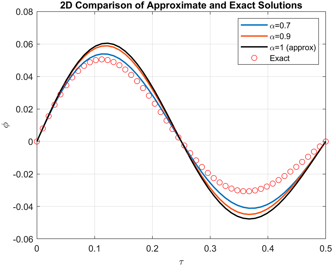
Figure 1. 2D comparison of the approximate (Eq. 69) and exact solution $φ (ξ, x, τ)$ (Eq. 70) for $α = 0.7, 0.9, 1 and ρ = 1.5$ at fixed $ξ and x, varying τ$ .

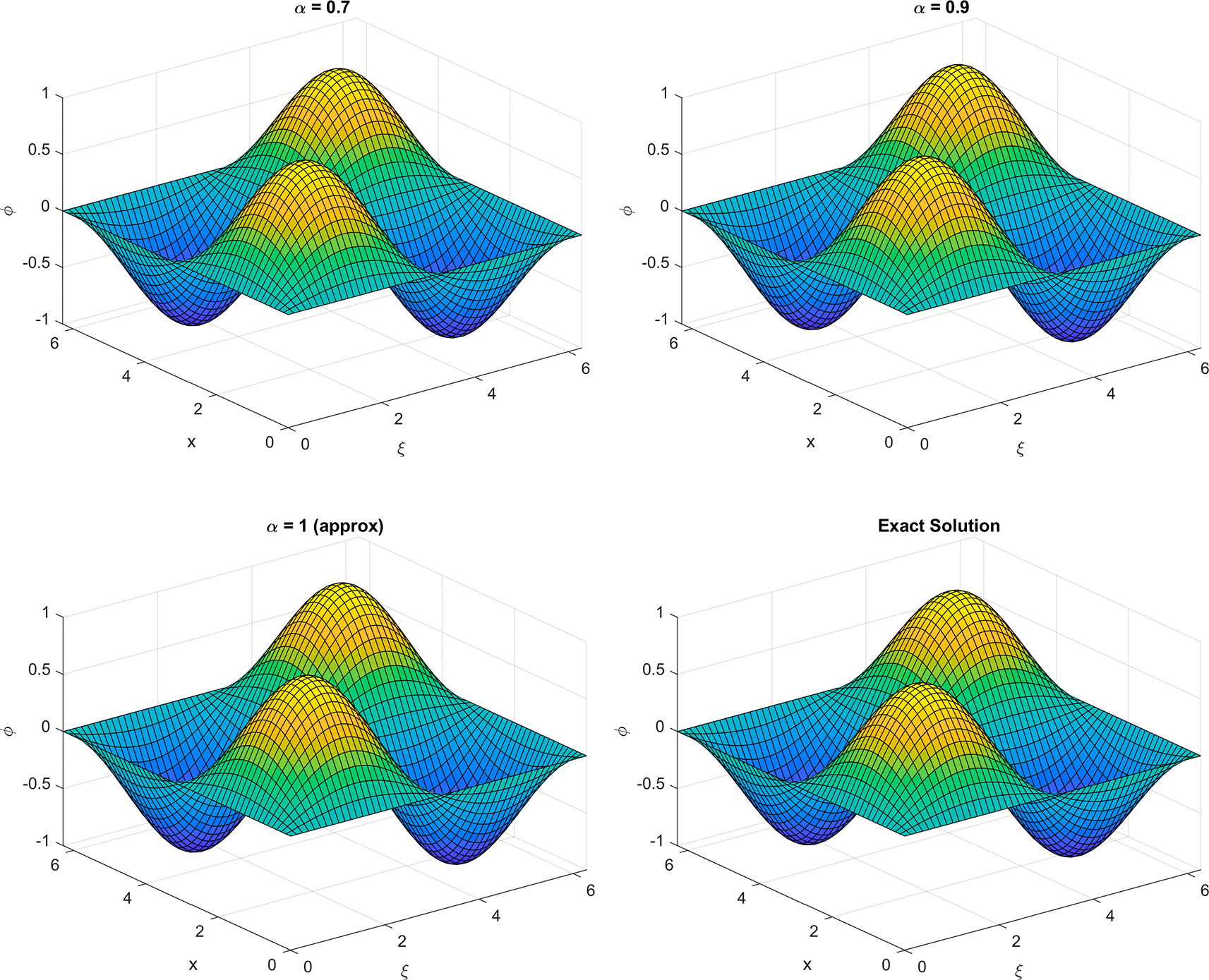
Figure 2. 3D comparison of the approximate (Eq. 69) and exact solution $φ (ξ, x, τ)$ (Eq. 70) for $α = 0.7, 0.9, 1 and ρ = 1.5$ at fixed $ξ and x, varying τ$ .

Let

(75)

φ = \sum_{n = 0}^{\infty} φ_{n},

(76)

φ (ξ, τ) = {}^{ρ}{I_{τ}^{α}} [\sum_{n = 0}^{\infty} {φ_{n}}_{ξξ}] - {}^{ρ}{I_{τ}^{α}} [\sum_{n = 0}^{\infty} φ_{n} \sum_{n = 0}^{\infty} {φ_{n}}_{ξ}] .

(77)

L (φ) = {}^{ρ}{I_{τ}^{α}} [φ_{ξξ}],

(78)

G (φ) = - {}^{ρ}{I_{τ}^{α}} [φ φ_{ξ}] .

The nonlinear terms are

(79)

G_{o} = - {}^{ρ}{I_{τ}^{α}} [φ_{0} \frac{\partial}{\partial ξ} φ_{0}] = - ξ \frac{τ^{ρα}}{ρ^{α} Γ (α + 1)},

(80)

\begin{matrix} G_{1} = - {}^{ρ}{I_{τ}^{α}} [(φ_{0} + φ_{1}) \frac{\partial}{\partial ξ} (φ_{0} + φ_{1})] + {}^{ρ}{I_{τ}^{α}} [φ_{0} \frac{\partial}{\partial ξ} φ_{0}], \\ = ξ (2 \frac{τ^{2 ρα}}{ρ^{2 α} Γ (2 α + 1)} - \frac{τ^{3 ρα}}{ρ^{3 α} {(Γ (α + 1))}^{2} Γ (3 α + 1)}), \\ ⋮ \end{matrix}

The remaining terms can be obtained using the following recurrence relation

(81)

φ_{n + 1} = L (φ_{n}) + G (φ_{n}) .

(82)

φ_{1} = L (φ_{o}) + G (φ_{0}) = - ξ \frac{τ^{ρα}}{ρ^{α} Γ (α + 1)},

(83)

φ_{2} = L (φ_{1}) + G (φ_{1}) = ξ (2 \frac{τ^{2 ρα}}{ρ^{2 α} Γ (2 α + 1)} - \frac{τ^{3 ρα}}{ρ^{3 α} {(Γ (α + 1))}^{2} Γ (3 α + 1)}) .

⋮

As a result, this formulation serves as the approximate solution to the problem,

(84)

φ (ξ, τ) = ξ (1 - \frac{τ^{ρα}}{ρ^{α} Γ (α + 1)} + (2 \frac{τ^{2 ρα}}{ρ^{2 α} Γ (2 α + 1)} - \frac{τ^{3 ρα} Γ (2 α + 1)}{ρ^{3 α} {(Γ (α + 1))}^{2} Γ (3 α + 1)}) + \dots) .

To compare the advantage of the solution, we find the solution of Equation (71) using the Adomian decomposition method with the same operator. We will solve the following approximate solution:

(85)

φ (ξ, τ) = ξ (1 - \frac{τ^{ρα}}{ρ^{α} Γ (α + 1)} + 2 \frac{τ^{2 ρα}}{ρ^{2 α} Γ (2 α + 1)} + \dots) .

Therefore, the exact solution corresponding to Eq. (95) can be expressed as follows:

(86)

φ = \frac{ξ}{1 + τ}, when ρ = α = 1

Table 2, which presents the results using the Daftardar-Jafari Method. Table 3 shows the results using the Adomian decomposition Method. Both tables illustrate the convergence of the approximate solution toward the exact solution for different values of α. By comparing the two tables, we observe that the Daftardar-Jafari Method performs better than the Adomian Method when applied with the same operator.

Table 2. Numerical values of the approximate solution $φ (ξ, τ)$ (Eq. 84) for $α = 0.7, 0.9, 1 and ρ = 1$ at fixed ξ, $and varying τ$ .

$τ$	$φ_{0.7}$	$φ_{0.9}$	$φ_{1}$	$φ_{Exact}$	${Error}_{0.7}$	${Error}_{0.9}$	${Error}_{1}$
0	5	5	5	5	0	0	0
0.05556	4.40524	4.64654	4.73748	4.73684	0.3316	0.0903	0.00063
0.11111	4.15553	4.39042	4.50475	4.5	0.34447	0.10958	0.00475
0.16667	4.00586	4.18785	4.30076	4.28571	0.27985	0.09786	0.01505
0.22222	3.91465	4.0274	4.12444	4.09091	0.17626	0.06351	0.03353
0.27778	3.86255	3.90251	3.97473	3.91304	0.0505	0.01053	0.06168
0.33333	3.83813	3.80856	3.85055	3.75	0.08813	0.05856	0.10055
0.38889	3.83379	3.74195	3.75085	3.6	0.23379	0.14195	0.15085
0.44444	3.84405	3.69969	3.67456	3.46154	0.38252	0.23816	0.21302
0.5	3.86475	3.67924	3.62061	3.33333	0.53142	0.34591	0.28727

Table 3. Numerical values of the approximate solution $φ (ξ, τ)$ (Eq. 85) for $α = 0.7, 0.9, 1 and ρ = 1$ at fixed ξ, $and varying τ$ .

$τ$	$φ_{0.7}$	$φ_{0.9}$	$φ_{1}$	$φ_{Exact}$	${Error}_{0.7}$	${Error}_{0.9}$	${Error}_{1}$
0	5	5	5	5	0	0	0
0.05556	4.41315	4.6472	4.73765	4.73684	0.32369	0.08964	0.00081
0.11111	4.18946	4.39469	4.50617	4.5	0.31054	0.10531	0.00617
0.16667	4.08535	4.20061	4.30556	4.28571	0.20037	0.08511	0.01984
0.22222	4.06009	4.05514	4.1358	4.09091	0.03082	0.03576	0.04489
0.27778	4.09492	3.95319	3.99691	3.91304	0.18187	0.04014	0.08387
0.33333	4.1789	3.89146	3.88889	3.75	0.4289	0.14146	0.13889
0.38889	4.30482	3.86765	3.81173	3.6	0.70482	0.26765	0.21173
0.44444	4.46755	3.87996	3.76543	3.46154	1.00601	0.41842	0.30389
0.5	4.66321	3.927	3.75	3.33333	1.32988	0.59367	0.41667

Figure 3 displays the convergence behavior of the approximate solution as α approaches 1, using the Daftardar-Jafari Method.

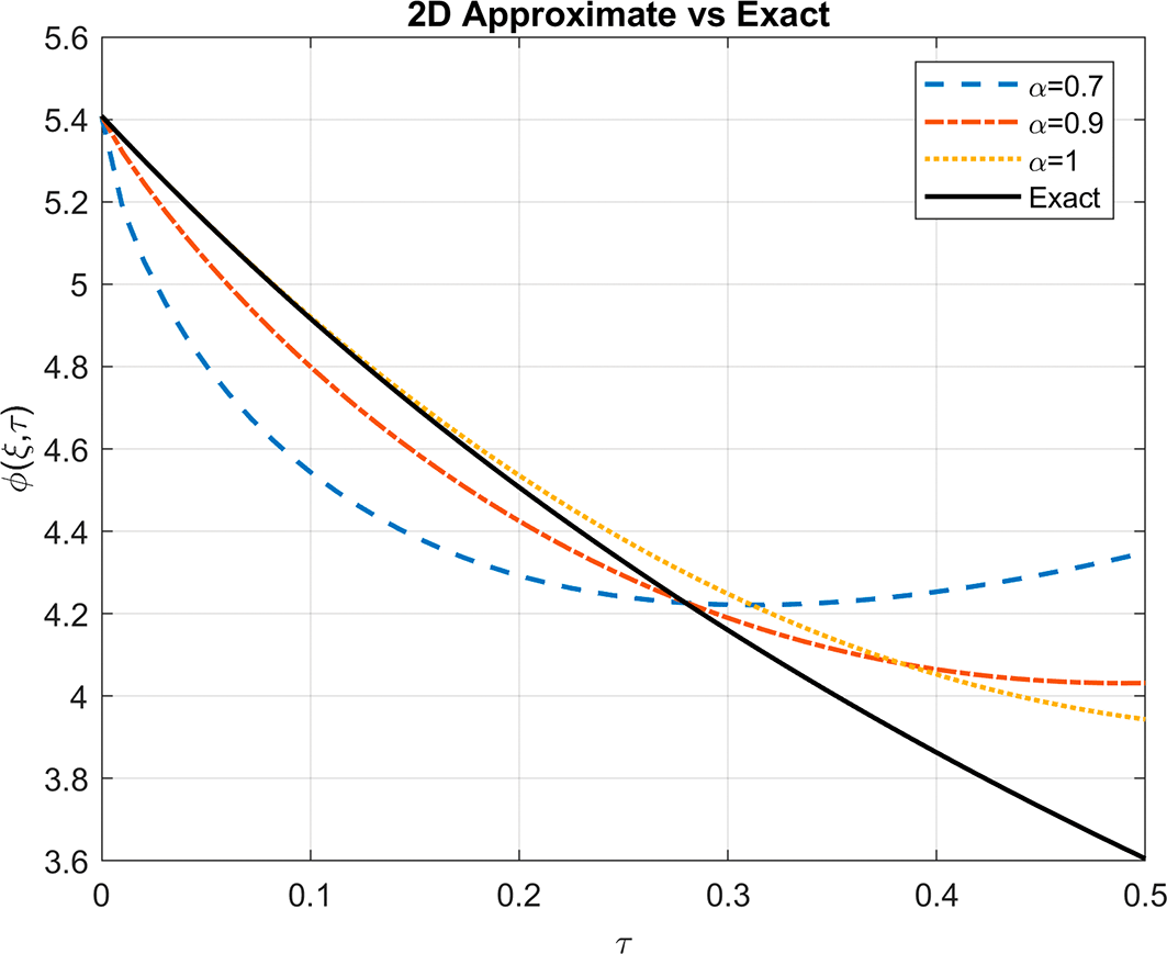
Figure 3. 2D comparison of the approximate (Eq.84) and exact solution $φ (ξ, τ)$ (Eq.86) for $α = 0.7, 0.9, 1 and ρ = 1$ at fixed $ξ, and varying τ$ .

Figure 4 presents a comparison of the convergence between the exact and approximate solutions for the Daftardar-Jafari Method across all tested values of α.

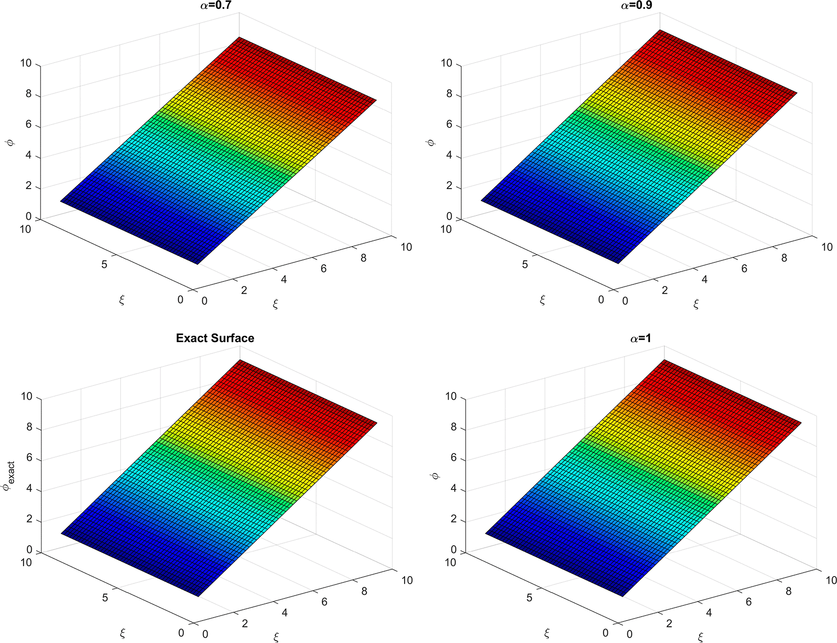
Figure 4. 3D comparison of the approximate and exact solution $φ (ξ, τ)$ (Eq.84) for $α = 0.7, 0.9, 1 and ρ = 1$ at fixed $ξ, and varying τ$ .

5. Discussion

This study presented two illustrative examples to evaluate the performance of the proposed α-generalized Daftardar-Jafari method both analytically and numerically.

In the first example, which involves a linear fractional partial differential equation, the numerical results obtained using the proposed method were comparable to those produced by the Adomian decomposition method. Both approaches yielded identical outcomes. However, from an analytical standpoint, the α-DJM framework offers a simpler and more direct formulation than many existing methods. Furthermore, the approximate solution was observed to converge toward the exact solution as the value of α approached 1. This behavior is clearly demonstrated in Figure 1 and Figure 2.

In contrast, the second example, which involves a nonlinear equation, revealed a distinct advantage of the proposed method. The numerical results obtained using α-DJM were more accurate than those produced by the Adomian method. This is evident from the comparative data presented in Table 2 and Table 3, respectively. Similar to the first example, the convergence of the approximate solution toward the exact solution improved as α approached 1, as illustrated in Figure 3 and Figure 4.

These findings confirm the effectiveness of the α-DJM method, particularly in handling nonlinear fractional models with improved accuracy and convergence behavior.

6. Conclusions

In this work, we introduced a new method for solving both linear and nonlinear fractional partial differential equations. The approach combines the α-generalized fractional differential operator with the Daftardar-Jafari method (DJM). The properties of the α-generalized operator, as presented in this article, demonstrate its generality. In particular cases, it reduces to well-known operators such as Caputo and Hadamard.

We applied the (α-DJM) framework to formulate a detailed solution scheme. This included deriving recurrence relations for both linear and nonlinear equations, and establishing convergence based on Lipschitz conditions through optimization techniques.

Our results show that solving a linear equation using different methods yields similar outcomes. This is clearly illustrated in the first example involving the linear heat equation. The analytical and numerical solutions are identical when substituting the parameters $α = 0.7, 0.9, 1 and ρ = 1.5$ for various values of $τ .$ The second example addresses a nonlinear case involving the Berger equation. Upon solving and comparing with the Adomian decomposition method, we observed noticeable differences in both analytical and numerical results. In this case, we used $α = 0.7, 0.9, 1 and ρ = 1$ for both tables. From the comparative analysis, it is evident that the (α-DJM) method outperforms the Adomian method. It offers better accuracy and consistency.

Overall, the (α-DJM) combines analytical simplicity with numerical efficiency. It provides a unified framework for solving a wide range of fractional models with varying orders.

Future research may extend this framework to incorporate alternative methods and broader comparative studies.

Data citation

Sachit SA, Jassim HK (2025). Dataset for “An Iterative Approach for Solving Fractional Differential Equations Using the α-Generalized Daftardar–Jafari Method”. Zenodo. https://doi.org/10.5281/zenodo.17560489.

Ethics statement

This research does not involve human participants, animal subjects, or sensitive personal data. Therefore, ethical approval was not required.

Data availability statement

The MATLAB scripts used to generate the tables and figures in this article are openly available on Zenodo at: https://doi.org/10.5281/zenodo.17560489.²⁸

Data are available under the terms of the Creative Commons Attribution 4.0 International license (CC-BY 4.0).

Acknowledgments

The authors would like to express their sincere gratitude to the reviewers for their valuable comments and constructive suggestions, which have significantly enhanced the scientific quality of this article. We also extend our heartfelt thanks to the faculty members of the Department of Mathematics at our university for their continuous support and guidance throughout this research.

References

1. Diethelm K, Kiryakova V, Luchko Y, et al.: Trends, Directions for Further Research, and Some Open Problems of Fractional Calculus.2021. Publisher Full Text
2. Jafari H, Jassim HK, Ünlü C, et al.: Laplace Decomposition Method for Solving the Two-Dimensional Diffusion Problem in Fractal Heat Transfer. Fractals. 2024; 32(4): 1–6. Publisher Full Text
3. Jafari H, Jassim HK, Ansari A, et al.: Local Fractional Variational Iteration Transform Method: A Tool For Solving Local Fractional Partial Differential Equations. Fractals. 2024; 32(4): 1–8. Publisher Full Text
4. Jassim H, Ahmad A, Shamaoon CC: An Efficient Hybrid Technique for the Solution of Fractional-Order Partial Differential Equations. Carpathian Math. Publ. 2021; 13: 790–804. Publisher Full Text
5. Cui P, Jassim HK: Local Fractional Sumudu Decomposition Method to Solve Fractal PDEs Arising in Mathematical Physics. Fractals. 2024; 32(4): 1–6. Publisher Full Text
6. Hussein MA, Jassim HK, Jassim AK: An Innovative Iterative Approach to Solving Volterra Integral Equations of Second Kind. Acta Polytechnica. 2024; 64(2): 87–102. Publisher Full Text
7. Jassim HK, Hussein MA: A Novel Formulation of the Fractional Derivative with the Order α≥ 0 and without the Singular Kernel. Mathematics. 2022; 10(21): 4123. Publisher Full Text
8. Khaled Abdeljawad A, et al.: Analysis of a class of fractal hybrid fractional differential equations under Atangana–Baleanu–Caputo derivative. Sci. Rep. 2024; 14. PubMed Abstract | Publisher Full Text | Free Full Text
9. Luchko Y: General fractional integrals and derivatives with the Sonine kernels. arXiv preprint arXiv:2102.04059. Feb. 2021. Publisher Full Text
10. Jafari H, Zayir MY, Jassim HK: Analysis of fractional Navier-Stokes equations. Heat Transfer. 2023; 52(3): 2859–2877. Publisher Full Text
11. Srivastava HM, Baleanu D, Agarwal RP, et al.: Solutions of general fractional-order differential equations by using the spectral Tau method. Fractal Fractional. 2022 Jan.; 6(1): 1–20. art. 7. Publisher Full Text
12. Khalil R, Al Horani M, Yousef A, et al.: A new definition of fractional derivative. J. Comput. Appl. Math. Mar. 2020; 264: 65–70. Publisher Full Text
13. Abdel Latif MS, Abdel Kader AH, Baleanu D: The invariant subspace method for solving nonlinear fractional partial differential equations with generalized fractional derivatives. Adv. Differ. Equ. 2020; 2020(1): 119. Publisher Full Text
14. Sahebi HR, Kazemi M: On the existence of solutions for Hadamard-type fractional integral equations. Bound. Value Probl. 2025; 2025: art. no. 128. Publisher Full Text
15. Taher HG, Ahmad H, Singh J, et al.: solving fractional PDEs by using Daftardar-Jafari method. AIP Conf. Proc. 2022; 2386(060002): 1–10.
16. Balachandran K, Matar M, Annapoorani N, et al.: Hadamard functional fractional integrals and derivatives and fractional differential equations. Filomat. 2024; 38(3): 779–792. Publisher Full Text
17. Guan K, Ou C, Wang Z: Mathematical analysis and a second-order compact scheme for nonlinear Caputo–Hadamard fractional sub-diffusion equations. Mediterr. J. Math. 2024; 21(77): 1–23. Publisher Full Text
18. Sachit SA, Jassim HK: A Modified Iterative Approach Using YJ Transform for Solving Fractional PDEs. Prog. Fract. Differ. Appl. Jan 2015; 1(1): 1–16. Publisher Full Text
19. Jassim HK: A new approach to find approximate solutions of Burger’s and coupled Burger’s equations of fractional order. TWMS J. Appl. Eng. Math. 2021; 11(2): 415–423.
20. Fernandez E, Huilcapi V, Cajo R: The role of fractional calculus in modern optimization: A survey of algorithms, applications, and open challenges. Mathematics. 2023; 13(19): 1–26. Publisher Full Text
21. Guariglia E: Fractional calculus of the Lerch zeta function. Mediterr. J. Math. 2022; 19: 1–18. article no. 109. Publisher Full Text
22. Herrmann R: Fractional Calculus: An Introduction for Physicists. 4th ed.Singapore: World Scientific; 2023. Publisher Full Text
23. Hussain S, Iqbal M, Abbas M: New inequalities for generalized convex functions via fractional integrals. J. Inequal. Appl. 2022; 2022(1): 1–14. article 189. Publisher Full Text
24. Liu W, Liu L: Properties of Hadamard fractional integral and its application. Fractal Fractional. 2022; 6(11): 1–18. article 670. Publisher Full Text
25. Jassim HK, Mohammed MG: Natural homotopy perturbation method for solving nonlinear fractional gas dynamics equations. Int. J. Nonlinear Anal. Appl. 2021; 12(1): 813–821. Publisher Full Text
26. Sweilam NH, Nagy AM, Al-Ajami TM: Numerical solutions of fractional optimal control with Caputo–Katugampola derivative. Adv. Contin. Discret. Models. 2021; 2021: 1–20. article 425. Publisher Full Text
27. Almutairi O, Kılıçman A: New generalized Hermite–Hadamard inequality and related integral inequalities involving Katugampola-type fractional integrals. Symmetry. 2020; 12(4): 1–15. article 568. Publisher Full Text
28. Sachit SA, Jassim HK: Dataset for “An Iterative Approach for Solving Fractional Differential Equations Using the α-Generalized Daftardar–Jafari Method”. Zenodo. 2025. Publisher Full Text

Comments on this article Comments (0)

Version 1

VERSION 1 PUBLISHED 23 Dec 2025

Author details Author details

¹ Mathematics, University of Thi-Qar, An Nasiriyah, Dhi Qar, 64001, Iraq
² Technical Engineering, University of Science and Technology, An Nasiriyah, Dhi Qar, 64001, Iraq

Sahib Abdulkadhim Sachit
Roles: Formal Analysis, Investigation, Methodology, Writing – Original Draft Preparation

Hassan Kamil Jassim
Roles: Investigation, Supervision, Writing – Review & Editing

Competing interests

No competing interests were disclosed.

Grant information

The author(s) declared that no grants were involved in supporting this work.

Article Versions (1)

version 1

Published: 23 Dec 2025, 14:1437

https://doi.org/10.12688/f1000research.172333.1

Copyright

© 2025 Abdulkadhim Sachit S and Kamil Jassim H. This is an open access article distributed under the terms of the Creative Commons Attribution License, which permits unrestricted use, distribution, and reproduction in any medium, provided the original work is properly cited.

Download

Export To

metrics

	Views	Downloads
F1000Research	-	-
PubMed Central Data from PMC are received and updated monthly.	-	-

Citations

0

SEE MORE DETAILS

CITE

how to cite this article

Abdulkadhim Sachit S and Kamil Jassim H. An Iterative Approach for Solving Fractional Differential Equations Using the α-Generalized Daftardar–Jafari Method [version 1; peer review: awaiting peer review]. F1000Research 2025, 14:1437 (https://doi.org/10.12688/f1000research.172333.1)

NOTE: If applicable, it is important to ensure the information in square brackets after the title is included in all citations of this article.

track

receive updates on this article

Track an article to receive email alerts on any updates to this article.

Open Peer Review

Comments on this article Comments (0)

Version 1

VERSION 1 PUBLISHED 23 Dec 2025

Open Peer Review

Reviewer Status

AWAITING PEER REVIEW

Comments on this article

All Comments(0)

Add a comment

Sign up for content alerts

Browse by related subjects

[1] 1. Diethelm K, Kiryakova V, Luchko Y, et al.: Trends, Directions for Further Research, and Some Open Problems of Fractional Calculus.2021. Publisher Full Text

[2] 2. Jafari H, Jassim HK, Ünlü C, et al.: Laplace Decomposition Method for Solving the Two-Dimensional Diffusion Problem in Fractal Heat Transfer. Fractals. 2024; 32(4): 1–6. Publisher Full Text

[3] 3. Jafari H, Jassim HK, Ansari A, et al.: Local Fractional Variational Iteration Transform Method: A Tool For Solving Local Fractional Partial Differential Equations. Fractals. 2024; 32(4): 1–8. Publisher Full Text

[4] 4. Jassim H, Ahmad A, Shamaoon CC: An Efficient Hybrid Technique for the Solution of Fractional-Order Partial Differential Equations. Carpathian Math. Publ. 2021; 13: 790–804. Publisher Full Text

[5] 5. Cui P, Jassim HK: Local Fractional Sumudu Decomposition Method to Solve Fractal PDEs Arising in Mathematical Physics. Fractals. 2024; 32(4): 1–6. Publisher Full Text

[6] 6. Hussein MA, Jassim HK, Jassim AK: An Innovative Iterative Approach to Solving Volterra Integral Equations of Second Kind. Acta Polytechnica. 2024; 64(2): 87–102. Publisher Full Text

[7] 7. Jassim HK, Hussein MA: A Novel Formulation of the Fractional Derivative with the Order α≥ 0 and without the Singular Kernel. Mathematics. 2022; 10(21): 4123. Publisher Full Text

[8] 8. Khaled Abdeljawad A, et al.: Analysis of a class of fractal hybrid fractional differential equations under Atangana–Baleanu–Caputo derivative. Sci. Rep. 2024; 14. PubMed Abstract | Publisher Full Text | Free Full Text

[9] 9. Luchko Y: General fractional integrals and derivatives with the Sonine kernels. arXiv preprint arXiv:2102.04059. Feb. 2021. Publisher Full Text

[10] 10. Jafari H, Zayir MY, Jassim HK: Analysis of fractional Navier-Stokes equations. Heat Transfer. 2023; 52(3): 2859–2877. Publisher Full Text

[11] 11. Srivastava HM, Baleanu D, Agarwal RP, et al.: Solutions of general fractional-order differential equations by using the spectral Tau method. Fractal Fractional. 2022 Jan.; 6(1): 1–20. art. 7. Publisher Full Text

[12] 12. Khalil R, Al Horani M, Yousef A, et al.: A new definition of fractional derivative. J. Comput. Appl. Math. Mar. 2020; 264: 65–70. Publisher Full Text

[13] 13. Abdel Latif MS, Abdel Kader AH, Baleanu D: The invariant subspace method for solving nonlinear fractional partial differential equations with generalized fractional derivatives. Adv. Differ. Equ. 2020; 2020(1): 119. Publisher Full Text

[14] 14. Sahebi HR, Kazemi M: On the existence of solutions for Hadamard-type fractional integral equations. Bound. Value Probl. 2025; 2025: art. no. 128. Publisher Full Text

[15] 15. Taher HG, Ahmad H, Singh J, et al.: solving fractional PDEs by using Daftardar-Jafari method. AIP Conf. Proc. 2022; 2386(060002): 1–10.

[16] 16. Balachandran K, Matar M, Annapoorani N, et al.: Hadamard functional fractional integrals and derivatives and fractional differential equations. Filomat. 2024; 38(3): 779–792. Publisher Full Text

[17] 17. Guan K, Ou C, Wang Z: Mathematical analysis and a second-order compact scheme for nonlinear Caputo–Hadamard fractional sub-diffusion equations. Mediterr. J. Math. 2024; 21(77): 1–23. Publisher Full Text

[18] 18. Sachit SA, Jassim HK: A Modified Iterative Approach Using YJ Transform for Solving Fractional PDEs. Prog. Fract. Differ. Appl. Jan 2015; 1(1): 1–16. Publisher Full Text

[19] 19. Jassim HK: A new approach to find approximate solutions of Burger’s and coupled Burger’s equations of fractional order. TWMS J. Appl. Eng. Math. 2021; 11(2): 415–423.

[20] 20. Fernandez E, Huilcapi V, Cajo R: The role of fractional calculus in modern optimization: A survey of algorithms, applications, and open challenges. Mathematics. 2023; 13(19): 1–26. Publisher Full Text

[21] 21. Guariglia E: Fractional calculus of the Lerch zeta function. Mediterr. J. Math. 2022; 19: 1–18. article no. 109. Publisher Full Text

[22] 22. Herrmann R: Fractional Calculus: An Introduction for Physicists. 4th ed.Singapore: World Scientific; 2023. Publisher Full Text

[23] 23. Hussain S, Iqbal M, Abbas M: New inequalities for generalized convex functions via fractional integrals. J. Inequal. Appl. 2022; 2022(1): 1–14. article 189. Publisher Full Text

[24] 24. Liu W, Liu L: Properties of Hadamard fractional integral and its application. Fractal Fractional. 2022; 6(11): 1–18. article 670. Publisher Full Text

[25] 25. Jassim HK, Mohammed MG: Natural homotopy perturbation method for solving nonlinear fractional gas dynamics equations. Int. J. Nonlinear Anal. Appl. 2021; 12(1): 813–821. Publisher Full Text

[26] 26. Sweilam NH, Nagy AM, Al-Ajami TM: Numerical solutions of fractional optimal control with Caputo–Katugampola derivative. Adv. Contin. Discret. Models. 2021; 2021: 1–20. article 425. Publisher Full Text

[27] 27. Almutairi O, Kılıçman A: New generalized Hermite–Hadamard inequality and related integral inequalities involving Katugampola-type fractional integrals. Symmetry. 2020; 12(4): 1–15. article 568. Publisher Full Text

[28] 28. Sachit SA, Jassim HK: Dataset for “An Iterative Approach for Solving Fractional Differential Equations Using the α-Generalized Daftardar–Jafari Method”. Zenodo. 2025. Publisher Full Text