Introduction
Promotional events are among the most powerful yet short lived mechanisms for driving incremental sales in the consumer packaged goods (CPG) industry. Across categories and retailers, tactics such as temporary price reductions (TPR), feature advertising, in store displays, and combined feature and display campaigns generate measurable sales uplifts followed by predictable decline once the activity ends.1 Although each promotion terminates after a finite period, the sales process often enters a phase of conditional stability. Conditional on the promotion still being active, sales uplift fluctuates within a relatively narrow and stable range.1
This behavior parallels the mathematical construct of a quasi stationary distribution (QSD) in stochastic process theory.2–5 In a QSD framework, the promotion end is treated as an absorbing state, while the active promotional mechanics correspond to transient states through which the system evolves prior to termination. The QSD describes the conditional distribution of sales uplift across these transient states, given that absorption has not yet occurred.3 Formally, if
denotes the promotional state of a product at week
and
is the transition rate matrix governing week to week changes among TPR, Feature, Display, and Feature plus Display, then a distribution
on the non absorbing states satisfies the quasi stationary condition shown in (1). The matrix
represents transition probabilities and
denotes the probability that the promotion remains active at time
:
Differentiating at
yields the eigenvalue form in (2):
where
represents the weekly decay rate or hazard of promotion termination.
6Reinterpreting these stochastic concepts for CPG analytics provides a rigorous statistical foundation for understanding promotion persistence, conditional sales composition, and tactical resilience. The quasi stationary approach captures how promotions evolve prior to termination, linking short term execution dynamics with long term decision intelligence.7
Figure 1 illustrates the overall lifecycle of a promotion from activation to end.
Table 1 summarizes the mapping between stochastic constructs and their CPG promotional equivalents.
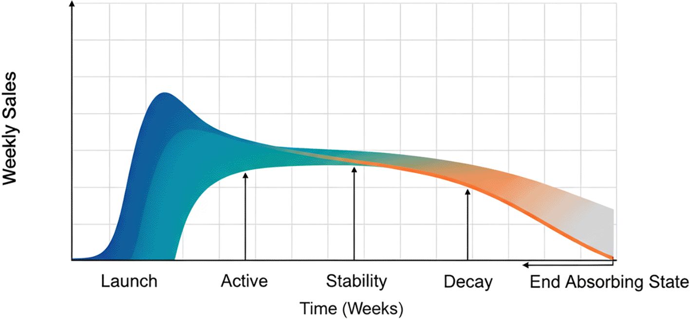
Figure 1. Promotion lifecycle in CPG markets.
The figure illustrates the typical evolution of weekly sales during a promotion, from launch and active phases through stability, decay, and eventual termination, modeled as an absorbing state.
Table 1. Mapping of stochastic constructs to CPG promotional equivalents.
|
Construct | Mathematical meaning | CPG interpretation |
|---|
| Absorbing State | Terminal state the process cannot leave | Promotion end or deactivation |
| Transient States | States visited before absorption | TPR, Feature, Display, Feature+Display |
| Decay Rate
| Eigenvalue governing absorption rate | Weekly probability promotion effectiveness ends |
| Quasi-Stationary Distribution
| Conditional distribution before absorption | Relative share of active promotion mechanics |
| Survival Function
| Probability process remains unabsorbed at time
| Probability a promotion remains active after
weeks |
| Expected Lifetime
| Mean time to absorption | Expected duration of promotional effectiveness |
Related work
The study of quasi-stationary distributions (QSDs) originated in the mid-20th century to describe systems that persist in transient states before eventual absorption. Although developed within branching, diffusion, and Markov processes, the framework naturally extends to promotional dynamics where temporary stability precedes termination.2,6,8–10 The historical progression of quasi-stationary research across foundational decades is summarized in
Figure 2.

Figure 2. Evolution of quasi-stationary distribution research and applications.
The figure summarizes key milestones in the development of quasi-stationary distribution theory, from early branching processes and Markov chain formulations to modern applications in CPG promotion analytics.
Early foundations
Yaglom (1947) analyzed subcritical branching processes and showed that conditional distributions converge to stable forms given non-extinction.2 Bartlett (1955) and Kingman (1963) expanded spectral interpretations linking decay rates to generator eigenvalues.6,8
Markovian formulation
Darroch and Seneta
formalized QSDs for continuous-time Markov chains, proving existence and uniqueness and establishing the canonical relationship
3 Vere-Jones (1969) developed limit theorems and invariance properties,11 while Pakes (1973) connected QSDs to random-walk and catastrophe models.7
Computational advances
From 1991 to 1994, Van Doorn and collaborators introduced numerical methods for quasi-birth-death (QBD) processes, enabling large-scale computation of (
) and bridging stochastic theory with real-world analytics.12,13
A chronological summary of these foundational contributions is provided in
Table 2.
Table 2. Chronological timeline of foundational QSD research (1947-1994).
|
Author(s) |
Year | Primary contribution | Relevance to CPG promotion modeling |
|---|
| Yaglom | 1947 | Introduced quasistationarity in branching processes | Basis for modeling temporary stability such as active promotions. |
| Bartlett | 1955 | Extended QSD to population and diffusion processes | Early integration of stochastic stability in applied systems. |
| Kingman | 1963 | Developed spectral and diffusion interpretations | Provided eigenvalue structure used for decay-rate estimation. |
| Darroch Seneta | 1965-1967 | Formalized QSDs for CTMCs; proved existence and uniqueness | Theoretical basis for matrix driven promotion modeling. |
| Vere-Jones
| 1969 | Established limit theorems for transient Markov systems | Linked conditional long-run behavior to QSD stability. |
| Pakes | 1973 | Connected QSDs to random walks and catastrophe processes | Provided real-world analogs for promotion endings. |
| Kijima Seneta | & | Extended QSDs to renewal and survival models | Bridge to retention and reliability-style marketing models. |
| Van Doorn | 1991–1994 | Numerical QSD methods for QBD processes | Enabled empirical computation of (
) at scale. |
Gap in literature
QSD theory is well established in probability and applied stochastic processes, but there is no prior work applying quasi-stationary analysis to trade promotion effectiveness, conditional sales behavior, or marketing lift persistence. Existing CPG promotion models focus on lift magnitude, elasticity, or carryover effects, whereas QSDs characterize the conditional composition and duration of promotional states before termination. This gap is where our contribution comes in; introducing (
) as interpretable stochastic indicators of promotional persistence and mechanic dominance.
Methods
Theoretical framework
Promotional dynamics in CPG markets can be rigorously modeled as a continuous-time Markov process, where each week corresponds to a transition among distinct promotional states. Let the finite state space be
where “End” denotes the absorbing state representing promotion termination, and all other states form the transient subset
End
.
The process evolves according to a transition-rate matrix
, where
The corresponding transition-probability matrix at time
is
, where each entry
gives the probability of moving from state
to
after
weeks.8 Because every promotion eventually ends, the absorbing state is reached with probability one:
Quasi-stationary condition
A distribution
is quasi-stationary if the conditional distribution over the active states remains constant given that the promotion has not yet ended:
where
is the probability that the promotion remains active at time
.
Differentiating (5) at
yields the key eigenvalue condition:
where
is the decay rate representing the exponential hazard of promotional termination.
3Interpretation for promotions
• The vector
represents the long-run conditional mix of promotion mechanics (TPR, Feature, Display, Feature + Display) given that the promotion is still active.
• The scalar
denotes the weekly hazard rate of promotion termination.
• The survival function gives the probability a promotion remains active after
weeks:
which implies an expected promotional lifespan of
weeks.
Together, these components form a rigorous stochastic structure that captures the balance between temporary stability and inevitable decline within a promotional campaign.2,6
The transition structure among these states is illustrated in
Figure 3. A detailed summary of notation and state definitions is provided in
Table 3.
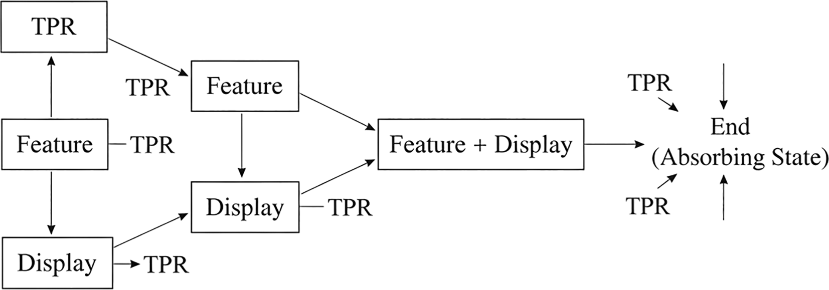
Figure 3. Markov transition structure of promotion states.
The diagram shows allowable transitions between promotional states (TPR, Feature, Display, and Feature + Display) and the absorbing end state, representing promotion termination.
Table 3. State definitions and notation summary.
| Symbol | Definition | Interpretation in CPG context |
|---|
|
| Full state space | All promotion states (TPR, Feature, Display, Feature+Display, End) |
|
| Transient states | Active promotion mechanics still running |
|
| Generator matrix | Week-to-week transitions between promotion states |
|
| Sub-matrix excluding absorbing state | Transitions among active promotion types |
|
| Transition matrix at time
| Probability of moving between states after
weeks |
|
| Quasi-stationary distribution | Conditional share of promotion mechanics while still active |
|
| Absorption rate | Weekly hazard rate of promotion termination |
|
| Survival function | Probability the promotion remains active at week
|
|
| Right eigenvector of
| Expected transitions under QSD conditions |
|
| Time to absorption | Duration until promotion ends |
Promotion-state dynamics
Promotional programs typically cycle through multiple mechanics before termination. A product may move from a TPR to a feature advertisement, subsequently receive a display, or combine both tactics in a feature + display campaign before eventually reverting to base pricing or ending the promotion.1 This evolving structure is captured through a transition network of promotional states with distinct lift patterns.
Let the transient state set be
corresponding to TPR, Feature, Display, and Feature + Display. For active states
, the one-step transition probability is
The self-transition
represents the probability that a promotion remains in the same configuration for an additional week. Empirically estimating these probabilities across weeks yields the transition sub-matrix
that governs pretermination behavior.3
Interpretation of transitions
• TPR → Feature/Display: escalation from price-only tactics toward awareness-building mechanisms.
• Feature + Display → End: termination following a high-intensity promotional phase.
• Self-loops
: persistence of the same promotional mode (e.g., consecutive display weeks).
These transitions shape both the persistence probability and the conditional composition vector
in the quasi-stationary regime.
Empirical transition example
The empirical transition matrix is estimated as the proportion of weeks in which a promotion moved from state
to
in the simulated 104-week dataset:
The resulting matrix
is row-sub-stochastic: each row sums to less than one, with the remainder representing transition to the absorbing “End” state.6 These probabilities feed directly into the eigenvalue decomposition used to derive (
), as discussed in Section.
A visual representation of week-to-week transitions among promotional mechanics is shown in
Figure 4. An illustrative set of weekly transition probabilities is provided in
Table 4.
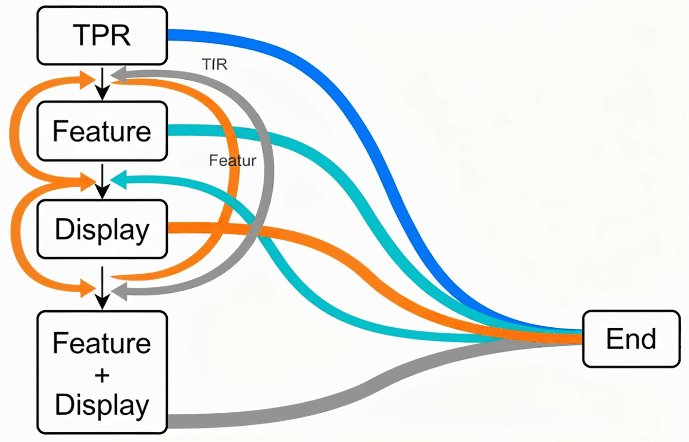
Figure 4. Week-to-week transition flow of promotion states.
The figure illustrates the probabilistic transitions between promotion mechanics (TPR, Feature, Display, and Feature + Display) and convergence to the absorbing end state over time.
Table 4. Example weekly transition probabilities (Retailer-UPC level).
| From
To | TPR | Feature | Display | F+D |
End |
|---|
| TPR | 0.55 | 0.10 | 0.10 | 0.10 | 0.15 |
| Feature | 0.15 | 0.40 | 0.10 | 0.15 | 0.20 |
| Display | 0.10 | 0.15 | 0.45 | 0.10 | 0.20 |
| Feature
Display | 0.10 | 0.10 | 0.20 | 0.50 | 0.10 |
Analytical estimation framework
The quasi-stationary framework quantifies promotional persistence and the conditional composition of active promotion types. Operationally, it estimates how long a promotion remains effective before termination and the distribution of promotion mechanics during its active life.1
Let
denote the sub-generator among transient states (excluding the absorbing End state). If the transition matrix among active states is written as
, then the taboo survival function for a promotion starting in state
is:
The exponential decay implies that the probability of a promotion still being active declines at rate
, the dominant eigenvalue of
3 The corresponding left eigenvector
defines the quasi-stationary distribution:
The expected duration of promotional effectiveness follows:
As shown earlier in Figure 3, this structure captures how promotions transition among mechanics before eventual termination.
Eigenvalue and spectral characterization
Let
denote the eigenvalues of
, ordered such that:
The principal eigenvalue
determines the slowest decaying component of the process and governs long-term survival behavior.3,5,6 The decay rate may be characterized through the functional determinant:
which identifies the dominant root associated with promotional decay.
7Computational estimation
The empirical estimation procedure proceeds as follows:
1. Construct the empirical
from observed week-to-week transitions among active promotions.
2. Compute eigenvalues and corresponding left eigenvectors of
.
3. Identify
as the principal decay rate (smallest magnitude real eigenvalue).
4. Normalize the associated left eigenvector to obtain the quasi-stationary distribution
.
This procedure allows scalable estimation at the UPC, brand, or category level, enabling continuous monitoring of promotional persistence patterns.12
The corresponding eigenvalue spectrum that guides the identification of the dominant decay rate
is shown in
Figure 5.
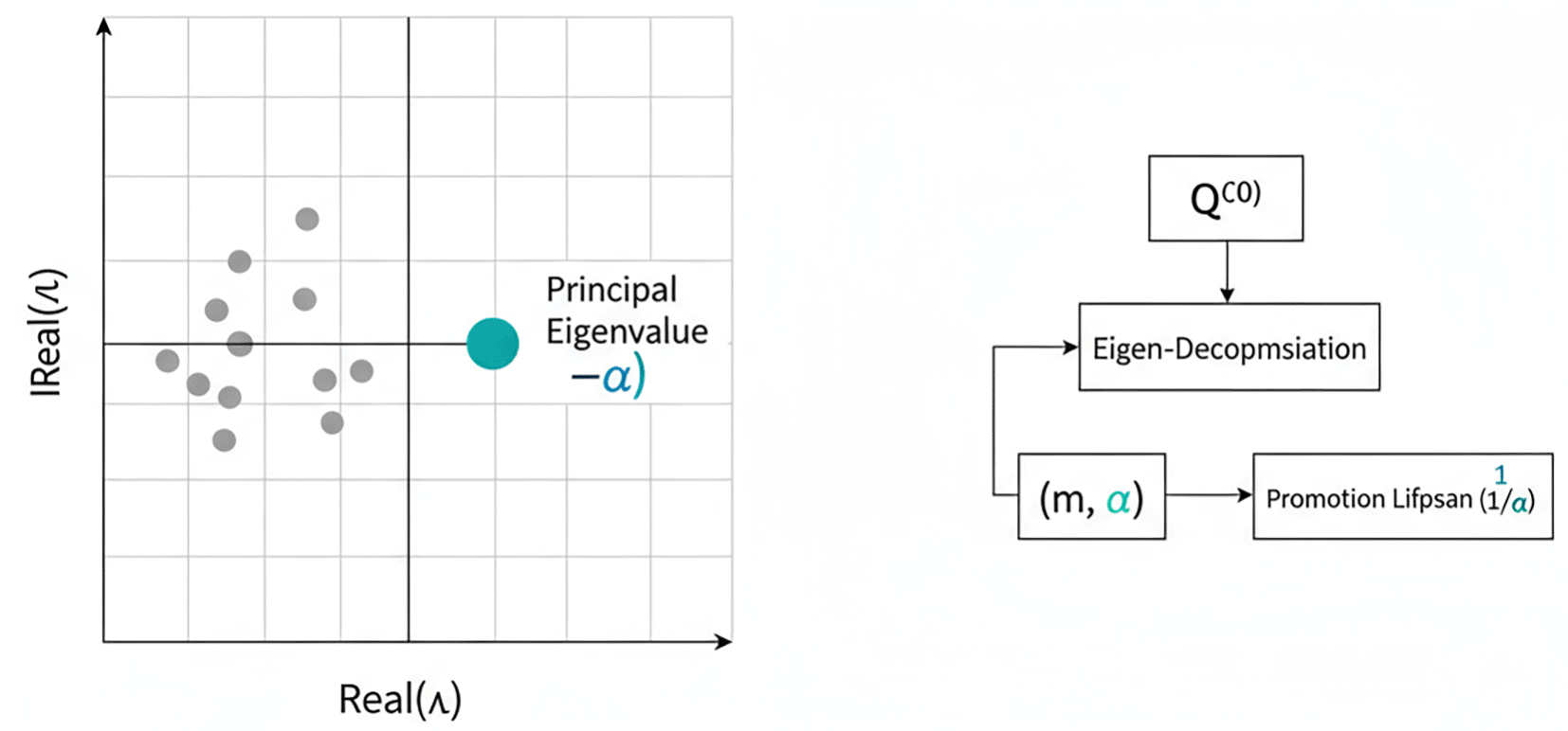
Figure 5. Eigenvalue spectrum and analytical estimation framework.
The figure shows the eigenvalue spectrum of the transition matrix, highlighting the principal eigenvalue used to estimate the dominant decay rate, along with the analytical workflow for deriving promotion lifespan and quasi-stationary state composition.
As summarized in
Table 5, the decay rate and QSD composition vary across categories, reflecting differences in promotional strategy and consumer response.
Table 5. Summary of estimated quasi-stationary parameters across categories (illustrative).
| Category |
|
(wks) |
Dominant
|
|---|
| Beverages | 0.12 | 8.33 | Feature + Display |
| Dairy | 0.14 | 7.14 | Feature |
| Household | 0.23 | 4.35 | TPR |
Empirical applications
We estimate (
) using simulated multi-category promotional data. Each category reflects distinct dynamics in promotional persistence, decay rate, and conditional state composition.1
Category-level parameter estimation
Weekly UPC-retailer promotional histories are used to construct the empirical transition sub-generator
. Eigenvalue decomposition produces the decay rate
and the quasi-stationary composition vector
. The probability that a promotion remains active after
weeks is given by the survival function in (14):
The associated expected promotional lifespan is
3
Interpretation across categories
Feature + Display typically exhibits the lowest decay rate
(longer promotional persistence), TPR is moderate, and Display-only often yields higher
values (faster decay). Categories such as beverages and dairy show long-lived promotional cycles, while certain household categories exhibit more rapid decline.12
Managerial insights
The decay rate
supports decisions on optimal promotion duration. Campaigns with small
benefit from extended runs, whereas campaigns with large
are best rotated or terminated quickly. The QSD vector
provides tactical allocation weights for funding promotion types that sustain conditional lift.
The decay profile and corresponding survival function are illustrated in
Figure 6.
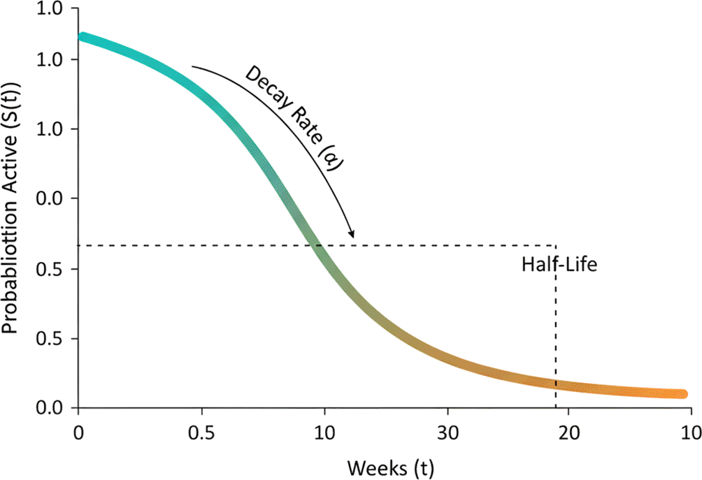
Figure 6. Promotion decay curve and survival function.
The figure shows the exponential survival function
, illustrating the probability that a promotion remains active over time and the associated half-life determined by the decay rate
.
Table 6 summarizes estimated parameters across representative categories.
Table 6. Summary of estimated quasi-stationary parameters across CPG categories (illustrative).
| CategoryDom. Type | Decay
| Life
|
Conditional Mix
|
|---|
| BeveragesF+D | 0.14 | 7.1 | (0.18, 0.22, 0.25, 0.35) |
| Snacks | 0.22 | 4.5 | (0.30, 0.40, 0.20, 0.10) |
| Personal TPR Care | 0.18 | 5.6 | (0.35, 0.25, 0.20, 0.20) |
| HouseholĐisplay | 0.26 | 3.8 | (0.20, 0.15, 0.45, 0.20) |
| Dairy | 0.12 | 8.3 | (0.15, 0.25, 0.25, 0.35) |
Experimental validation
We construct a 104-week simulated UPC-retailer dataset with weekly transitions among TPR, Feature, Display, Feature + Display, and the absorbing End state. This controlled environment enables validation of the quasi-stationary estimation of
.
Dataset and simulation structure
Each weekly observation includes promotional state and sales. Transitions follow a predefined matrix ensuring eventual absorption, emulating real-world cycles in which lift diminishes after repeated exposure.1 A subset of the simulated 104-week promotional dataset is shown in
Table 7.
Table 7. Sample data excerpt from 104-week simulation (promo_data.csv).
| Week | Promo state |
Sales (Units) |
|---|
| 1 | Feature | 298.3 |
| 2 | Display | 274.6 |
| 3 | Feature + Display | 369.9 |
| 4 | Feature + Display | 392.5 |
| 5 | Feature | 312.4 |
| 6 | Display | 281.7 |
| 7 | TPR | 265.8 |
| 8 | TPR | 254.2 |
| 9 | Feature + Display | 401.3 |
| 10 | End | 190.7 |
Estimating transition matrix and parameters
Let
denote transitions from state
to
. The empirical transition probabilities are estimated as:
The quasi-stationary parameters follow from the eigen-decomposition:
Results
Table 8 shows strong persistence in Feature + Display (0.50) and TPR (0.56), indicating durable campaigns. Feature and Display rotate more frequently through awareness-driven transitions (0.16-0.22).
Table 8. Estimated transition matrix
from 104-week simulated data.
| From → To | TPR | Feature | Display |
F+D |
|---|
| TPR | 0.56 | 0.12 | 0.14 | 0.18 |
| Feature | 0.18 | 0.42 | 0.22 | 0.18 |
| Display | 0.22 | 0.16 | 0.43 | 0.19 |
| Feature + Display | 0.15 | 0.16 | 0.19 | 0.50 |
The resulting quasi-stationary composition is:
The resulting quasi-stationary composition vector is summarized in
Table 9.
Table 9. Quasi-stationary composition
derived from
Table 8.
| State |
m
i |
|---|
| TPR | 0.293 |
| Feature | 0.200 |
| Display | 0.239 |
| Feature + Display | 0.268 |
Survival function and diagnostics
The survival curve follows:
The corresponding empirical survival curve and its fitted exponential decay are shown in
Figure 7.
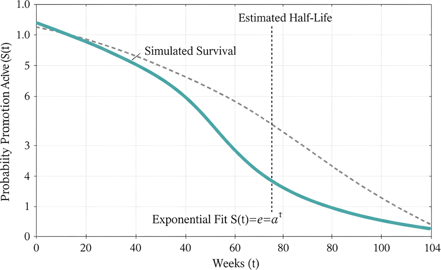
Figure 7. Promotion survival curve with empirical and fitted decay.
The figure compares the empirical promotion survival trajectory with the fitted exponential decay function
, highlighting the estimated promotion half-life.
The transition intensities across active promotion mechanics are visualized in the heatmap shown in
Figure 8.
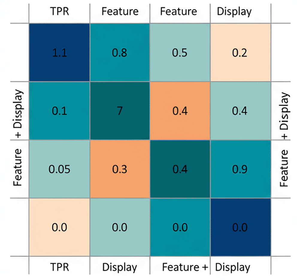
Figure 8. Transition probability heatmap among active promotion states.
The heatmap shows estimated transition intensities between promotion mechanics (TPR, Feature, Display, and Feature + Display), illustrating the relative likelihood of movement across states during active promotions.
Validation
Empirical-theoretical alignment validates QSD applicability for promotional persistence.12 Longevity depends not only on duration but also on tactical transitions, complementing machine-learning uplift and BSTS models used in planning dashboards.
Managerial implications
Translating (
) into operational decisions enables optimization of promotion duration, mechanic rotation, and return on investment (ROI).1 A visual summary of these decision zones, based on the decay rate
, is shown in
Figure 9.
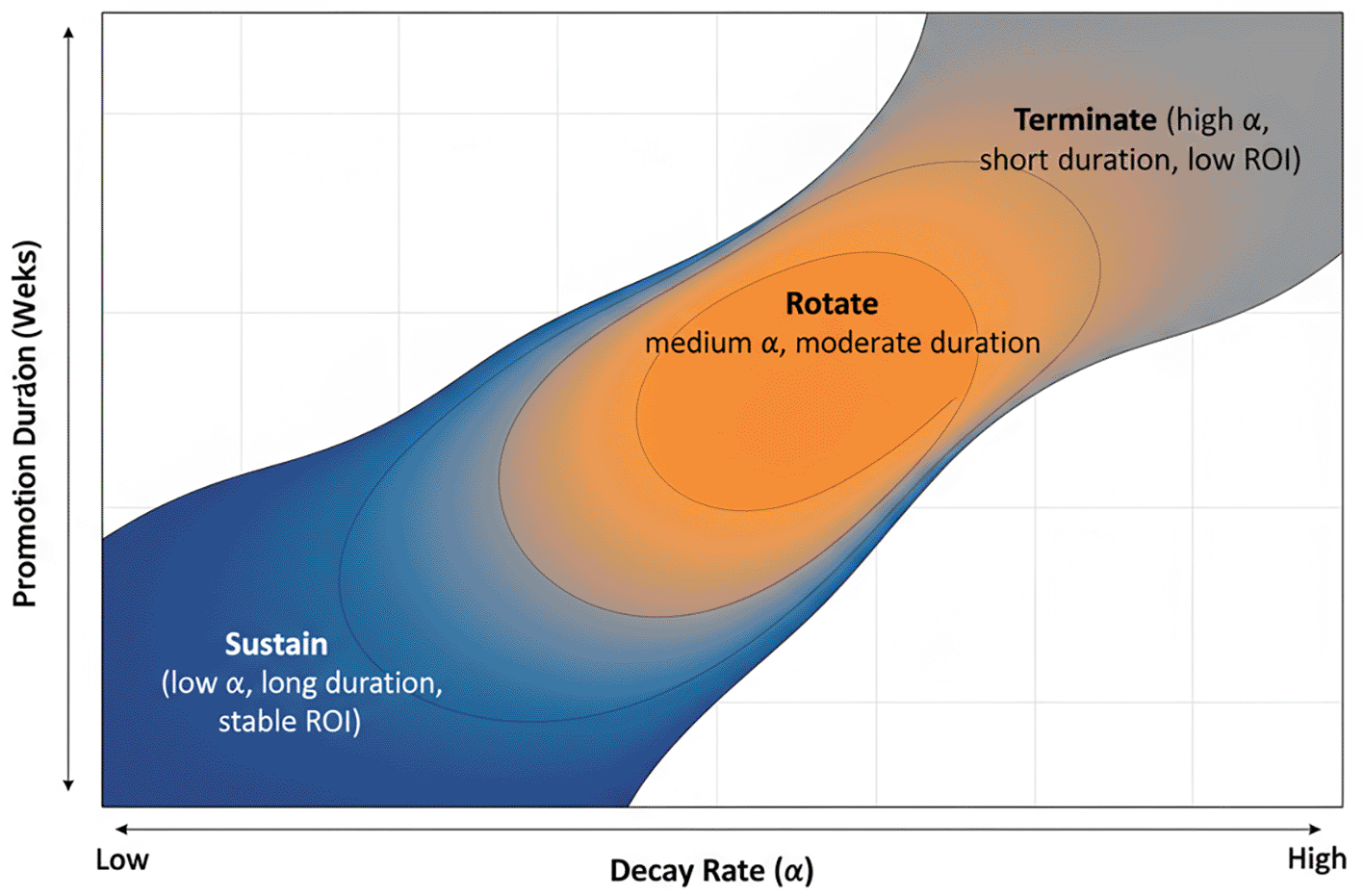
Figure 9. Decision matrix for promotion duration versus decay rate.
The figure maps promotion duration against the estimated decay rate
, illustrating decision regions for sustaining, rotating, or terminating promotions based on expected lifespan and ROI considerations.
Strategic use of decay rate
A lower decay rate indicates longer promotional persistence.
•
between 0.10 and 0.14: long-lived promotions.
•
between 0.15 and 0.20: moderate stability; rotate mechanics.
•
above 0.25: rapid decay; redesign or terminate.7
Even small increases in
significantly reduce the expected lifespan
.
Tactical insights from
The quasi-stationary composition
indicates which tactic dominates conditional effectiveness:
• High
: display-sensitive categories-invest in co-located displays.
• High
: price-driven elasticity dominates.
• Use
to prioritize sequencing and budget allocation.
Decision matrix and dashboards
Decision zones include Sustain (low
), Rotate (moderate), and Terminate (high).12 These rules can be integrated into enterprise dashboards for stop/continue signals (based on
), expected duration (
), and mechanic mix (
).
A detailed summary of decision rules by decay rate, expected lifespan, and ROI implications is provided in
Table 10.
Table 10. Managerial insights: promotion duration, ROI, and α sensitivity.
| Decay rate
| Life (
) | Action | Strategic insight |
ROI trend |
|---|
| 0.100.14 | 7-10 weeks | Sustain | Strong conditional stability; maintain plan | High |
| 0.150.20 | 5-6 weeks | Rotate | Moderate persistence; rotate between tactics | Moderate |
| 0.210.28 | 3-4 weeks | | Terminate Rapid decay; short-term lift only | Declining |
| > 0.28 | < 3 weeks | Redesign | High fatigue; requires new strategy | Low |
Integration into marketing dashboards
Quasi-stationary metrics integrate naturally into enterprise analytics platforms (e.g., Circana’s Demand Forecaster or Promo Effectiveness Dashboard). Key indicators include:
•
: hazard of promotional fatigue (stop-continue signal)
•
: expected effective weeks of lift
•
: conditional probability of each promotion tactic
Aligning these indicators with profitability and media effectiveness enables stochastic decision optimization: a discipline that quantifies persistence, lift decay, and mechanic efficiency in a unified framework.3,14
Conclusion
The eigenvalue relation
provides a unified structure for describing conditional promotional composition, persistence, and decay. It supports descriptive analysis (state evolution), predictive modeling (survival
), and prescriptive guidance (optimal duration and rotation). A smaller
signifies more durable promotions, while a larger
signals rapid decay, guiding tactical allocation and execution.3,12
Future extensions may incorporate multi-retailer heterogeneity in
, competitive interactions, and transition-probability learning from large-scale scanner and loyalty datasets.
Future work
Future work may extend the proposed quasi-stationary promotion framework to empirical retailer–UPC scanner datasets to validate performance under real-world noise, seasonality, and execution constraints. Extensions to transition matrices that depend on time could capture calendar effects, promotion fatigue, and changing consumer responsiveness over time. The framework may also be generalized to competitive settings, where multiple brands interact and promotion termination depends on cross-brand dynamics. Finally, integrating quasi-stationary metrics with machine learning–based uplift and forecasting models represents a promising direction for embedding stochastic persistence measures into operational promotion planning systems.
Ethics and consent
No human subjects, private data, or biological specimens were involved.
Data availability
All data used in this study are simulated and fully reproducible and are openly available.
The simulated promotion dataset supporting the findings of this study is available in the GitHub repository and includes a 104-week retailer–UPC–level promotion history generated using the proposed quasi-stationary framework:
The dataset does not contain any proprietary, confidential, or third-party commercial data. All data are author-generated and intended solely for methodological demonstration and validation.
An archived version of the dataset is available via Zenodo:
Gunasekaran, V. (2025). Quasi-Stationary Dynamics of CPG Promotions – Simulated Data and Code. Zenodo - https://doi.org/10.5281/zenodo.17925573.15
Data are available under the terms of the Creative Commons Attribution 4.0 International license (CC-BY 4.0).
Software availability
Source code available from: https://github.com/vinoalles/Quasi
Archived source code available from: https://doi.org/10.5281/zenodo.17925573
License: MIT License (OSI-approved)
Reporting guidelines
This study does not involve clinical trials, human participants, animals, or qualitative research, and therefore does not require CONSORT, STROBE, ARRIVE, or COREQ/SRQR reporting checklists. The article follows the general reproducibility and transparency standards recommended by F1000Research for computational research.
Acknowledgements
The authors thank contributors to open-source recommender-system libraries.
References
- 1.
Gupta S, Cooper LG:
The discounting of promotional effects in consumer markets.
J. Mark. Res.
1992; 29(2): 223–237.
- 2.
Yaglom AM:
Certain limit theorems of the theory of branching stochastic processes.
Dokl. Akad. Nauk SSSR.
1947; 56: 795–798.
- 3.
Darroch JN, Seneta E:
On quasi-stationary distributions in absorbing continuous-time finite markov chains.
J. Appl. Probab.
1965; 2(1): 88–100. Publisher Full Text
- 4.
Philip K:
Pollett. Quasi-stationary distributions.
Probab. Surv.
2015; 12: 1–35.
- 5.
Collet P, Martínez S, Martín JS:
Quasi-Stationary Distributions: Markov Chains, Diffusions and Dynamical Systems.
Berlin:
Springer;
2013.
- 6.
Kingman JFC:
On the algebra of queues and the spectral theory of markov chains.
J. Appl. Probab.
1963; 1(2): 252–282.
- 7.
Pakes AG:
Some limit theorems for markov chains with applications to population theory.
Adv. Appl. Probab.
1973; 5: 68–95.
- 8.
Bartlett MS:
An Introduction to Stochastic Processes with Special Reference to Methods and Applications.
Cambridge:
Cambridge University Press;
1955.
- 9.
Pollett PK:
Quasi-stationary distributions: A bibliography.
Electron. J. Probab.
2001; 6: 1–33.
- 10.
Van Doorn EA:
Quasi-stationary distributions and convergence to quasi-stationarity.
J. Appl. Probab.
2013; 50(4): 1038–1056.
- 11.
Vere-Jones D:
Some limit theorems for evanescent processes.
J. Appl. Probab.
1969; 11(2): 67–78. Publisher Full Text
- 12.
Van Doorn EA, Schrijner P:
Quasi-stationary distributions for discrete-time markov chains.
Adv. Appl. Probab.
1994; 26(3): 706–720.
- 13.
Méléard S, Villemonais D:
Quasi-stationary distributions and population processes.
Probab. Surv.
2012; 9: 340–410. Publisher Full Text
- 14.
Puterman ML:
Markov Decision Processes: Discrete Stochastic Dynamic Programming.
New York:
John Wiley & Sons;
1994.
- 15.
Gunasekaran V:
Quasi-Stationary Dynamics of CPG Promotions: Simulated Data and Code.
Zenodo.
2025. Publisher Full Text


Comments on this article Comments (0)