Assessing psychogenic health risks through the days between death and birth in the individual annual cycle

Introduction

The term “birthday effect” has been used to designate increased mortality on or around birthdays. Based on a wide range of data and analysis methods, both supportive and contradictory results from different populations and subgroups have been published since the late 1970s, including findings on reduced birthday-related mortality. Three often cited large population-based studies have reported birthday and post-birthday mortality increases. Alderson (1975), in national mortality records from England and Wales (1972), found an increase in deaths on the birthday month and over the months following. Phillips et al. (1992), in California death registration data (1978-1990), observed increased mortality primarily in the week following birthdays, with the effect being stronger in women than men. Ajdacic-Gross et al. (2012), in Swiss mortality records (1969-2008), found elevated mortality on the birthday itself and shortly after, especially among women. Among the three studies, the mortality increases on birthday ranged from one to almost 14 percent.

Focusing on deaths from causes other than suicide, several studies, in addition to Alderson (1975) and Ajdacic-Gross et al. (2012), have found increased mortality on the birthday itself. Grigsby (1985; US National Mortality Survey, 1966-1968) found more deaths, particularly of cardiovascular causes, in the month of the birthday. Vaiserman et al. (2003; Ukrainian mortality records, 1990-2000) reported mortality increases of about 44 percent in men and 36 percent in women on the day of birth. Bovet et al. (1997; Swiss mortality records, 1969-1992) reported increases of 15 percent in men and 19 percent in women compared to expected levels on the day of birth. Peña (2015; US mortality records, 1998-2011) reported an excess death rate of 6.7 percent on birthdays.

Post-birthday mortality increases, which might indicate postponement effects, have been observed in other studies besides those of Alderson (1975), Phillips et al. (1992), and Ajdacic-Gross et al. (2012). Byers et al. (1991; Ohio mortality records, 1979-1981) reported an excess in deaths of about five percent in the month following compared to the month preceding the birthday. Comparing deaths occurring during the quarters before and after the birthday, Kunz and Summers (1980; US data from various sources) found that almost half of all deaths occurred in the quarter after the birthday, both for natural and non-natural causes. The same pattern of results was reported by Shimizu and Pelham (2008; based on more than 30 million US death records), with people more likely to die just after rather than just before their birthday. Further pre-birthday effects have been published by Phillips et al. (1992), who found a dip in deaths before birthdays in women, and by Grigsby (1985), who found a dip in cardiovascular deaths in the month before the birthday. Increased levels of fatal accidents have been reported before (as well as on) birthdays (e.g., Greiner & Pokorny, 1989; Ajdacic-Gross et al., 2012; Matsubayashi & Ueda, 2016).

Conversely, Greiner and Pokorny (1989; US cohort of male veterans with mental disorders, 1972-1978) as well as Brenn and Ytterstad (2003; Norwegian mortality records, 1991-1995) did not find birthday effects. Studies focusing on special populations and methods have provided limited insights into the birthday effect. Stumpfe (1983), based on collecting newspaper death notices (Cologne, Germany, 1979-1980) and Angermeyer et al. (1987), examining celebrities, reported no birthday effects. Other such studies have found birthday effects: Phillips and Feldman (1973), investigating biographical information on famous persons; Abel and Kruger (2009), investigating baseball players (up to 2004); Kelly and Kelleher (2018), collecting dates of birth and death of famous individuals on the internet. These studies suffer from combinations of low statistical power, potential selection bias due to unconventional sampling methods, and limited generalizability.

Regarding specific causes of death, Brown and Knapp (1995; New York and Ohio cancer registries, 1989) reported no differences in mortality levels in cancer patients near birthdays compared to more remote periods. Likewise, Young and Hade (2004; Ohio cancer registry data, 1989-2000) as well as Medenwald and Kuss (2014; German cancer registry data, 1995-2009) found no evidence of altered mortality among cancer patients around their birthdays. Research on cancer has therefore thus far provided quite consistent findings of no effect. Interestingly, cancer mortality also does not seem to exhibit the seasonality seen in many other causes of death (Young & Hade, 2004).

The results on suicide are mixed. Several studies found increased suicide risks on as well as before and after birthdays, often with stronger effects observed in men than in women. Barraclough and Shepherd (1976; UK sample of 247 suicides), Kunz (1978; German suicide data), Zonda et al. (2010; Hungarian suicide data, 1970-2002), Stickley et al. (2016; Tokio suicide registration, 2001-2010), Matsubayashi and Ueda (2016; Japanese mortality records, 1974-2014) and Matsubayashi et al. (2019; Japanese mortality records, 1974-2014), all reported increased suicide mortality risks. For instance, Zonda et al. (2010) and Stickley et al. (2016) found that the increase in suicides around birthdays ranged from about ten to 45 percent, indicating a robust birthday effect. In contrast, several other studies did not find an association between suicides and birthday periods, including Lester (1986, 1997, Medical Examiner of Philadelphia, (212 suicides of 1982), and sample of 201 famous suicides with complete dates of birth and death, respectively), Wasserman and Stack (1994; Ohio suicide records, 1989-1991), Panser et al. (1995; Olmsted county, Minnesota, suicide data), Chuang and Huang (1996; Taiwan suicide registration), Jessen and Jensen (1999; Danish suicide register, 1970-1994), Reulbach et al. (2007; German mortality records, 1998-2003), Williams et al. (2011; UK mortality records), and Deisenhammer et al. (2018; Austrian suicide records, 1994-2014).

The heterogeneity in published results, methods, and reporting is so pronounced that trying a meta-analysis has all the makings of a non-starter. Rather, addressing the methodological shortcomings of existing research seems to be more promising. Many studies are small and do not cover whole populations, fail to adjust for the well-established effects of season (cf. Marti-Soler et al., 2014) and day of the week (cf. Trudeau, 1997; Brenn & Ytterstad, 2003), do not address potential systematic errors such as age-related mortality gradients (Roger, 1977) and heaping (Abel & Kruger, 2006), and neglect to stratify findings by demographic and diagnostic groups. The time resolution of the analysis varies greatly, from days to weeks to months to quarters, and many publications also do not provide precision statistics alongside point estimates, and often have inadequately described methods and give insufficient descriptive results. Additionally, the use of non-comparable statistics, such as counts instead of rates, hinders assessing results across studies. While this is a bleak outlook after half a century of research on the matter, it highlights the opportunity to address the identified shortcomings. Consequently, the present study aims to overcome these issues and maximize methodological rigor in exploring potential birthday effects.

With the evidence heterogeneous and the validity of the underlying data as well as their analyses questionable, not only is the magnitude, distribution, and nature of the phenomenon currently unclear, but its very existence is uncertain. This raises the fundamental question as to why one should continue investigating a phenomenon that, if it exists at all, has at best a minimal impact on mortality, largely lacks any discernible potential for prevention, and is fraught with methodological challenges. The answer lies in its unique opportunity to investigate the role of psychogenic factors in death and, by extension, in health more generally.

Whereas ultimately death always entails the unsustainable loss of the structural or functional form of the body or some of its parts, its less proximate causes fall into three rather disparate and broad categories, namely external (often regarded to include both environmental and social factors), somatic, and psychogenic factors. As people keep on living, repeated and accumulating exposures to external, bodily, and subjective-behavioral factors combine and accumulate in numerous ways to eventually manifest as specific diseases, conditions, or injuries that ultimately lead to death. These underlying states are categorized into major groups, most famously by the International Classification of Diseases. While environmental, social, and (increasingly) biological risk factors lend themselves to objective measurement and epidemiological assessment, things are more complicate when it comes to psychological ones. For some health-related behaviors (like the use of toxic substances or the lack of physical activity) and their consequences (like obesity), and to a lesser extend for others (like nutrition), good progress has been made over the last few decades on quantifying their relevance. Estimates of their combined impact on total mortality, in particular in Western countries, of more than 50 percent are not uncommon (e.g., Knoops et al., 2004). In contrast, investigating non-behavioral psychogenic factors is considerably more challenging. Aside of fundamental conceptual challenges (mind-body problem) and problems of objective measurement, there is the notorious issue of psychological variables (e.g., emotional states) always being under the influence of biological factors which in turn are, naturally, linked to health. As a result, any empirical association between non-behavioral psychogenic factors on the one hand, and any kind of health outcome (including death) on the other, is prone to – typically unmeasured – confounding by biological variables. This is the fundamental methodological problem of psychosomatic research.

A route to circumvent the threats of unmeasured confounding has been the use of instrumental variables (cf. Angrist et al., 1996), a common challenge being to find a valid instrument. In the current context, the instrument would have to stand in for non-behavioral psychological measurements. The advantage of having a valid instrumental variable would be, if certain general conditions hold, that associations between the instrument and the outcome (death) could not be confounded by biological variables. These conditions, often referred to as relevance, exclusion restriction (birthdays conditionally independent of outcomes given psychological factors), and independence (birthdays uncorrelated with any cause of the outcome), would in the present context come down to the instrument causally affecting death, but only through its impact on psychological variables, and itself not being caused by a factor that also causes death. In psychosomatic research, it has long been noted (even if not always in so many words) that life events can be instrumental variables. However, life events present technical challenges, such as lack of uniform definitions or availability in civil registration databases (e.g., changing working conditions, vacations, or relationships). Others, with clear definitions and general applicability, are compromised by closely associated social events (e.g., New Year's Eve or national holidays), making it difficult to separate individual from group effects. In contrast, birthdays are reliably documented in public records and are independent of general social events or the birthdays of others which, other than with public anniversaries, warrants stable unit effects through non-interference and absence of individual- and group-level spillover.

In spite of these advantageous properties, there are four main reasons why birthday – or more specifically, the death-to-birth day interval (DB difference) – is not a carefree variable. First, its validity as an indicator of psychogenic mortality effects depends on two critical assumptions: (i) that temporal proximity to birthdays has emotional and behavioral impacts, and (ii) that these effects, in turn, influence health. If these assumptions hold, they lend themselves to proto-mechanistic explanations/predictions. For example, if affective-cognitive anticipation has favorable effects (by being emotionally positive, inducing careful behavior, or by some such mechanism), then mortality would be expected to decrease as the birthday approaches. In this case, after the anniversary and the dissipation of protective anticipation, mortality should increase. Conversely, if the effect is anti-protective (which could apply at least to some individuals or to some causes of death), the opposite pattern should emerge, with increased mortality before and decreased mortality after the birthday. Second, any effects on mortality are likely minimal, which complicates detection and analysis, especially in non-experimental data. Third, administrative errors can, in principle, introduce systematic bias. Missing dates of birth might be imputed by reusing death dates or convenient dates like the first or fifteenth of the month, potentially inflating reported deaths on birthdays (Abel & Kruger, 2006). Fourthly, even though the DB interval elegantly circumvents the methodological complications arising from the fact that psychological factors and health outcomes have a plethora of common biological causes, this does not imply that there can be no confounding at all going on. The slightly subtle two-tier statistical mechanism by which age can indeed be a confounder has been explained by Roger (1977) through two competing processes in population mortality: the hazard of adults dying increasing with age, and the size of older age cohorts relatively rapidly decreasing in time. This is plausible when acknowledging that, after a fixed point in time (any arbitrary day zero, which can also be the birthday), the survival function decreases daily in accordance with an exponentially increasing hazard rate by an annual factor of maybe 1.01 (one percent). The number of survivors on any subsequent day is the product of the survival function and the initial population, and the number of deaths per day is the product of the survivors and the hazard rate on that day. In an older age group with a large baseline hazard h₀ (and a relatively small initial population), the number of daily deaths decreases despite the increasing hazard rate, because the rapid decline in the number of survivors (i.e., the shrinking of the risk set) outweighs the increase in the hazard rate as soon as, with the above example, h₀ > ln(1+(1.01-1)/365). As a consequence, when mortality is analyzed with the birthday in the center of the individual annual cycle, a mortality deficit before and an excess after the birthday can arise solely due to the combination of the two stochastic processes. Based on the monthly UK mortality data of 1972 that were analyzed by Alderson (1975), Roger stated that, in each of the eleven months around the month of birthday, up to three percent of the observed mortality could be due to this statistical artifact. Adjusting the expected numbers accordingly, Roger suggested that in individuals aged over 75, any observed alleged birthday effects – where mortality seemingly decreases before and increases after the last birthday – could largely be explained away.

Methods

The source data included all deaths in the adult Swiss resident population as recorded by the Federal Statistical Office (FSO; cf. Blohm et al., 2022), for which the cause of death (COD) coding had been completed at the time of analysis (years of death up to 2022) and from which the cases with imputed dates of birth or death could be excluded based on a specific flag (as of 1978). From the period 1987 to 2022, leap years (1988, 1992, 1996, 2000, 2004, 2008, 2012, 2016, 2020) as well as cases born on a 29 February were excluded. Analyzed variables were sex, completed age (years) at time of death, day of month and month (but not year) of birth and of death, day of the week of death (DWD; 1, Sunday, to 7, Saturday), marital status (dichotomous), registered religious affiliation (dichotomous), and underlying cause of death. The latter is the disease or condition that was present at the beginning of the causal chain that led to death, as provided on the death certificate by the reporting physician. Causes of death had been coded at the FSO according to the World Health Organization’s International Classification of Diseases, 8^th Revision (1969 to 1994) and 10^th Revision (as of 1995). The underlying causes of death were combined into the 13 major COD categories infectious diseases (ICD-10 codes A00.0-B99.9, ICD-8 codes 000-136, malignant neoplasms (C00.0-C97.9, D00.0-D48.9, 140-209), mental and behavioral disorders (F01.0-F99.9, 290-315), dementia (F01.0, F03, F05.1, G30.0-G30.9, 290, 302), diseases of the circulatory system (I00.0-I99.9, 390-444.1, 444.3-458, 382.4), diseases of the respiratory system (J00.0-J98.9, 460-519), diabetes mellitus (E10.0-E14.9, 250), diseases of the genitourinary system (N00.0-N99.9, 580-629, 792), accidents (V01.0-X59.9, 800-929), transport accidents (V01.0-V89.9, Y85.0-Y86.9, 800-845), COVID-19 (U07.1, U07.2, U10.9), suicides (X60.0-X84.9, 950-959), and assisted suicides (X61.8). In Switzerland, dementia as well as mental and behavioral disorders were coded as underlying (rather than just concomitant) causes of death as of 1995, the supplementary code for assisted suicide X61.8 was used as of 2009.

Indices (1 to 365) of day of birth (DOB) and death (DOD) were calculated from recorded dates, and from these the DOD-DOB difference. To calculate the days between death and birth (DB difference) within a range of -182 days before to +182 days after the birthday, differences with an absolute value up to 182 days were retained. For differences greater than 182 days, the value was adjusted by subtracting 365 days and, for differences less than -182 days, 365 days were added. The observed numbers of deaths that constituted the joint distribution of DOD, DB difference, and DWD (but disregarding age-group to avoid zero inflation), were modeled by a Poisson count model with a deviance-based overdispersion parameter to adjust the standard errors (SE) of the parameter estimates. The DB difference indicator, the primary predictor, had five birthday-related categories (“B periods”) centered around the birthday, signifying periods of 21, 7, or 0 days away from it, as specified in the square brackets: B[-28,-8], B[-7,-1], B[0], B[1,7], B[8,28]. The reference (control) period C[-182,-29;29,182] covered the remaining 308 calendar days for which|DB difference|> 28. Covariates of the linear predictor of the model were two sine and two cosine functions (with arguments 2πDOD/365 and 4πDOD/365) to account for seasonal mortality variation, and categorical DWD, with Sunday the reference category. Analyses were conducted for the full analysis set as well as stratified by the demographic characteristics sex (male, female), age group (18-64, 65-74, 75-84, 85-94, 95-104 years of age), marital status (binary), registered religious affiliation (binary), as well as by period of death (binary, indicating prior to vs. as of 1995) and by the 13 major diagnostic groups (COD categories).

To facilitate comparing mortality across different demographic and diagnostic groups, as well as with published results, the observed and estimated deaths per day during each of the five B periods were converted into daily mortality rates (MR) per 100,000 deaths per year. B period MRs were deemed, exploratorily, inconsistent with random variation if their 95% confidence intervals did not encompass the MR of the reference category C[-182,-29;29,182]. To obtain B period effects relative to the C period, mortality rate ratios (MRR) were calculated by dividing the MRs of the B periods by the MR of the reference category, the normal approximation 95% confidence intervals of the ratio based on ln(MRR) with standard error (delta method) √{[SE(MR_B)/MR_B]²+ [SE(MR_C)/MR_C]²}.

To explore mortality rate patterns across all B periods, agglomerative hierarchical average linkage cluster analyses were conducted separately for age groups and COD categories. To prevent cluster formation from being dominated by proportionate mortality differences among the subsets (age groups and COD categories, respectively), predicted mortality rates were calculated based on the number of cases in each subset rather than in the full analysis set. The homogenized rates were then rescaled, separately for each subset, by subtracting the reference category level, dividing each difference by its standard error (obtained through the delta method), and finally applying max-abs normalization to obtain a maximum value of 1.0 across all B periods.

For further insights into temporal relationships, clusters containing multiple subsets were resampled by drawing 100,000 bootstrap samples from their cases, each with the same size as the parent sample. For each sample, a Poisson regression model with predictors for season and day of the week was used to calculate DB difference-specific residuals between observed counts and those expected based on the model with no B period predictor. Means as well as 2.5 and 97.5 percentiles were obtained from the ensemble of residuals, with nonparametric locally weighted scatterplot smoothing (LOESS) applied to visualize the DB difference trajectories of resampling-based birthday period effects and their approximate 95% confidence intervals, using a smoothing parameter of 0.1 to balance overfitting and underfitting.

To avoid zero-inflation, age was not included in the adjustment set of the Poisson regression model, as even the addition of just four age group indicators would have increased the number of combinations of predictor variable levels from just over 0.93 million to more than 3.7 million – far exceeding the available cases even in the full analysis set. To quantify the maximum possible bias in MRRs due to age-related increases in mortality in younger and decreases in older people after their last birthday (as laid out by Roger, 1977), the MRRs were divided by a bias factor (Sjölander & VanderWeele, 2021; Ding & VanderWeele, 2016). This bias correction for unmeasured or uncontrolled confounders was conducted for each demographic and diagnostic group (cf. Tables 3 and 5). With X = {B=b,C} indicating the B (birthday) or C (reference) period, and A = a one of the five age groups, the sensitivity parameter RR^B_XA = max_a {P(A=a|X=B)/P(A=a|X=C))} quantifies the most extreme imbalance of B and C cases across the age groups. The sensitivity parameter RR^B_AD=max_x {max_a∑(X^B=x,A=a)/min_a∑(X^B=x,A=a)} quantifies the importance of age group for mortality. Bias factor F^B=RR^B_XA⋅RR^B_AD/(RR^B_XA+RR^B_AD-1) adjusts the MRR of the corresponding B period such that MRR^B_true is ≥ MRR^B/F^B for MRR^B ≥ 1, or ≤ MRR^B⋅F^B for MRR^B<1, with the adjustment also applicable to the confidence interval limits of the mortality rate ratios. The method assumes maximal confounding by age under the extreme scenario where all cases dying during a specific B period would be in the oldest age group (or, equivalently, none from the youngest age group would die in that period).

In addition to this conceptual (theoretical) sensitivity analysis, analytical (empirical) assessments of the potential of the post-birthday death-count gradient bias (“ageing bias”) were undertaken, overall as well as for all demographic and diagnostic groups. For one, the main analysis was repeated by adjusting for age group instead of for season and day of the week. For another, the potential magnitude of an ageing bias was quantified by linearly regressing the number of daily deaths during the C period (to minimize B period effects) on the number of days since the last birthday (ranging from 0 to 364). By dividing the number predicted at the midpoint of each B period by the number predicted at the midpoint of the C period, the resulting MRRs estimate the size of B period effects that are exclusively due to ageing after the last birthday.

To assess whether births and deaths on the first and fifteenth day of each month were overrepresented, the observed absolute and relative frequencies on days 1 to 28 (which every month entails) were compared to the levels expected under the assumption of no heaping. For this, Bonferroni-corrected 95% Poisson confidence intervals were used with a multiplicity-adjusted local alpha level 1-exp[ln(0.95)/28] ≈ 0.05/28. This analysis was also carried out for the number of births and deaths recorded on the same day. To evaluate the potential bias that heaping of birth and death dates might contribute to the observed birthday excess mortality, an additional sensitivity analysis was performed by excluding cases born on days affected by heaping.

All analyses were conducted with SAS Enterprise Guide 8.3.

Results

Full analysis set

Over the analysis period from 1987 to 2022, the number of annual deaths among adult residents of Switzerland rose from 58,581 in 1987 to 67,127 in 2019. This increase is primarily attributable to the growth of the resident population, which surged from 6.5 million in 1987 to 8.5 million by 2019 (FSO, 2023). In 2022, the number of deaths was 73,591, but included 4,114 cases with COVID-19 as the underlying cause of death (Blohm & Weitkunat, 2023). The full analysis set covered 27 non-leap years and contained a total of 1,702,865 deaths. The majority of deaths occurred in 1995 or later (78.5%). Of the deceased, 84 percent were 65+ years of age at time of death (16.0%, 29.9%, 32.5%, and 5.6% were 65-74, 75-84, 85-94, and 95-104 years of age at time of death, respectively). The average age of death was 77.7 years. The proportions of men, married, and religiously affiliated deceased were 49.0, 39.9, and 87.5 percent, respectively. The proportion of deaths occurring on a Sunday was 13.9 percent, compared to 14.3 percent occurring on average on a weekday. Over the analysis period, the day on which most deaths occurred was 05 January and the day with the lowest number of deaths was 03 August, the ratio of the corresponding numbers of deaths indicating an average winter excess mortality of 36 percent.

In the full analysis set, 5,040 deaths (0.296%) occurred on the deceased’s birthday ( Table 1), exceeding the expected number of 4,665 (0.274%), which assumes an equal distribution of cases across 365 non-leap year days. The difference between the two counts – 375 cases – suggests that the above-expected (excess) mortality specifically on the birthday is small, corresponding to a rate of 22 deaths per 100,000 deaths per year. This modest magnitude makes causal attribution to the birthday susceptible to bias and challenging to substantiate.

Table 1. Full analysis set overview.

Deaths in adult Swiss residents across the 27 non-leap years from 1969-2022. Stratification by age, sex, and death on birthday vs. other day.

Age:	< 65 yrs			65+ yrs			All
Sex  DOD:	Brthd.	Other	All	Brthd.	Other	All	Brthd.	Other	All
Women	262	94,696	94,958	2,262	770,867	773,129	2,524	865,563	868,087
Men	553	177,088	177,641	1,963	655,174	657,137	2,516	832,262	834,778
All	815	271,784	272,599	4,225	1,426,041	1,430,266	5,040	1,697,825	1,702,865

Figure 1 shows the daily number of deaths over 365 days accumulated across the analysis period, along with predictions based on the Poisson regression model that included the birthday period as the primary predictor, with season and day of the week as covariates. As can be seen from the upper part, the Poisson model (smooth line) fits the data well, the typical northern-hemispheric seasonal variation in mortality visible, and mortality substantially associated with low ambient temperatures (as first described as seasonal “excess mortality” by William Farr in 1847 in England). Notably, as has been reported previously by others (e.g., Brenn & Ytterstad, 2003), the seasonality did not obtain equally with all causes of death or in all demographic groups, in particular not with cancer and in people dying before their mid- to late 60s. According to the likelihood ratio test comparing the full with a reduced model, the B period term contributed substantially to the model fit (p<10⁻⁵).

Figure 1. Observed and predicted mortality over the year (upper) and the individual annual cycle (lower).

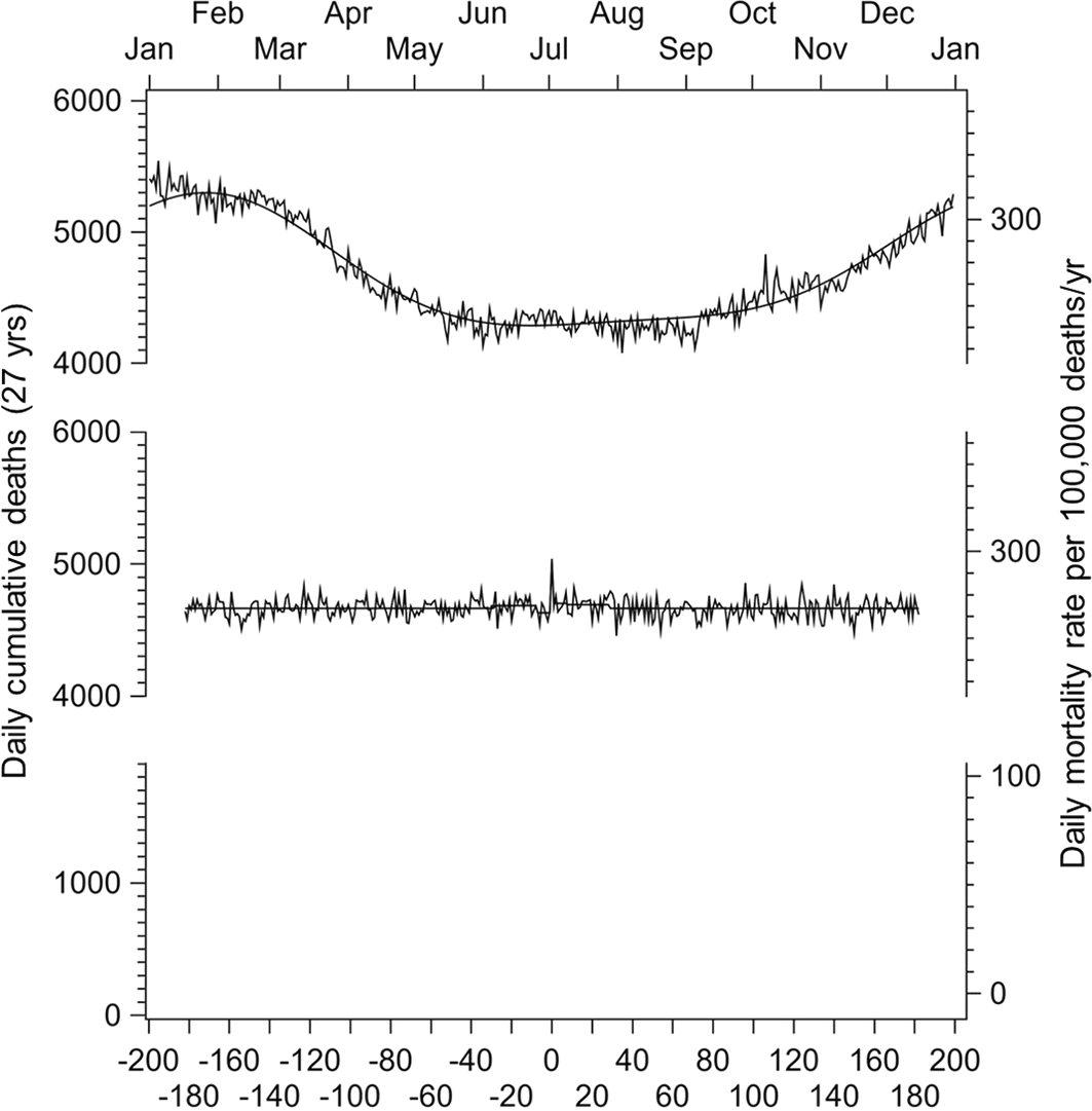
The jagged lines represent the observed daily deaths of the full analysis set cumulated over the 27 non-leap years from 1987 to 2022, the smooth lines depicting the model-based predictions. In the upper panel, the abscissa at the top of the graph represents the passage of 365 calendar days. In the lower panel, for the same data, the abscissa at the bottom represents the day of death minus the day of birth.

In the lower part of Figure 1, where the same data is shown over the interval between the day of death and the day of birth, a peak is discernible in the middle of the graph when both days coincide. Across all years, an average of 130,518 deaths occurred over a period of, for comparison, 28 days during the reference period, compared to 130,724 deaths in the 28 days before and 131,407 deaths in the 28 days after the birthday. Centering the latter two counts by subtracting the reference period count obtains 206 and 889 excess deaths in the 28 days before and after the birthday, respectively. With 18.8 percent of the excess cases observed in the four weeks before the birthday and 81.2 percent in the four weeks after, the likelihood of a symmetrical distribution of deaths around the birthday is less than 0.01 percent, strongly pointing towards higher mortality after the birthday than before in the full analysis set. Figure 2 shows the period from 30 days before to 30 days after the birthday, depicting both the observed and the predicted rates as daily mortality rates per 100,000 deaths per year.

Figure 2. Daily mortality rates from 30 days before to 30 days after the birthday.

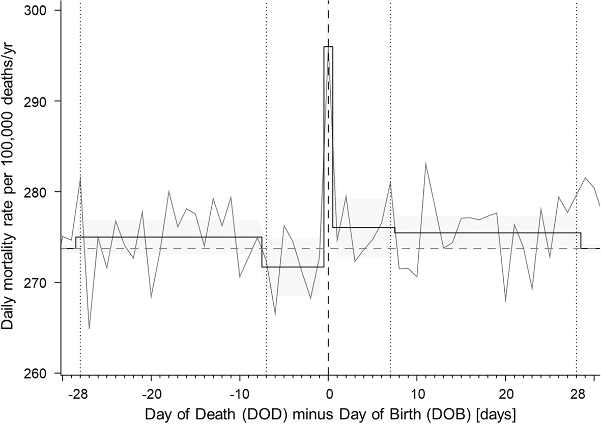
The smooth line segments (and 95% confidence intervals) indicate the predicted daily mortality, the jagged line the observed daily rates. For periods B[-28,-8], B[-7,-1], B[1,7], and B[8,28], but not for period B[0] (the birthday itself ), the confidence interval around the predicted rates covers the mortality rate predicted for the reference period C[-182,-29;29,182], the level of which is visible for 29 and 30 days before and after the birthday.

When a comparison-wise false-positive error level of five percent is adopted to explore the 95% confidence intervals for potential effects, Figure 2 suggests that the impact of the birthday itself on the model likelihood exceeds what would be anticipated from random variation. Conversely, while the predicted daily mortality rates for the periods preceding and following the birthday suggest a pattern, the associated 95% confidence intervals cover the predicted reference period level.

Demographic groups

Importantly, B period effects which might exist for different demographic or diagnostic groups could dilute or even cancel each other in the full analysis set. Table 2 thus provides an overview of the demographic subgroups for which regression analyses were conducted. The analysis sets are disjunctive within each demographic characteristic (sex, marital status, registered religious affiliation, year of death, and, when disregarding the 65+ years group, age) but not between them. For age, five disjunct strata are reported in Table 2: 18-64 years and four 10-year age groups covering the range between 65 and 104 (with the largely redundant 65+ group included mainly to facilitate comparisons with published mortality statistics that often dichotomize age at 65 years).

Table 2. Characteristics of the cases contained in the full analysis set (ALL) and in various demographic subgroups.

Analysis set	N	Prop. Mort. [%]	Winter Exc Mort. [%]	Min./Max. Mortality [date]	Men [%]	Mar. [%]	Rel. Affil. [%]	Age [y]	D- Sun. [%]	YOD 1995+ [%]
ALL	1,702,865	100.0	36.0	03AU/05JA	49.0	39.9	87.5	77.7	13.9	78.5
Women	868,087	51.0	42.5	05SE/05JA	0.0	22.5	89.0	81.0	14.0	79.3
Men	834,778	49.0	31.8	09AU/01JA	100.0	58.0	85.8	74.4	13.9	77.7
Married	679,868	39.9	32.8	03AU/10JA	71.2	100.0	87.1	73.8	13.9	77.4
Not Married	1,022,997	60.1	41.6	03JN/05JA	34.3	0.0	87.7	80.4	14.0	79.3
Rel. Affil.	1,489,272	87.5	37.8	03AU/05JA	48.1	39.8	100.0	78.2	14.0	76.3
No Rel. Aff.	213,593	12.5	48.1	14JN/27DE	55.4	40.9	0.0	74.4	13.7	94.0
Age 18-64	272,599	16.0	24.0	05AU/05JA	65.2	53.2	81.3	51.7	14.0	73.9
Age 65+	1,430,266	84.0	39.9	03AU/05JA	45.9	37.4	88.6	82.7	13.9	79.4
Age 65-74	272,010	16.0	39.1	25JL/26JA	61.8	58.9	85.3	70.0	13.7	75.0
Age 75-84	509,282	29.9	43.5	03AU/05JA	51.7	45.8	88.9	80.0	13.9	75.9
Age 85-94	552,932	32.5	53.2	20AU/05JA	36.7	24.2	90.0	89.0	14.0	82.9
Age 95-104	95,335	5.6	88.9	05JL/11DE	24.0	8.1	88.9	97.0	14.1	90.0
YoD < 1995	365,819	21.5	51.4	18AU/03JA	50.9	42.0	96.5	74.9	14.1	0.0
YoD 1995+	1,337,046	78.5	37.8	03AU/05JA	48.5	39.4	85.0	78.5	13.9	100.0

The data reveal several notable and straightforward patterns. For example, the largest winter excess mortalities occurred in the 85-94 (52.3%) and 94-104 (88.9%), the lowest in the 18-64 (24.0%) years of age groups, suggesting an increasing vulnerability to low ambient temperatures with age; the proportion of cases with no registered religious affiliation substantially increased from 1995 onwards compared to earlier years, indicating a trend toward secularization; and the proportion of deaths occurring from 1995 onwards increases with the age of the deceased, indicating a secular lengthening of life expectancy.

To address the main topic of comparing mortality rates in the B periods and the reference period C, Table 3 presents the daily mortality rate predictions and mortality rate ratios of the B periods relative to the C period, along with 95% confidence intervals. Likelihood ratio tests indicated only marginal contributions of B periods in women (p=0.07) and in deceased with no registered religious affiliation (p=0.25). Otherwise, with the exception of married deceased (p=0.01), p-values were smaller or much smaller than 0.001.

Table 3. Daily mortality rates (MR) per 100,000 deaths/y and mortality rate ratios (MRR) (italics) stratified by demographic characteristics, along with 95% confidence intervals, for periods B[from,to] days away from birthday, and reference period C 182 to 29 days before and 29 to 182 days after birthday.

Model	B[-28,-8]	B[-7,-1]	B[0]	B[1,7]	B[8,28]	C[-182,-29; 29,182]
ALL	275.0 [273.14;276.85]	271.7 [268.50;274.88]	296.0 [287.17;304.78]	276.0 [272.82;279.25]	275.5 [273.60;277.31]	273.7 [273.25;274.22]
	1.00 [0.998;1.012]	0.99 [0.981;1.004]	1.08 [1.049;1.114]	1.01 [0.997;1.020]	1.01 [0.999;1.013]
Women	140.2 [138.90;141.52]	138.9 [136.67;141.18]	148.2 [142.06;154.38]	139.7 [137.44;141.96]	139.8 [138.54;141.15]	139.6 [139.26;139.95]
	1.00 [0.995;1.014]	1.00 [0.979;1.012]	1.06 [1.018;1.107]	1.00 [0.984;1.017]	1.00 [0.992;1.011]
Men	134.8 [133.50;136.07]	132.8 [130.56;134.98]	147.8 [141.59;153.91]	136.3 [134.10;138.58]	135.6 [134.32;136.89]	134.1 [133.80;134.47]
	1.00 [0.995;1.015]	0.99 [0.973;1.007]	1.10 [1.056;1.149]	1.02 [1.000;1.033]	1.01 [1.001;1.021]
Married	109.7 [108.53;110.81]	107.9 [105.98;109.89]	115.0 [109.69;120.39]	112.0 [109.97;113.96]	109.3 [108.14;110.42]	109.3 [109.03;109.62]
	1.00 [0.992;1.014]	0.99 [0.969;1.006]	1.05 [1.004;1.102]	1.02 [1.006;1.043]	1.00 [0.989;1.010]
Not M.	165.3 [163.89;166.75]	163.8 [161.29;166.22]	180.9 [174.07;187.79]	164.1 [161.61;166.55]	166.2 [164.74;167.61]	164.4 [164.03;164.78]
	1.01 [0.997;1.015]	1.00 [0.981;1.011]	1.10 [1.059;1.143]	1.00 [0.983;1.013]	1.01 [1.002;1.020]
Rel. Aff.	240.1 [238.35;241.81]	236.8 [233.84;239.80]	260.0 [251.77;268.29]	241.4 [238.43;244.44]	240.9 [239.17;242.64]	239.4 [238.99;239.90]
	1.00 [0.995;1.010]	0.99 [0.977;1.002]	1.09 [1.052;1.121]	1.01 [0.996;1.021]	1.01 [0.999;1.014]
No Rel.	34.9 [34.39;35.44]	34.9 [33.96;35.79]	35.9 [33.48;38.40]	34.6 [33.69;35.52]	34.5 [34.02;35.07]	34.3 [34.16;34.43]
	1.02 [1.002;1.034]	1.02 [0.990;1.044]	1.05 [0.979;1.122]	1.01 [0.983;1.036]	1.01 [0.992;1.023]
18-64	45.6 [44.99;46.27]	46.4 [45.28;47.51]	47.9 [44.86;50.86]	42.5 [41.42;43.55]	42.0 [41.41;42.64]	43.8 [43.66;43.99]
	1.04 [1.026;1.056]	1.06 [1.033;1.085]	1.09 [1.026;1.163]	0.97 [0.945;0.994]	0.96 [0.945;0.974]
65+	229.4 [227.67;231.06]	225.3 [222.39;228.21]	248.1 [240.04;256.19]	233.6 [230.59;236.52]	233.4 [231.72;235.14]	229.9 [229.47;230.36]
	1.00 [0.990;1.005]	0.98 [0.967;0.993]	1.08 [1.045;1.115]	1.02 [1.003;1.029]	1.02 [1.008;1.023]
65-74	45.1 [44.46;45.73]	44.8 [43.74;45.93]	48.4 [45.38;51.40]	43.2 [42.13;44.28]	42.5 [41.88;43.11]	43.7 [43.57;43.90]
	1.03 [1.016;1.046]	1.03 [1.000;1.051]	1.11 [1.040;1.178]	0.99 [0.963;1.013]	0.97 [0.957;0.986]
75-84	83.8 [82.80;84.73]	83.4 [81.72;85.04]	85.4 [80.94;89.83]	80.3 [78.63;81.89]	80.7 [79.71;81.59]	81.9 [81.65;82.14]
	1.02 [1.011;1.035]	1.02 [0.998;1.039]	1.04 [0.990;1.098]	0.98 [0.960;1.000]	0.98 [0.973;0.997]
85-94	87.2 [86.22;88.19]	84.6 [82.93;86.30]	95.6 [90.87;100.34]	92.0 [90.27;93.79]	92.2 [91.16;93.19]	88.9 [88.61;89.13]
	0.98 [0.970;0.993]	0.95 [0.933;0.971]	1.08 [1.024;1.130]	1.04 [1.016;1.056]	1.04 [1.025;1.049]
95-104	13.2 [12.97;13.49]	12.4 [11.96;12.82]	18.6 [17.21;20.02]	17.9 [17.33;18.37]	17.9 [17.63;18.24]	15.3 [15.23;15.38]
	0.86 [0.847;0.882]	0.81 [0.782;0.839]	1.22 [1.128;1.312]	1.17 [1.133;1.201]	1.17 [1.152;1.193]
YD<95	58.6 [57.83;59.38]	58.7 [57.35;60.05]	69.5 [65.60;73.34]	60.0 [58.60;61.32]	58.8 [58.03;59.58]	58.8 [58.62;59.02]
	1.00 [0.983;1.010]	1.00 [0.975;1.021]	1.18 [1.117;1.249]	1.02 [0.996;1.043]	1.00 [0.986;1.013]
YD95+	216.4 [214.75;218.03]	213.0 [210.18;215.81]	226.5 [218.82;234.18]	216.1 [213.25;218.92]	216.7 [215.01;218.29]	214.9 [214.49;215.34]
	1.01 [0.999;1.015]	0.99 [0.978;1.004]	1.05 [1.019;1.090]	1.01 [0.992;1.019]	1.01 [1.000;1.016]

In all groups depicted in Table 3, mortality rate ratios larger than one were found for B[0], the confidence intervals covering unity only in the no registered religious affiliation and the 75-84 years of age strata. A small pre-birthday MRR increase of about two percent was found in deceased with no registered religious affiliation for B[-28,-8]. Small post-birthday mortality rate ratio increases (of about one to two percent each) were found in male and in unmarried deceased for B[8,28] and in married deceased for B[1,7]. More pronounced effects were found regarding age. Based on the 95% confidence intervals’ lack of covering unity, increased MRRs were observed for B[-28,-8] and decreased MRRs for B[8,28] in the 18-84 years of age range. Additionally, in the 18-64 years stratum, the MRRs for B[-7,-1] were increased and those for B[1,7] decreased. Conversely, in the two oldest age strata of the 85-104 years range, the reverse pattern was found, with MRRs decreased pre-birthday during B[-7,-1] and B[-28,-8], and increased post-birthday during B[1,7] and B[8,28]. For B[-7,-1], B[1,7], and B[8,28], this pattern is also visible in the broader 65+ years of age group.

Disregarding the full analysis set and, to avoid overlap, the 65+ years of age group, Table 3 contains 95% confidence intervals for 65 MRRs, of which 31 do not cover the null-effect mortality ratio of one, where, by chance, only slightly more than three (3.25) would be expected. When also disregarding the B[0] period, 20 out of 52 intervals do not cover unity, while only between two and three (2.6) would be expected.

Figure 3 depicts the observed and predicted daily mortality rates over the five B periods for the strata of sex, marital status, year of death, registered religious affiliation, and for the age groups 18-64, 65-74, 75-84, 86-94, and 95-104 years. It can be seen that (as with the corresponding MRRs contained in Table 3) the estimates are more precise for longer than for shorter B periods, the underlying numbers of cases being smallest for B[0], and consequently the confidence intervals the widest. In the year of death strata (<1995 and 1995+), in men and women, in married and unmarried deceased, as well as in deceased with a registered religious affiliation, B[0] excess mortality is visible, which in married deceased also obtains in B[1,7] and in unmarried deceased and in men in B[8,28]. In deceased with no registered religious affiliation, no association with predicted mortality is discernible from the week before birthday onwards, including the birthday itself, with observed mortality rates exhibiting considerable variability in this group.

Figure 3. Daily mortality rates from 30 days before to after the birthday for demographic strata.

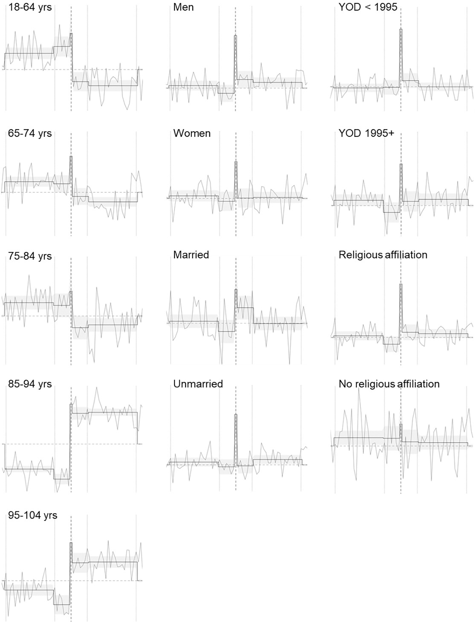
The smooth lines (with 95% CIs) show predicted rates for B[-28,-8], B[-7,-1], B[0], B[1,7], and B[8,28], as indicated by dotted vertical lines; the jagged lines show observed rates. Reference period rates appear at the edges (29 and 30 days before and after birthday), with axes omitted to focus on the form of the predicted mortality trajectories.

With regard to the five disjunct age groups, a two-cluster solution of the normalized B period mortality rate predictions confirmed the MR patterns of Table 3, with age groups 18-64, 65-74, and 75-84 years forming one cluster and age groups 85-92 and 95-104 another. In the three younger age groups, distinct pre-birthday and birthday excess MRs are visible, succeeded by a reduction in MRs in the weeks after the birthday. Conversely, the two older age groups show a distinct pattern of reduced MRs before birthdays, followed by increased rates on birthdays and in the weeks that follow.

Diagnostic groups

Other than with demographic strata, all cause of death categories depicted in Table 4 are disjunctive. Of the 1,702,865 deceased of the full analysis set, 1,534,761 died of an underlying cause of death that falls into one of the 13 categories of major causes of death, rendering the combined proportionate mortality 90.1 percent. The proportionate mortalities of cardiovascular diseases and of cancer were 25.4 and 35.5 percent, respectively, the two diagnostic categories together accounting for 60.9 percent of all deaths. Other causes with proportionate mortalities of at least one in twenty decedents were respiratory diseases (6.4%), dementia (5.2%), and mental and behavioral disorders (5.0%). The smallest underlying cause of death category was COVID-19, with 8,125 cases contained in the analysis set, corresponding to a proportionate mortality of 0.5 percent.

Table 4. Characteristics of 1,534,761 cases with underlying cause of death in one of the 13 major cause of death categories.

Analysis set	N	Prop. Mort. [%]	Winter Exc Mort. [%]	Min./Max. Mortality [date]	Men [%]	Mar. [%]	Rel. Affil. [%]	Age [y]	D-Sun. [%]	YOD 1995+ [%]
Infections	16,837	1.0	125.8	17DE/21FE	52.2	38.0	86.3	73.1	14.1	85.7
Cancer	432,703	25.4	22.4	01JN/26NO	55.0	54.3	87.0	72.9	14.0	77.5
Mental-Behav.	85,682	5.0	97.0	11JN/10MR	34.2	25.0	86.6	84.7	13.6	97.6
Dementia	88,659	5.2	106.3	11JN/04MR	30.1	27.5	86.8	87.1	13.6	99.6
Circulatory	604,231	35.5	51.3	30AU/05JA	45.5	35.2	90.7	81.9	14.0	73.1
Respiratory	108,452	6.4	164.2	05SE/14FE	54.4	37.9	88.9	80.9	13.9	76.4
Diabetes	35,839	2.1	142.9	24MY/21JA	43.1	33.1	91.3	80.0	13.7	77.6
Genitourinary	21,911	1.3	164.7	20SE/16JA	47.1	35.0	88.0	83.3	14.1	83.0
Accident	65,750	3.9	68.4	04MY/25JN	56.2	34.0	85.7	68.4	14.6	71.3
Transp. Accid.	12,812	0.8	294.1	25FE/14SE	75.4	42.5	85.0	49.5	15.0	59.4
COVID-19	8,125	0.5	4'750.0	03JL/07JA	55.1	41.1	70.5	82.4	14.1	100.0
Suicide	42,792	2.5	173.2	25DE/01JL	64.5	40.6	72.8	59.0	10.5	79.2
Assisted Suic.	10,968	0.6	4'700.0	25DE/22NO	42.1	36.9	58.6	77.3	2.5	100.0

Winter excess mortality, while present in all major cause of death categories, was rather more heterogeneous than across the demographic groups. While for cancer the excess was 22.4 percent, it was 47.5-fold for COVID-19. For assisted suicide, the winter excess mortality was 47-fold compared to 1.7-fold for suicide, the former peaking in November and the latter in July. There were some similarities between suicides and assisted suicides, both having occurred least frequently on 25 December and rarely on Sundays, in particular (and quite possibly for administrative reasons) assisted suicide. The dissimilarities are, however, more impressive (even if assisted suicide has been coded separately only as of 1995): Suicides were, compared to assisted suicides, younger (59.0 vs. 77.3 years), more often religiously affiliated (72.8% vs. 58.6%), married (40.6% vs. 36.9%), and male (64.5% vs. 42.1%).

Short of confirmatory testing, exploratory likelihood ratio p-values provide some indication of the level of statistical support for B period mortality rate effects (although the evidentiary significance of p-values is compromised by their notorious dependence on sample size, with statistical power increasing and p-values decreasing as group size increases). The likelihood ratio test p-value of the B period indicator was < 0.05 for mental and behavioral causes, < 10⁻² for respiratory diseases and for assisted suicide, and < 10⁻³ for suicide and for cardiovascular diseases. It exceeded the 0.05 threshold (a prevalent convention in dichotomous confirmatory assessments) for accidents (0.08), transport accidents (0.11), diabetes (0.13), cancer (0.20), dementia (0.21), infections (0.23), genitourinary diseases (0.39), and COVID-19 (0.52). The rather large likelihood of the B periods not being substantially predictive of mortality in COVID-19 is consistent with the low overall proportionate mortality of 0.5 percent (8,125 cases) in this group. Similarly, the proportionate mortality was at one percent or below in infections (1.0%, 16,837 cases) and transport accidents (0.8%, 12,812 cases), and between one and barely above two percent in genitourinary diseases (1.3%, 21,911 cases) and diabetes (2.1%, 35,839 cases). The only two diagnoses with both proportionate mortalities above these levels and relatively low B period predictiveness likelihoods of about 20 percent were dementia (5.2%, 88,659 cases) and cancer (25.4%, 432,703 cases).

Table 5 presents the predicted daily mortality rates and mortality rate ratios of the B periods relative to the C period, along with 95% confidence intervals, for each of the 13 COD categories. As can be seen, for dementia and cancer, their low B period predictiveness is consistent with the B period-specific mortality rate ratio findings, all 95% confidence intervals covering the no-effect level of one for cancer, and for dementia only one excess mortality (during B[8,28] of about 3%) inconsistent with no effect.

Table 5. Daily mortality rates (MR) per 100,000 deaths/y and mortality rate ratios (MRR) (italics) stratified by major cause of death categories, along with 95% confidence intervals, for periods B[from,to] days away from birthday, and reference period C 182 to 29 days before and 29 to 182 days after birthday.

Model	B[-28,-8]	B[-7,-1]	B[0]	B[1,7]	B[8,28]	C[-182,-29; 29,182]
Infctn.	2.7 [2.63;2.75]	2.8 [2.65;2.87]	2.9 [2.57;3.18]	2.7 [2.60;2.82]	2.9 [2.86;3.00]	2.7 [2.68;2.71]
	1.00 [0.974;1.024]	1.02 [0.983;1.068]	1.07 [0.960;1.188]	1.01 [0.965;1.049]	1.09 [1.061;1.113]
Cancer	69.8 [68.92;70.64]	70.7 [69.18;72.18]	73.3 [69.25;77.33]	68.7 [67.23;70.19]	69.3 [68.43;70.15]	69.6 [69.39;69.84]
	1.00 [0.990;1.015]	1.02 [0.994;1.037]	1.05 [0.996;1.113]	0.99 [0.966;1.009]	1.00 [0.983;1.008]
Mental	13.7 [13.43;13.93]	13.5 [13.04;13.91]	13.6 [12.46;14.79]	13.4 [12.97;13.84]	14.4 [14.11;14.63]	13.8 [13.70;13.84]
	0.99 [0.975;1.013]	0.98 [0.947;1.011]	0.99 [0.908;1.078]	0.97 [0.942;1.006]	1.04 [1.024;1.064]
Demen.	14.4 [14.14;14.67]	13.9 [13.42;14.32]	14.6 [13.35;15.78]	14.4 [13.95;14.86]	14.7 [14.43;14.96]	14.2 [14.16;14.30]
	1.01 [0.993;1.032]	0.97 [0.943;1.007]	1.02 [0.941;1.113]	1.01 [0.980;1.045]	1.03 [1.014;1.052]
Circul.	97.3 [96.27;98.38]	96.8 [94.98;98.63]	107.6 [102.55;112.73]	99.0 [97.11;100.80]	97.9 [96.81;98.93]	97.1 [96.82;97.37]
	1.00 [0.991;1.014]	1.00 [0.978;1.016]	1.11 [1.057;1.162]	1.02 [1.000;1.039]	1.01 [0.997;1.019]
Respir.	17.9 [17.63;18.24]	16.8 [16.25;17.27]	18.6 [17.14;19.98]	17.8 [17.26;18.31]	17.9 [17.61;18.22]	17.4 [17.31;17.47]
	1.03 [1.013;1.050]	0.96 [0.935;0.994]	1.07 [0.988;1.152]	1.02 [0.993;1.054]	1.03 [1.013;1.049]
Diabet.	5.5 [5.33;5.57]	5.5 [5.31;5.73]	5.8 [5.19;6.32]	5.9 [5.65;6.08]	5.7 [5.60;5.85]	5.8 [5.76;5.83]
	0.94 [0.919;0.962]	0.95 [0.917;0.990]	0.99 [0.900;1.097]	1.01 [0.975;1.051]	0.99 [0.966;1.010]
Gn-Urin.	3.6 [3.51;3.68]	3.4 [3.22;3.49]	2.9 [2.54;3.22]	3.4 [3.28;3.56]	3.4 [3.35;3.51]	3.5 [3.51;3.56]
	1.02 [0.993;1.042]	0.95 [0.910;0.989]	0.81 [0.724;0.916]	0.97 [0.929;1.009]	0.97 [0.946;0.993]
Accident	10.3 [10.05;10.46]	10.3 [9.98;10.69]	11.5 [10.46;12.44]	11.1 [10.71;11.45]	10.8 [10.59;11.01]	10.6 [10.52;10.63]
	0.97 [0.949;0.989]	0.98 [0.944;1.012]	1.08 [0.993;1.181]	1.05 [1.013;1.084]	1.02 [1.001;1.042]
Tr. Acc.	1.9 [1.85;1.95]	1.9 [1.82;1.99]	2.5 [2.21;2.72]	2.2 [2.13;2.31]	2.1 [2.02;2.12]	2.1 [2.06;2.08]
	0.92 [0.895;0.943]	0.92 [0.880;0.962]	1.19 [1.075;1.320]	1.07 [1.030;1.119]	1.00 [0.973;1.024]
COV19	1.4 [1.35;1.41]	1.4 [1.34;1.43]	1.4 [1.29;1.53]	1.4 [1.40;1.49]	1.3 [1.29;1.34]	1.3 [1.29;1.30]
	1.07 [1.043;1.088]	1.07 [1.031;1.105]	1.09 [0.996;1.187]	1.11 [1.076;1.151]	1.01 [0.992;1.036]
Suicide	7.0 [6.90;7.19]	6.9 [6.62;7.11]	10.0 [9.19;10.77]	6.9 [6.61;7.10]	7.0 [6.84;7.12]	6.9 [6.82;6.90]
	1.03 [1.005;1.049]	1.00 [0.965;1.038]	1.46 [1.345;1.576]	1.00 [0.964;1.036]	1.02 [0.996;1.040]
Ass. S.	1.9 [1.85;1.92]	1.8 [1.69;1.82]	3.1 [2.83;3.28]	1.7 [1.63;1.76]	1.8 [1.80;1.88]	1.7 [1.74;1.76]
	1.08 [1.054;1.102]	1.00 [0.966;1.041]	1.75 [1.623;1.878]	0.97 [0.933;1.006]	1.05 [1.027;1.074]

Regarding birthday and post-birthday period MRRs, mortality increases exclusively during B[8,28], as seen with dementia, were also found for infections (of about 9%), mental and behavioral diseases (4%), and respiratory diseases (3%). Excess mortality only during B[1,7] was found in COVID-19 (11%) and only on B[0] in circulatory diseases (11%) as well as in suicides (46%). Increases were found for both B[0] and B[1,7] in transport accidents (19% and 7%), for both B[0] and B[8,28] in assisted suicide (75% and 5%), and for both B[1,7] and B[8,28] in accidents (5% and 2%). Lower than expected mortality on or after the birthday was found on B[0] as well as during B[8,28] in genitourinary diseases (-19% and -3%).

Pre-birthday , excess mortality was found during B[-28,-8] for respiratory diseases (3%), suicide (3%), assisted suicide (8%), and COVID-19 (7%), for the latter also during B[-7,-1] (7%). Lower than expected mortality only during B[-7,-1] was found in respiratory diseases (-4%) and in genitourinary diseases (-5%), only during B[-28,-8] in accidents (-3%), and during both pre-birthday periods in diabetes (between -5% to -6%) and transport accidents (-8%).

Of the 65 MRR 95% confidence intervals depicted in Table 5, 27 indicate that the birthday period mortality ratios deviate systematically from what would be expected from the reference period rates. This number is more than eight times higher than the 3.25 false positives expected by chance alone. Disregarding the B[0] period, 22 out of 52 MRRs show mortality rate deviations from the reference period that are not consistent with merely random variation, compared to the 2.6 false positives expected by chance. Of the twelve pre-birthday intervals that deviate from expectations, seven indicate a decreased mortality rate, while increased pre-birthday mortality was only found in respiratory diseases, COVID-19, accidents, and transport accidents. In contrast, with the exception of genitourinary diseases, all of the 15 marked birthday and post-birthday period effects indicate increased mortality.

Figure 4 illustrates the observed and predicted daily mortality rates across the five B periods for each of the 13 COD categories. The six-cluster solution resulted in three clusters combining multiple COD categories, alongside three distinct diagnostic categories (respiratory diseases, genitourinary diseases, COVID-19) that were not combined with others. The three multi-category clusters are depicted in the three columns above the bottom row that shows the three solitaire COD categories. It is important to recall that the clustering was solely based on the phenotypic patterns of normalized B period mortality rates, with no consideration of underlying mechanistic similarities or differences whatsoever.

Figure 4. Birthday period mortality rates by major cause of death category.

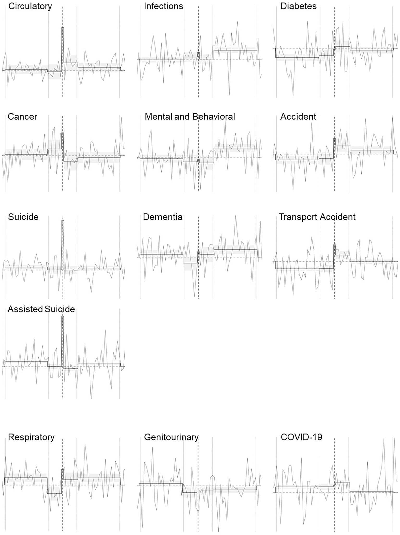
Daily mortality rates (smooth lines) and their 95% confidence intervals across the five B periods, as predicted by the 13 major cause of death category-specific Poisson models. The observed daily death rates are shown in the background (jagged curves). In each panel, the central vertical dotted line indicates the birthday, the vertical lines to its left and right ±7 and ±28 days before and after the birthday. The six-cluster solution of the normalized rates yielded three clusters with multiple major cause of death categories combined (three columns in the upper part). These contain (i) circulatory diseases, cancers, suicides, and assisted suicides, (ii) infections, mental and behavioral diseases, and dementia, and (iii) diabetes, accidents, and transport accidents. The proportionate mortality (PM) of these clusters is 64.1, 11.2, and 6.7 percent, respectively. Respiratory diseases (6.4% PM), genitourinary diseases (1.3% PM), and COVID-19 (0.5% PM) were retained as stand-alone causes of death categories (bottom row of panels).

The left-hand column of Figure 4 depicts the cluster comprising circulatory diseases, cancer, suicide, and assisted suicide, combining two somatic and two behavioral COD categories. An increased mortality rate is visible for all four causes at B[0], with cancer showing the least pronounced peak. The two behavioral categories also exhibit a pre-birthday mortality increase during B[-28,-8], and assisted suicide additionally shows a post-birthday increase during B[8,28].

The middle column shows the cluster that comprises infections, mental and behavioral diseases, and dementia. In neither of these COD categories a B[0]-specific increased (or decreased) mortality rate is discernible, whereas all three groups show a B[8,28] post-birthday mortality rate increase.

The right-hand column shows the cluster that includes diabetes, accidents, and transport accidents. The three constituent COD categories exhibit reduced pre-birthday mortality, with patterns that, when mirrored across the midpoint of the reference-period risk level, approximately reflect those observed in the middle column cluster.

The B period mortality patterns for respiratory and for genitourinary diseases are consistent with a short-term displacement effect that precedes the birthday by a few days. In contrast, for COVID-19, elevated mortality rates were found throughout the birthday period, with only a marginal additional effect associated with the birthday itself.

Resampling was done on the three clusters that comprise multiple major causes of death categories, the method not relying on parametric or paradigmatic analyses (as in regression models with pre-specified birthday periods). The resulting mortality variations in proximity to the birthday are contained in Figure 5.

Figure 5. Daily and smoothed boostrap averages of observed minus predicted deaths over the birthday period.

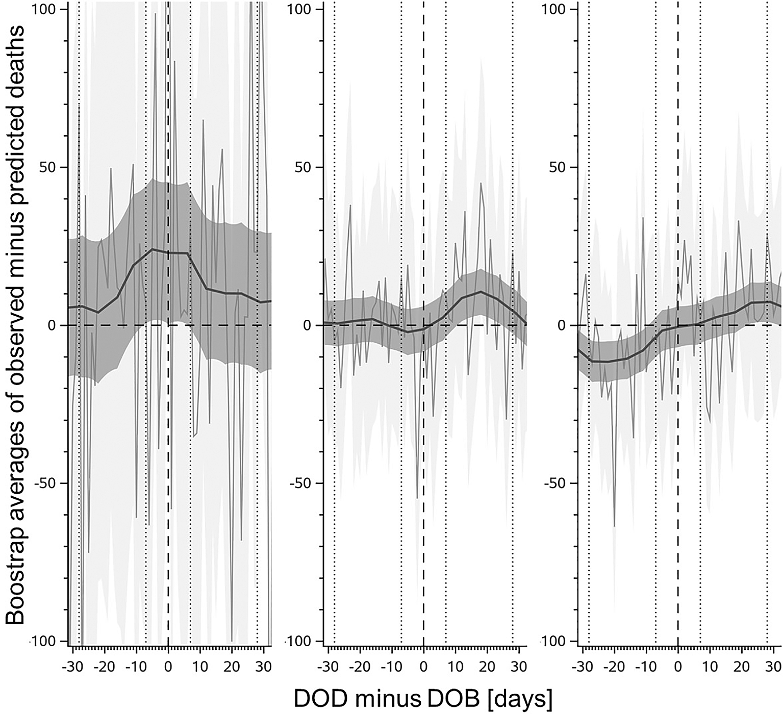
The jagged curves in the background represent the daily bootstrap averages, accompanied by 95% confidence intervals. Resampling of 100,000 cases each was conducted separately for the three multi-category COD clusters shown in Figure 4. Left panel: Circulatory diseases, cancers, suicides, and assisted suicides, characterized by increased mortality on the birthday itself. Middle panel: Infections, mental and behavioral diseases, and dementia, characterized mainly by increased mortality in the weeks following the birthday. Right panel: Diabetes, accidents, and transport accidents, characterized mainly by reduced pre-birthday mortality. The smooth LOESS curves and their 95% prediction bands in the foreground are schematic representations of the forms of the cluster-specific trajectories over the birthday period rather than isomorphic depictions of the distribution of actual average mortality deviations from expected levels. This is due to the low-pass filter properties of the method that attenuates short-term variations and induces temporal smearing. This is particularly visible in the left panel, where the effect on the birthday itself, while visible, is clearly less peaked and of smaller amplitude than the average of the observed minus expected differences on B[0] (293 cases). It is noticeable that the variability of the daily averages over the birthday period is substantially larger for the COD categories depicted in the left panel, where mortality effects are mostly restricted to the birthday itself.

As with the preceding model-based analyses, the resampling results point to systematic birthday-related mortality variations, with the pre- and post-birthday mortality patterns differing both temporally and in magnitude from each other and from the birthday itself. Since resampling was done on combinations of COD categories both related and unrelated to direct behavioral causes, the mechanisms underlying the observed patterns are almost certainly more complex than the three major trajectories depicted in Figure 5 might suggest.

Sensitivity analyses

To explore the potential confounding of the observed associations between B period and mortality by age-related biases, the left panel of Figure 6 depicts the fundamental age-association of mortality, even if with the present data the phenomenon occurs ten age years later than what Roger had found in 1972 UK mortality data, the shift obviously reflecting a substantial secular increase in life expectancy over the last five decades. In the present data, up to the age of 85, the number of deaths increases. From age 86 onward, the trend reverses with a sharp decrease in the number of deaths for each subsequent year of age, reflecting the rapid shrinking of the risk sets of older age cohorts, as opposed to younger ones. As a consequence of this biphasic age-dependent mortality pattern, even in the absence of any other effect, the daily numbers of deaths must be expected to decrease in the age groups above 85 years over the 364 days following the last birthday. As is shown in the age group-specific scatter plots and regression lines in the right panel of Figure 6, this is indeed the case, the older age groups displaying a declining and the younger age groups an upward trend. This raises the question as to whether the observed birthday effects are entirely or partially age-related artifacts, including of what can be referred to as “ageing-gradient bias”.

Figure 6. Number of deaths by age and days after the last birthday.

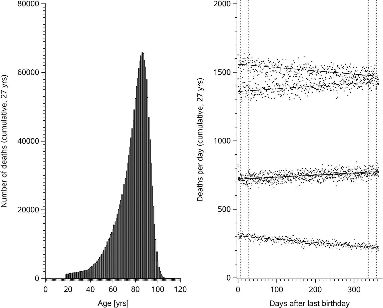
Left panel: Number of deaths by year of age, showing 65,752 deaths (3.86%) at a maximum of 86 years. Right panel: Age group-specific scatter plot of the number of daily deaths by days after the last birthday, with the linear regression lines ${\widehat{\mathrm{y}}}_{\mathrm{t}}$ = b₀+b₁t predicting the number of deaths per age group on day t after the last birthday. The total predicted number of deaths on day t is obtained by either summing the age group-specific predicted numbers for that day, by computing daily predicted numbers based on aggregated age group-specific regression parameters, or by regressing the total daily death count against the days elapsed since the final birthday without age group stratification. In the 85-94 (top) and the 95-104 years of age groups (bottom), the numbers of deaths per day decline after the last birthday, while they increase in the three younger age groups, the two groups 18-64 and 65-74 largely overlapping in the range of 500 to 1000 deaths per day. The total daily number of deaths ${\widehat{\mathrm{y}}}_{\mathrm{t}}$ = 4,648+0.0622t is rather stable over time, which aligns with Figure 1. As can be calculated from the overall regression equation, the mortality ratios of the five B periods are all 1, indicating that the age composition of the full analysis set and the combined age group-specific mortality age-gradients did not induce any B period effect. To introduce a one percent MRR increase in the most age gradient-sensitive off-birthday B period B[1,7] (due to its vicinity to t = 0), the slope of the regression equation would have to be multiplied by a factor of 4.23. Preserving the linear additivity of the age group-specific estimates, this slope factor would imply that in the 95-104 years of age group the number of daily predicted deaths would be negative for t ≥ 319.

As is confirmed in Table 6, age is obviously substantially important for mortality, the sensitivity parameter RR_AD increasing as mortality disbalance across the age groups increases. The more prominent levels of that parameter are consistent with fundamental relationships: Only 1.1 percent of married deceased were 95 years or older, suggesting that the chances of both spouses reaching such an advanced age were relatively small; prior to 1995, only 2.6 percent of the deceased were in that oldest age group, compared to 6.4 percent of those who died in 1995 or later, reflecting the increased life-expectancy of the population; only 0.3 percent of the transport accidents were 95 years or older, obviously reflecting reduced levels of mobility in that segment; only 1.3 percent of those who died with cancer as the underlying disease and only 1.2 percent of suicides reached an age of 95 or older, while other diagnoses were particularly rare in the 18-64 years of age-group, including dementia (0.7%) and genitourinary diseases (4.6%).

Table 6. Sensitivity analysis to estimate the maximum potential confounding by the uncontrolled factor age.

For each B period, RR^B_XA is the largest per age group ratio of the proportion of deaths among those dying in period X = B to the proportion among those dying in period X = C. It quantifies the imbalance of deaths between two contrasted X periods (the respective B period and the C period) across the five age groups. RR^B_AD is the largest ratio across periods X, where each ratio is calculated as the highest proportion of deaths to the lowest proportion among the five age groups within a specific period X. It quantifies the importance of the uncontrolled confounder age on the outcome.

Analysis set	B[-28,-8]		B[-7,-1]		B[0]		B[1,7]		B[8,28]
	RRXA	RRAD	RRXA	RRAD	RRXA	RRAD	RRXA	RRAD	RRXA	RRAD
ALL	1.04	6.59	1.07	6.83	1.12	5.80	1.16	5.81	1.16	5.85
Women	1.03	5.50	1.10	5.53	1.10	4.83	1.15	4.84	1.17	4.87
Men	1.04	13.95	1.05	16.25	1.25	11.50	1.21	11.54	1.18	11.62
Married	1.03	37.68	1.06	45.43	1.35	30.09	1.26	30.22	1.27	30.56
Not M.	1.04	5.46	1.08	5.65	1.09	4.79	1.16	4.80	1.15	4.83
Religion	1.03	6.63	1.06	6.87	1.17	5.87	1.14	5.88	1.17	5.92
No Rel.	1.05	6.46	1.08	6.96	1.08	6.88	1.31	5.35	1.09	5.34
YoD<95	1.03	14.75	1.05	15.08	1.24	12.82	1.15	12.85	1.24	13.01
YoD 95+	1.04	6.14	1.09	6.33	1.13	5.35	1.16	5.36	1.16	5.39
Infecti.	1.07	11.48	1.08	7.60	1.11	7.56	1.08	9.70	1.41	7.82
Cancer	1.06	29.19	1.08	34.45	1.75	23.20	1.13	23.21	1.16	23.36
Ment.-B.	1.05	9.16	1.15	9.09	1.19	10.09	1.09	9.20	1.21	11.05
Dement.	1.20	84.03	1.11	89.80	1.23	82.86	1.09	124.25	1.19	83.48
Circul.	1.05	6.34	1.06	6.73	1.17	5.63	1.17	5.91	1.18	5.73
Respir.	1.04	6.69	1.14	8.20	1.16	6.21	1.07	5.99	1.14	6.04
Diabetes	1.10	9.28	1.12	11.43	1.26	8.83	1.24	8.88	1.10	8.88
Gnitour.	1.07	10.78	1.14	9.62	1.36	23.00	1.53	9.59	1.29	10.29
Accident	1.03	8.02	1.07	9.93	1.06	6.90	1.23	6.75	1.10	6.77
Tsp. A.	1.06	268.90	1.27	262.45	1.23	266.24	1.40	261.82	1.03	516.00
CVD-19	1.27	5.63	1.17	5.64	1.66	5.62	1.13	6.40	1.25	5.63
Suicide	1.07	71.05	1.26	49.80	1.51	49.64	1.19	155.67	1.13	50.09
Ass. S.	1.19	10.45	1.28	8.57	1.55	8.53	1.20	23.67	1.10	8.59

In contrast to the anticipated, plausible, and largely profound levels of RR_AD, the importance of whether or not death occurred in a B period on the age of death, as quantified by the sensitivity parameter RR_XA, was generally small, in line with the flagrant implausibility of death occurring in a specific B period having any relevance to the age of death. As a consequence, half of the resulting bias factors were below 1.19 and three quarters below 1.19, the largest factor being 1.75 for cancer and B[0].

The mortality effects of birthday periods being substantially smaller than those of age per se, the conceptual sensitivity analysis focusing on confounding away from the null confirmed that all but the B[0] effect in assisted suicide could, in theory, be adjusted away by age. The two serious caveats of this assessment are, however, that it only holds for the most extreme confounding scenarios and that it entirely neglects false-negative findings by confounding towards the null. Applying the bias factors to the estimated MRRs of the 13 diagnostic categories indeed yielded the following numbers of de novo effects below/above expectations: 7/3 B[-28,-8], 5/8 B[-7,-1], 3/3 B[0], 7/5 B[1,7], and 9/4 B[8,28]. The large number of 54 purportedly overlooked effects in this evaluation underscores the sensitivity analysis as too extreme. Conversely, it is unlikely that most of the observed effects, while they could theoretically be adjusted away by age, are indeed false positives and would indeed vanish upon actual adjustment for age.

To complement the conceptual sensitivity analysis with an empirical assessment, the adjustment set of the original analysis (season and day of week) was replaced by age group, with 17-64 years as the reference category. Age was, as expected, generally associated with mortality in all demographic and diagnostic analysis sets. In the full analysis set, mortality rate ratios quantifying the effects of age group on the expected counts of deaths were found to be elevated for the 75-84 age group (1.87; 95%CI: 1.857, 1.880) and the 85-94 age group (2.03; 2.016, 2.041), but not for the 65-74 age group (1.00; 0.991, 1.005) or the 95+ age group (0.35; 0.349, 0.356). However, none of the original B period ratio estimates changed up to the fourth decimal place upon adjustment by age group, neither in the full analysis set nor in any of the demographic and diagnostic groups. The robustness of MRRs across adjustment sets indicates that, empirically, B period effects were independent of age. This is reflected in an extremely small value of Cramer’s V, quantifying the association between B period and age group, of 0.0094 in the full analysis set. Even in the diagnostic groups with the youngest and oldest mean age of the deceased there was no indication of an association between B period and age, with Cramer’s V values 0.0149 and 0.0153, respectively, for transport accidents and dementia.

The possible magnitudes of B period effects, would they solely depend on ageing, were quantified by simple linear regression analyses conducted for all demographic groups (except for age groups) and diagnostic groups. The coefficients were determined by regressing the daily number of deaths against days after the last birthday. From the coefficients and the respective time periods, the ageing-gradient bias was quantified by calculating purely ageing-based B period MRR estimates (which must necessarily be most pronounced for B[0], followed by the two seven-day periods directly before and after the birthday). With an accuracy of two decimal places, in all demographic groups, with the exception of women, the B[0] MRRs (and thus also those of the other four B periods) were all 1.00. In women, the value was slightly below 0.995. For most diagnostic groups, the B[0] MRRs were less than one percent (cancer, circulatory diseases, respiratory diseases, genitourinary diseases, accidents, transport accidents) or less than two percent (infections, mental and behavioral diseases, dementia, diabetes) away from unity. Most of the ageing-based MRRs found in the diagnostic groups could directionally not have contributed to the observed effects, two examples being mental and behavioral diseases and dementia, where the observed B[8,28] MRRs were above one while the age-based MRRs were below one. Three purely ageing-based effect estimates which were in the same direction as the observed effects contained in Table 5 were the B[8,28] effect for infections of 1.015 and the B[-28,-8] and B[-7,-1] effects for diabetes of 0.990 and 0.989, respectively. While these could slightly reduce the observed effects, they were clearly too small to eliminate them. Likewise, the purely ageing-based estimated B[0] effects for suicides and assisted suicides of 1.012 and 1.030, respectively, while slightly biasing the observed effects away from the null, are far too small to explain away the MRRs of 1.46 (suicide) and 1.75 (assisted suicide). The much smaller observed assisted suicide B[8,28] MRR of 1.05 is, according to its ageing-based counterpart of 1.027, possibly due to ageing bias. The only substantial ageing gradient effect was found for the smallest diagnostic group, COVID-19, where the two observed pre-birthday excess MRRs of 1.07 can be explained by the ageing-based B[-28,-8] and B[-7,-1] estimates of 1.073 and 1.079, respectively. For the observed COVID-19 B[1,7] post-birthday excess MRR this is naturally not the case, as the ageing-based MRR for that period was substantially less than one (0.921).

The observed numbers of births and deaths on the first 28 days of any month were assessed for heaping by comparing them (i) to the expected daily count (both of births and of deaths) of 55,984.6 (the total number of cases, 1,702,865, multiplied by 12 months and divided by 365 days), (ii) to the expected relative daily frequency (1/28), and (iii) to the observed mean numbers for days 1 to 28 of 56,068 [adjusted 95% CI: 55,289; 56,847] for births and 56,035 [95% CI: 55,256; 56,813] for deaths. Of the 56 assessed counts, only that of 59,083 births on day 1 exceeded the upper confidence interval limit of the corresponding mean, as well the expected frequency by 5.5 percent. The relative frequency of births on day 1 was 3.8 percent of all births of the first 28 days of any month, compared to the expected daily frequency of about 3.6 percent.

Among the 52,064 cases where the day of birth and the day of death in any month coincided (55,663 overall, without restriction to the first 28 days of any month), none of the 28 observed counts exceeded the average daily number of cases of 1,859 [adjusted 95% CI: 1,718; 2,001]. Nominally, the day 1 count of 1,976 cases exceeded the expected value of 1,840.6 ([12/365]² multiplied by the total number of cases, 1,702,865) by 7.4 percent. As with births alone, the relative frequency of all births and deaths coinciding on one of the first 28 days of any month was 3.8 percent for day 1, where again about 3.6 percent were expected.

Stratified by month, the proportion of births and deaths coinciding on day 1 among all such coincidences over the first 28 days ranged from 3.6 to 3.8 percent from February to December, with all multiplicity-adjusted 95% confidence intervals covering the above mean of 3.8 percent for day 1 of any month. In contrast, the corresponding day 1 proportion for January 1 was 4.4 [4.2-4.5] percent. If this indicates that the above-described heaping of births on day 1 of any month is largely a January phenomenon, then, in the present data, about one in 20 children born on December 31 might have been assigned January 1 as their day of birth, which is not entirely implausible. Despite the January 1 counts of cases with day of birth and death coinciding not materially exceeding the expected levels or the average of the first 28 days of any month, an additional sensitivity analysis was conducted by removing all 59,083 cases born on day 1, not only of December but of any month. The B[0] MRs and MRRs and their 95% confidence intervals of the four diagnostic groups clustered together for their pronounced B[0] mortality (circulatory diseases, cancer, suicide, and assisted suicide) remained virtually unchanged. The biggest change was seen in assisted suicide, where the MR remained at 3.1 [2.88-3.33] and the MRR increased from 1.75 to 1.77 [1.64-1.90].

Discussion

The full analysis set comprised a total of 1,702,865 deaths in the adult Swiss resident population through the 27 non-leap years from 1987 to 2022. The Poisson model, regressing daily mortality counts on categorized days between death and last birthday, adjusting for seasonality and day of week, fitted the data well. Less deaths occurred on Sundays than on weekdays and the typical northern-hemispheric seasonal variation in mortality is clearly visible, except in those dying from cancer and before their mid- to late 60s. 5,040 deaths (0.296%) occurred on the birthday of the deceased, exceeding the 4,665 deaths (0.274%) that would be expected if deaths were evenly distributed across the 365 days centered around the last birthday. The birthday excess mortality of 375 deaths corresponds to a rate of 22 additional deaths per 100,000 deaths per year. Focusing on the birthday, this represents an eight percent increase in deaths on birthdays compared to what would be expected, such that out of approximately 13 individuals who die on their birthday, one death is attributable to the birthday itself.

There were 206 and 889 excess deaths, respectively, in the 28 days before and after the birthday, indicating substantial asymmetry of deaths around the birthday, with higher mortality after than before. As birthday period-related effects that might exist for different demographic or diagnostic groups could dilute or even cancel each other out in the full analysis set, stratified analyses were conducted. In all demographic strata, with the exception of deceased with no religious affiliation and in the 75-84 years of age group, increased mortality on the birthday itself was found, with excess mortalities about twice as pronounced in men and unmarried persons than in women and in married persons. In age groups 85 years and older, a clearly discernible pre-birthday dip was followed by a post-birthday excess mortality, that pattern being in line with stochastic mechanisms related to age-dependent ageing-related mortality gradients, as proposed by Roger (1977).

1,534,761 cases died of one of 13 categories of underlying causes of death, corresponding with a combined proportionate mortality of 90.1 percent, with cancer and cardiovascular causes accounting for 60.9 percent of all deaths. Increased mortality on the birthday itself was found for cardiovascular causes of death, transport accidents, suicides, and assisted suicides. Reduced pre-birthday along with increased post-birthday mortality, in a manner consistent with mortality gradients related to ageing, was only found for accidents and transport accidents, while for diabetes and genitourinary diseases pre-birthday mortality deficits were found but no post-birthday excesses. Reduced mortality was also found for genitourinary diseases on the birthday itself as well as in the weeks after the birthday. Exclusively excess mortality was found for infectious diseases, mental diseases, and dementia in the weeks after the birthday, for suicides before and on the birthday, and before, on, as well as after the birthday for assisted suicides. While respiratory and genitourinary diseases as well as COVID-19 were not combined with other major causes of death categories, three clusters containing multiple cause of death categories were formed; one containing circulatory diseases, cancer, suicides, and assisted suicides, characterized by above-expectation mortality mainly on the birthday itself; one containing infectious diseases, mental and behavioral diseases, and dementia, characterized mainly by post-birthday excess mortality; and one containing diabetes, accidents, and transport accidents, characterized mainly by pre-birthday mortality deficits and, in the case of accidents and transport accidents, also by a short-term mortality increase commencing with the birthday.

Given that systematic administrative errors, as well as stochastic mechanisms, could in principle introduce artificial mortality patterns in sync with the birthday period, a thorough investigation into these possibilities was conducted. Our investigations into the registration procedures ruled out the possibility that the "birthday effects" (rather than a single effect only on the birthday itself ) observed in our data could be due to administrative errors; civil registration records in Switzerland are established at birth or at the time of registration in the country, not at or after death. When a person dies, the relevant parts of the civil registration records are automatically transferred to our mortality database, independent of and prior to the information subsequently provided with the death certificate. Furthermore, the mortality variations observed across strata, including on the birthday itself, cannot be explained by administrative biases. Why, for instance, would the birthday mortality rate be elevated for cardiovascular diseases but not for genitourinary diseases? With regard to heaping, we found an above-expectation frequency of births occurring on the first day of a month, the effect basically stemming from more than expected births recorded on firsts of January. A sensitivity analysis removing all births on a first of a month did not, however, indicate any material effect on the estimates.

Investigating the potential bias due to ageing-gradient effects as described by Roger (1977), implying reduced mortality before and increased mortality after the birthday, revealed that while, in particular in the 85-94 and 85-104 age groups, monotonous mortality decline after the birthday did obtain, assessing bias factors to quantifying the maximum degree of systematic distortion of mortality rate ratios were not deemed to support the notion of the estimated effects to be due to confounding by age. This was confirmed by directly adjusting the estimates by age group (instead of by season and day of week), which left the effect estimates unchanged, both overall as well as in the demographic and diagnostic strata. Furthermore, a linear regression analysis estimating the statistical effect of ageing on the daily numbers of deaths demonstrated that our findings could generally not be explained stochastically through ageing-gradient bias. The exceptions to this were the pre-birthday excess mortality observed in COVID-19 and the excess in assisted suicides in the weeks after the birthday, with the latter being of marginal magnitude and the former observed in the smallest cause of death category. These findings demonstrate that the results are robust against the investigated sources of systematic error, which is in line with the results obtained by the main analysis itself: Deficit and excess mortality patterns across birthday-related periods varied strongly across diagnostic groups, with no consistent pattern of stronger effects in periods closer to the birthday compared to those further away, which would be, however, just what aging gradients would induce.

Concerning the question whether the observed effects are artificial or psychogenic, our analyses clearly indicate the latter. This is not to suggest that the estimated quantities are entirely free from some degree of systematic error, but rather that any such error is highly unlikely to result in material bias. Overall, we found compelling evidence that the proximity to a person's birthday is indeed associated with mortality variations. While, overall, mortality tends to be higher in the period of four weeks before to four weeks after the birthday, with a pronounced peak on the birthday itself and mortality after the birthday higher than before, the heterogeneity of this pattern across demographic and diagnostic groups is considerable. With regard to different diagnostic groups, birthday-related mortality patterns are neither limited directionally (i.e., to either exclusively increases or decreases) nor are they confined to the birthday itself. While the effects of suicides and accidents – i.e., directly behavior-related deaths – are quite clear-cut and can be intuitively grasped, the effects related to non-behavioral causes of death are likely just as real, even if mechanistic explanations are lacking.

Given the variability of birthday effects across diagnostic groups, there is little reason to doubt that multiple underlying psychogenic mechanisms are at play. While some individuals seem to deliberately choose to end their lives on their birthday (and to a lesser degree in the weeks preceding it), the increased mortality risk from cardiovascular diseases during anniversary-related activities involving the celebrant (or the lack of any birthday celebration for that matter) is quite possibly linked to relevant physiological changes occurring on that specific day. Such changes may result from heightened (or reduced) motoric, neural, or hormonal activities triggered by mental, emotional, behavioral, and social factors.

With infections, mental and behavioral diseases, and dementia only showing increased mortality after the birthday, it’s hard to shake the impression that this may reflect some kind of giving-up response once the anniversary has passed. In contrast, with mortality risks reduced during the pre-birthday period, diabetes, accidents, and transport accidents display birthday-period mortality patterns that are approximate symmetrical inversions of those found in infections, mental and behavioral diseases, and dementia. The mortality deficit in pre-birthday diabetes deaths might reflect individuals willing themselves to holding on just a bit longer. The reduced accident mortality rates during the pre-birthday period might be due to heightened risk-conscious behavior aimed at avoiding jeopardizing the upcoming anniversary. As of the birthday, such precautions might be set aside, or birthday-specific psychosocial risks may manifest, like stress, distraction, lack of sleep, alcohol consumption, or engaging in behaviors that are not practiced at other times, or not with the same intensity. The post-birthday increases in accident mortality rates would fit some kind of carry-over (or even hang-over) effect of anniversary-specific behaviors.

If these interpretations are roughly accurate, then infections, mental and behavioral diseases, and dementia (clustered as causes of death characterized by post-birthday mortality increases) on the one hand, and diabetes and accidents on the other, might both reflect the same underlying motivation – albeit enacted with different temporal patterns and possibly through separate mechanisms: the desire to see the forthcoming anniversary. For accidents, which are often, partly or entirely, direct consequences of behaviors, this might be achieved by volitionally avoiding risks more than at other times. In contrast, for somatic causes (infections, mental and behavioral diseases, dementia, and diabetes) the mechanisms are presumably mainly psychosomatic, i.e., not mediated behaviorally. As with behaviors, psychosomatic mechanisms likely vary significantly between individuals and causes of death (possibly even among causes of death of the same category), likely involving diverse psychophysiological processes and their combinations. The present results might indicate a pre-birthday resilience (or “hold”) effect in diabetes, and a post-birthday surrender (or “fold”) effect in infections, mental and behavioral diseases, and dementia.

Regarding the three major cause of death categories that were not combined with others during cluster analysis – respiratory diseases, genitourinary diseases, and COVID-19 – it appears that the former two share some similarities with diabetes, albeit only displaying a short-term holding on-effect limited to a few days before the birthday. In contrast, the findings related to COVID-19 suggest different mechanisms, with elevated mortality rates observed throughout most of the birthday period and no profound additional mortality increase on the birthday itself, although the findings in this diagnostic group are less robust than for other causes of death due to relatively small number of deceased with COVID-19 as the underlying cause of death in the analyzed data.

At this point, the proposed cursory interpretations are of course not much more than black box labels, the underlying mechanisms currently not understood in any detail. This underlines the fact that the present study in itself does not present a solution to the birthday effect-puzzle, but rather merely contributes to its solution. There are multiple reasons for this reservation. One is that, even though close to two million cases seems to be a lot, the number of data points reduces rapidly as the number of predictor variables increases. To avoid serious zero-inflation problems, assessing the effects of confounding by age directly by adding age group to the adjustment set of the Poisson models was not undertaken, as it would require a data set about 5 to 10 times the size of what was available. As such data do exist, albeit not in Switzerland, the hope certainly is that replication analyses are indeed undertaken with the adjustment set including age or age-group.

Another reservation is that the present analyses is heavy on assessing group effects with potentially very relevant individual-level variables not available. One such blind spot is how the level and timing of care and support provided to those nearing death may vary depending on the proximity to their birthday. While it is doubtful whether such data exist alongside the type of mortality data analyzed here, the present results highlight key demographic and diagnostic groups in which detailed observations and measurements could be undertaken efficiently and promisingly.

While the present findings appear robust and convincing, it is crucial to keep in mind that the analyses were exploratory. Despite being pre-conceived, adjusted for seasonality and day of the week, and supported by thorough sensitivity assessments that suggest the findings are genuine rather than the result of systematic biases, confirmation through out-of-sample replication remains indispensable. Until such replication is achieved, placing full confidence in the results would be premature, akin to “whistling Dixie”, as only replication offers the definitive means to distinguish genuine findings from noise (Weitkunat et al., 2010). If all or some of the presented findings should replicate, this would subsequently stress the need for elucidating the underlying mechanisms. Reaching mechanistic explanations requires considerable interdisciplinary efforts as well as using a broad range of data beyond what had been available to us, with a focus on social and medical care circumstances, biomarkers, and psychometric measurements. Mechanistic research can also help to assess the fundamental assumptions underlying the use of birthday period as an instrumental variable. While it appears rather plausible to assume that proximity to a person’s birthday has health-relevant psychophysiological effects, including emotional, physiological, and behavioral ones (upon which the use of the birthday period as an instrumental variable is indeed based), we have not demonstrated that.

Another shortcoming of the present work, again to do with limited numbers of cases, is that only broad diagnostic groups could be analyzed. Given that sufficient numbers of cases are available, it would seem to be a priority to dissect cause of death categories by stratifying for more detailed underlying diagnoses, possibly along with consecutive, concomitant, and immediate causes of death. For instance, it might be that in some cancers, birthday effects may indeed exist, although the present overall analysis preliminarily indicates (and in agreement with other research) that they might not. Surprises are quite possible, as even within diagnostic categories different specific diagnoses might reflect opposing birthday-related mortality patterns that cannot be seen at the level of diagnostic categories.

Psychosomatic and psychotherapy research confront momentous conceptual and methodological problems in studying the health impact of non-biological causes and interventions. Unlike biomedicine and pharmacotherapy research, which benefit from straightforward tools like randomized controlled trials (which, if done rigorously, can be clinchers of causal effects, albeit focusing more or less exclusively on internal validity), research into psychological factors grapples with confounding and identifying causal effects. It is therefore not much of a surprise that research efforts seem to willingly gravitate towards biological rather than psychological problems and mechanisms. This is reflected in advances in biochemical analysis capacities, now providing a virtually unlimited supply of novel potential predictors of health outcomes that allegedly hold substantial commercial potential, can be quantified efficiently and objectively, and lend themselves to endless data mining in ever-larger studies chasing diminishing and less transferable effects that frequently fail to generalize to the real world. In contrast, among non-biological risk factors, essentially only socioeconomic disparities and health-related behaviors (lifestyles) have compelled their recognition as crucial etiological factors within the scientific community, owing to their now well-established quantifiability, their pleiotropic effects, and their profound and unmistakable impacts on health. High-prevalence psychosocial health effects that substantially impact morbidity and mortality, arising directly from behaviors, include anorexia, sexually transmitted infections, self-inflicted injuries, violence-related health impacts, health effects of maladaptive behaviors (such as gambling, emotional overeating, or stress-related absenteeism), and the consequences of substance abuse (including misuse of illicit drugs, alcohol, tobacco, and prescription medications). Importantly, there are also prevalent health effects driven by emotions and psychosomatic processes rather than behaviors. These include anxiety, depression, burnout, chronic pain, gastrointestinal dysfunctions, sleep disturbances, fatigue, functional cardiovascular disorders, cardiophobia, skin conditions, dizziness, vertigo, hyperventilation, and a range of functional neurological symptoms. It is remarkable that, despite this unambiguous situation, the role of psychosomatic mechanisms continues to be a topic of ongoing debate. It might be that what masquerades as debates over the existence of psychosomatic effects actually reflects frustration with the lack of unequivocal demonstrations and mechanistic explanations, as well as a widespread failure to acknowledge the much greater difficulty in generating such evidence compared to run-of-the-mill biomedical research.