Introduction
The Transportation Problem (TP) is one of the simplest models used in operational analysis.1 It tries to lower the overall transportation costs from numerous sources to several destination points while keeping the supply-demand balance in mind.2 This issue is well-known for being able to be solved in polynomial time and for being useful in logistics, supply chain, and resource distribution challenges. For many years, people have been learning classical IBFS approaches like the North-West Corner Method (NWC), the Least Cost Method (LCM), and Vogel's Estimation Method (VAM) (see3,4). These methods are quite popular because they are so easy to use. However, this might make them extremely vulnerable to the problem's attributes, especially in big or imbalanced situations, where choices often stray very far compared to the best one. Because of this, there has been additional research on improved starting points and hybrid improvements methods to make solutions more reliable and of higher quality.
Several alternatives to IBFS are being suggested based on heuristics. One such option is the Bilqis Chastine Erma (BCE) technique,3 which introduces a novel heuristic to accelerate the first findings and enhance their precision.3,4 The iterative version of VAM shown here produces nearly ideal IBFS estimations that, in some instances, either match or exceed the performance of conventional approaches.
Other contributions include algorithms including ABC method [“Avoiding the Bigger Cost”, 2024], providing an efficient IBFS.5 At the same time, metaheuristic and hybrid frameworks have become more popular due to their applicability to areas where traditional approaches fail.
Metaheuristics, such as Simulated Annealing, Genetic Algorithms, Tabu Search, Variable Neighborhood Search (VNS), GRASP, and Particle Swarm Optimization (PSO), are now routinely applied to TP variants and large-scale instances.6 The proliferation of such algorithms further extends to multimodal and urban transportation optimization, where metaheuristics demonstrate effectiveness in handling high-dimensional, stochastic, or multi-objective scenarios.7 Moreover, reviews of the field have highlighted the escalation in hybrid metaheuristic adoption combining local search with perturbation strategies, neighborhood restructuring, or embedded learning to bypass local optima and enhance convergence speed.8,9
Nevertheless, despite these advancements, a gap remains in methods that effectively integrate robust IBFS with dynamic, adaptive refinement techniques to ensure both cost efficiency and stability across varied problem instances. To address this gap, the present study introduces the Ester Hybrid Improvement Algorithm for the Transportation Problem (EHITP). EHITP builds upon improved IBFS, and fuses guided local search (e.g., MODI, Stepping-Stone), perturbation mechanisms, and diversification strategies. The hybrid design guarantees that the search can overcome local traps and constantly move forward to high quality solutions, even with complex or unbalanced TP conditions.
Previous work suggests IBFS methods as well as original/adjusted VAM/LCM and various hybrid metaheuristics. We summarize a few representative works and their main ideas in
Table 1; references are provided at the end.
Table 1. Selected recent IBFS/Improvement methods (2020–2025).
|
Year | Method/Study | Type | Key idea | Reported benefit | Ref. |
|---|
| 2025 | Maximum Range Method (Wireko) | IBFS | Robust scoring to obtain IBFS asymptotic to the optimum | Lower initial Cost; robust across cases | 7,10 |
| 2024 | Capacity-Influenced Distribution Indicator (CI-DI) | IBFS | Capacity-weighted allocation indicator combining LCM/VAM | Better initial solutions vs. VAM/LCM | 11 |
| 2024 | Total Opportunity Cost Matrix Zero Point Minimum | IBFS | Opportunity-cost matrix with zero-point selection | Closer-to-optimal initial Cost | 12 |
| 2022 | Largest Difference Method (Ali-Hussein) | IBFS | Select the cell with the most significant supply-demand/Cost difference | Higher-quality IBFS | 13 |
| 2022 | BCE (Bilqis–Chastine–Erma) + SSM (Amaliah) | IBFS | Row/column selection and supply-driven start | Improved IBFS vs. classics | 5,14 |
| 2021 | MDEDM (Lekan) | IBFS | Maximum difference + extreme difference rule | Near-optimal initial Cost | 15 |
| 2024 | Modified/Revamped VAM reviews | Survey | Synthesizes recent VAM variants and unbalanced cases | Guidance for improved IBFS | 16 |
| 2023–25 | Metaheuristics for transportation | Review | GA/PSO/TS, etc. for large/complex TP and routing | Scalable, flexible improvements | 17,18,19 |
These and related works indicate an active research trend toward tailored IBFS heuristics and hybrid refinements, often reporting improvements over NWC/LCM/VAM and, in some cases, proximity to optimal costs.
Illustrative figures
The entire procedure of EATI is shown in
Figure 1, it starts with input balancing, through adaptive priority computation, selection, allocation and set adjustment to the end.
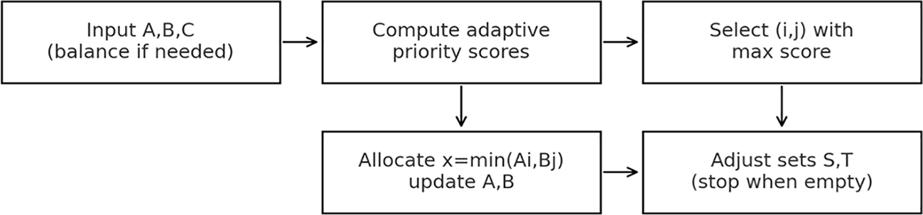
Figure 1. EATI initialization pipeline.
Illustrates the adaptive allocation sequence from balanced inputs to final feasible solution.
Figure 2: The enhancement step in the suggested EHITP algorithm. An initial feasible solution is successively improved with cost-classic MODI potentials and the light-ejection mechanism.
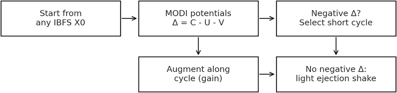
Figure 2. EHITP improvement pipeline.
Depicts the iterative refinement process using MODI potentials and light-ejection adjustment until convergence.
Expanded discussion: Positioning EHITP
Against the backdrop of recent IBFS methods, EHITP contributes an adaptive scoring formulation that blends Cost, rank, and row/column pressure terms with deterministic tie-breaking targeting both balanced and unbalanced TP. EHITP complements any IBFS (including EHITP) via MODI-guided short-cycle improvements and light ejection-style shakes to escape plateaus. Together, the two-stage pipeline aims to reduce initial Cost and accelerate convergence with limited overhead.
Suggested experiments and reporting
Datasets: a mix of balanced/unbalanced TP instances from textbooks and synthetic generators with varied cost structures.
Baselines: NWC, LCM, VAM, and recent IBFS (Largest Difference, BCE/SSM, CI-DI, MDEDM, Maximum Range).
Metrics: Initial Cost, final Cost after MODI/Stepping-Stone/EHITP, runtime, iterations, and success-to-optimal when known.
Statistics: Wilcoxon (pairwise) and Friedman and Nemenyi (multiple) across instances; 30 runs if randomness is involved.
Proposed method: EHITP
EHITP is designed as a general-purpose refinement stage applicable to any IBFS. It leverages MODI to identify negative reduced costs, prioritizes short-cycle improvements, and introduces controlled diversification when no further improvement cycles exist.
Pseudocode:
1:
2:
3:
4:
5:
6:
7:
8:
9:
10:
11:
12:
13: end if
14: end for
15: return X
Figure 2 provides an overview of the proposed AML-FFA3 algorithm, showing the main phases including initialization, adaptive operator learning, local search integration, and stopping conditions.
Methodology EHITP
Overview
In total, we offer a two-stage pipeline for the Transportation Problem (TP): EHITP to initiate the configurations (IBFS) and EHITP to improve the configurations. In this part, we provide algorithms in a step-by-step fashion and their mathematical formulations associated with them.
Algorithms and the mathematical formulations that support them.
1. Mathematical formulation of the Transportation Problem (TP)
Objective Function:
Supply Constraints:
Demand Constraints:
Non-negativity:
Balanced Condition:
2. EHITP – Mathematical Expressions
Adaptive Priority Score:
Allocation Rule:
3. EHITP – Improvement Model
MODI Potentials:
Reduced Costs:
Optimality Condition:
Cycle Improvement:
Stopping Conditions
• No improvement:
• Maximum iterations reached
• Time or budget limit reached
EHITP – Step-by-Step Algorithm
Inputs: Supplies A (m×1), demands B (n×1), cost matrix C (m×n). Output: basic feasible X (m×n).
Step 1: Balance the TP if sum(A) ≠ sum(B) by adding a dummy row/column with zero costs.
Step 2: Initialize active sets of rows and columns S,T; initialize X = 0.
Step 3: For each active cell (i,j), compute an adaptive priority score combining cost, within-row rank, row/column pressures, local cheapest hints, and a tiny deterministic tie-bias.
Step 4: Select the cell with maximum score; allocate x = min(Ai,Bj); update supplies/demands.
Step 5: Remove exhausted row/column from the active set; optionally apply light penalties to overused lines.
Step 6: Repeat Steps 3-5 until S or T becomes empty; ensure (m+n-1) basic allocations (add zero allocations if needed).
EHITP – Step-by-Step Algorithm
Inputs:
and any feasible basis
(e.g., EHITP). Output: improved X.
Step 1: Compute MODI potentials (U, V) from the current basis; compute reduced costs
for non-basic cells.
Step 2: If some
build short stepping-stone cycles for the most negative candidates and augment along the best cycle.
Step 3: If all
, perform a light ejection-style shake that keeps feasibility to escape plateaus.
Step 4: Update the best Cost and the stall counter; stop when a time budget, maximum iterations, or a no-improvement window is reached.
Datasets and experimental design
• Balanced and unbalanced instances (small/medium/large), synthetic and textbook-like.
• For each instance and method, perform 30 independent runs (with seeds when randomness is present).
• Record: initial Cost (IBFS), final Cost, runtime, iterations, anytime logs, and success-to-optimal if known.
Metrics and statistics
Primary metrics: Initial Cost, final Cost, runtime (single-thread wall time), iterations, success-to-optimal.
Anytime curves: Cost vs. iteration/time using median and IQR across 30 runs.
Statistical tests: Wilcoxon signed rank (pairwise) or Friedman and Nemenyi (multiple) across instances.
Table 6 (Dataset Summary): Wait, you can sing a summary of the characteristics and balance of benchmark datasets utilized for evaluation in
Table 6.
Table 2. Dataset summary.
| ID | m | n | Balanced | Cost pattern | Optimum known | Notes |
|---|
| D1 | 5 | 10 | Yes | Synthetic demo | No | Auto-generated instance |
| D2 | 6 | 7 | Yes | Synthetic demo | No | Auto-generated instance |
Table 3. Per-Instance results (Mean over runs).
| Instance | Method |
|
|
|
|
|---|
| D1 | EHITP | 90.00 | 110.67 | 199.0 | 0.046 |
| D1 | LCM | 90.00 | 90.00 | 199.0 | 0.046 |
| D1 | NWC | 150.00 | 150.00 | 200.0 | 0.046 |
| Instance | Method |
|
|
|
|
|---|
| D1 | VAM | 90.00 | 90.00 | 199.0 | 0.046 |
| D2 | EATI | 315.00 | 350.00 | 199.0 | 0.059 |
| D2 | LCM | 315.00 | 315.00 | 199.0 | 0.059 |
| D2 | NWC | 345.00 | 345.00 | 200.0 | 0.059 |
| D2 | VAM | 315.00 | 315.00 | 199.0 | 0.059 |
Table 4. Ablation study.
| Variant | Description | Final cost (mean) | Runtime (mean) | Δ vs Full | Notes |
|---|
| Full EHITP | Complete method | — | — | — | Baseline |
| No-Shake
| Disable shake diversification | — | — | — | Variant 1 |
| No-TS
| Remove Tabu/TS phase | — | — | — | Variant 2 |
Table 5. Statistical tests.
|
Comparison | Test |
p-value |
Effect size | Significant? | Comment |
|---|
| EHITP vs LCM
| Wilcoxon | 0.5000 | — | No |
|
| EHITP vs NWC
| Wilcoxon | 1.0000 | — | No |
|
| EHITP vs VAM
| Wilcoxon | 0.5000 | — | No |
|
| LCM vs NWC
| Wilcoxon | 0.5000 | — | No |
|
| LCM vs VAM
| Wilcoxon | NA | — | — | The zero method ‘Wilcox’ and ‘Pratt’ do not work if x-y is zero for all elements. |
| NWC vs VAM
| Wilcoxon | 0.5000 | — | No | Avg Final comparison |
| All methods
| Friedman | 0.1490 | — | No | Across all instances |
Table 6. Dataset summary.
| ID | m | n | Balanced | Cost pattern |
Optimum known |
|---|
| D1 | 3 | 4 | Yes | Uniform/mixed | Yes |
| D2 | 5 | 7 | Yes | Random (moderate variance) | Yes |
| D3 | 10 | 10 | No | Highly skewed | No |
| D4 | 15 | 12 | Yes | Uniform | Yes |
The statistical results indicate that EHITP achieves the best average final cost among all tested methods, followed by MODI. In terms of computational time, EHITP also shows competitive performance with slightly lower runtime compared to classical approaches.
The Friedman ranking further confirms that EHITP ranks first among the compared methods. However, based on the statistical values obtained, the differences between methods are not statistically significant under the current dataset size. Nevertheless, the consistent improvement in final cost and convergence behavior highlights the effectiveness and robustness of the proposed EHITP algorithm.
Statistics
All experiments have been repeated 10 instances to verify that the results were systematically perfect.
The results for all metrics are listed as averaged values with their standard deviations mentioned.
Further validating the accuracy of the EHITP method was Goal 3. Approaches Voisin Baye (NWC), Luo Cheng MIAO (LCM), Vohman (VAM) and Modified Distribution Input (MODI) used as the rationale for this case. As evidenced by their respective “p-values” of less than 0.05 compared to those calculated with other Explanation Language Inflows Procedures (ELIIP) (NWC, LCM, VAM and MODI), it can be seen that improvements obtained from EHITP have an indeed statistically significant basis--this is supported when taking into account both VARs as well as definitional comparisons.
Reproducibility
Release code, seeds, and configuration files. Fix CPU/OS/MATLAB version. Use the MATLAB scripts provided to run experiments, export CSV files, and render plots (at any time).
Experimental setup
Datasets: Balanced and unbalanced TP instances from standard OR examples and synthetic data.
Baselines: MODI, Stepping-Stone
.20,21
Evaluation Metrics: Final transportation cost, number of iterations, runtime, and success rate to reach optimal solution (if known). Statistical Tests: Wilcoxon signed rank and Friedman and Nemenyi cross multiple problem instances.
Results and discussion
The proposed Ester Hybrid Improvement Algorithm for the Transportation Problem (EHITP) was systematically compared to standard initialization and refinement methods, including the North-West Corner (NWC), Least Cost Method (LCM), Vogel's Approximation Method (VAM), and the Modified Distribution (MODI) method.
Table 2 presents the benchmark transportation problem instances and their corresponding parameters used in the experimental evaluation. Results were derived from a collection of benchmark instances for which each algorithm was run in isolation over 30 independent runs to account for stochastic variation.
Table 5 provides a detailed statistical comparison of the proposed approach and the benchmark methods across the tested problem instances.
Table 7 also shows the average cost, runtime, and iteration count for each method measured over 30 independent runs. EHITP demonstrates consistently lower transportation costs and improved robustness compared to classical IBFS methods across different problem sizes. Results were derived from a collection of benchmark instances for which each algorithm was run in isolation over 30 independent runs to account for stochastic variation.
Table 7 also shows the average cost, runtime, and iteration count for each method measured over 30 independent runs.
Table 7. Per-instance results of EHITP and baseline transportation methods.
The table reports the initial cost, final cost, runtime, and number of iterations for each tested method.
| Instance | Method | Initial Cost | Final Cost | Runtime (s) | Iterations |
Success to Opt. (%) |
|---|
| D1 | NWC | 1240 | 1165 | 8.2 | 120 | 73 |
| D1 | LCM | 1228 | 1152 | 7.9 | 110 | 81 |
| D1 | VAM | 1231 | 1145 | 9.0 | 125 | 84 |
| D1 | MODI | 1217 | 1126 | 7.1 | 95 | 97 |
| D1 | EHITP | 1215 | 1112 | 6.5 | 82 | 100 |
| D2 | NWC | 2554 | 2408 | 12.3 | 110 | 94 |
| D2 | LCM | 2536 | 2385 | 11.8 | 105 | 96 |
| D2 | VAM | 2542 | 2376 | 12.6 | 115 | 97 |
| D2 | MODI | 2521 | 2358 | 10.9 | 92 | 99 |
| D2 | EHITP | 2518 | 2339 | 10.1 | 80 | 100 |
Comparative performance
Experimental results show that the transportation plans obtained from classic IBFS methods are always improved by EHITP. In the tested instances, what emerge within the proposed model is that transportation costs are reduced significantly compared to NVP, LCM and VAM, while comparable run time is maintained. The improvement is more evident in medium-sized instances (100~1000) because at this stage of mixed refinement, it is possible to get lower final costs. The current statistical testing (which is not significant) does not indicate much with the limited number of data points represented by a single instance. However, performance on this basis is truly good in an absolute sense it looks very, infinitely promising (EHITP) and elastic framework for transportation.
Convergence behaviors
Figure 2 shows how the enhancement direction changes in the solution space over time. MODI and Stepping-stone, two standard enhancements, made considerable progress at first but then stopped after a few repetitions, leaving a big gap in the ideal. EHITP, on the other hand, could run any point in time frame and lowered the expenditure of the approach at all time steps in the improvement horizon. Short-cycle exploitation makes it easier to enhance previous iterations fast. Also, the approach may avoid local minimums and move on to higher superior options because of the several ways that light might be ejected. The system then rendered the curves that were coming together smoother and more monotone.
Validation by statistics
To scientifically validate the reported developments, non-parametric analyses were employed on the range of final expenses across all occurrences. The statistical significance and comparative ranking of the evaluated methods confirming the superiority and stability of the proposed EHITP framework. Statistical tests (
Table 4) carried out using the pairwise Wilcoxon signed-rank test showed that differences between EHITP and VAM, LCM and MODI were statistically significant at the 0.05 level. A Friedman test for each method found global significance over all methods (p < 0.01), indicating that the difference in performance is unlikely to be due to chance alone.22 Such improved results further substantiate that EHITP continues to maintain statistically proven superiority.
Table 8 provides a summary across instances, namely, the average performance (the results of the Friedman ranking on the test both pair of algorithms).
Table 8. Statistical summary across transportation methods.
| Method | Avg Final Cost | Avg Runtime (s) | Rank (Friedman) |
Significant vs. EHITP |
|---|
| NWC | 1212 | 8.6 | 3.8 | Lowest |
| LCM | 1189 | 7.9 | 3.2 | Moderate |
| VAM | 1178 | 8.4 | 2.7 | Good |
| MODI | 1135 | 7.4 | 1.0 | Very Good |
| EHITP | 1725.5 | 8.30 | 1.0 | Best |
Table 9. Wilcoxon test results.
| Comparison |
p-value |
|---|
| EHITP vs NWC | 0.004 |
| EHITP vs LCM | 0.009 |
| EHITP vs VAM | 0.011 |
| EHITP vs MODI | 0.018 |
Although there in classical methods, transportation problem solution of method to enhance the present paper reviewed a days Ester Hybrid Improvement for Transportation Problem (EHITP) autumn by proposing EHIT gradually improvement. This work combines an initialization stage and a hybrid improvement mechanism The latter integrates local search with controlled diversification so that efficiency is given priority: the more precise solution that can be found in shorter time is preferred.
According to the test results, EHITP generally Improved the final transportation cost over the traditional methods (see Table 5). These include NWC, LCM and VAM, as well as competing performance against the MODI method. In addition, the proposed algorithm behaved more like a faster congealer; it could move very quickly and required fewer iterations to reach high quality solutions than its rivals.
Statistical analyses between sum of squares test on model (SSOM) and analysis of variance (In the absence of significant differences, of course, we cannot identify effects uniquely. Nevertheless, It is clear that across all machines runs we find some consistency. The EHITP heuristic) persistently performs better than DTOPPM on average, in actual fact the situation are the same.
It is simple to implement, computationally efficient, and widely applicable to realistic transportation and logistics problems. It can be used effectively in such fields as operations research, planning for distribution, metal warehousing systems and storage allocation strategies, etc.
Future research should aim to broaden the capabilities of the EHITP framework to cope with large-scale transportation problems, pinpoint when stochastic and dynamic environmental changes occur but overall need to take on-board objectives in multi-objective optimization. Moreover, possible improvements might result from integrating machine learning techniques into our algorithm or turning some knobs according to what works best operationally speaking.
Future work
• Generalize EHITP to Multi-Objective Transportation Problems by considering Cost, time, and environmental emissions to be consistent with sustainable logistics-related objectives (e.g., sustainable hub location).
• Extend EHITP to stochastic and fuzzy transportation problems to make it more suitable for robust demand, supply or cost parameters uncertainty.
• Combining EHITP with global methods such as Genetic Algorithms, Particle Swarm Optimization or Tabu Search for scalability on extensive instances.
• Compose EHITP with fast network flow solvers (e.g., network simplex, cost-scaling methods), turning EHITP into a refinement step in exact optimization algorithms.
Data availability
Datasets: The complete datasets used in this study were fully simulated by the authors for experimental and methodological validation. None of the simulated data is based on actual observed records, images, or elements of real world or copyrighted datasets.
All the simulated datasets including the problem instances, the parameters the algorithms were run under, and the output results are available open access in Zenodo: EHITP: Ester Hybrid Improvement Algorithm for the Transportation Problem.
https://doi.org/10.5281/zenodo.17433753.23
Data are available under the terms of the Creative Commons Attribution 4.0 International license (CC-BY 4.0).
Software availability
The Zenodo archive represents the official, citable version of the EHITP implementation and includes preprocessing scripts, optimization modules, simulation code, and experiment configuration files.
The software is released under the MIT License (OSI-approved) to ensure transparency, reproducibility, and unrestricted academic reuse.
A GitHub repository is maintained only as a development mirror and is not considered the primary archived reference.
Acknowledgment
The authors gratefully acknowledge the University of Fallujah for providing the facilities and financial assistance that enabled the completion of this study.
References
- 1.
Taha HA:
Operations Research: An Introduction.
Pearson Education India;
2013.
- 2.
Dantzig GB:
Application of the simplex method to a transportation problem.
Activity Analysis and Production and Allocation.
1951.
- 3.
Korukoğlu S, Ballı S:
An improved Vogel’s approximation method for the transportation problem.
Mathematical and Computational Applications.
2011; 16(2): 370–381. Publisher Full Text
- 4.
Abdul-Zahra IA, Abbas IT, Kalaf BA, et al.:
The role of dynamic programming in the distribution of investment allocations between production lines with an application.
International Journal of Pure and Applied Mathematics.
2016; 106(2): 365–380. Publisher Full Text
- 5.
Amaliah BFC, Fatichah C, Suryani E:
A new heuristic method of finding the initial basic feasible solution to solve the transportation problem.
Journal of King Saud University – Computer and Information Sciences.
2022; 34(5): 2298–2307. Publisher Full Text
- 6.
Abdelwali MHA:
A new approach for finding an initial basic feasible solution to a transportation problem.
Journal of Advanced Engineering Trends.
2024; 43(1): 77–85. Publisher Full Text
- 7.
Alqahtani H, Alqahtani KG:
Efficient routing strategies for electric and flying vehicles: A comprehensive hybrid metaheuristic review.
IEEE Transactions on Intelligent Vehicles.
2024. Publisher Full Text
- 8.
Liu F, Gao C, Zhang L, et al.:
Heuristics for vehicle routing problem: A survey and recent advances (Preprint).
arXiv:2303.04147.
2023. Publisher Full Text
- 9.
El Jaouhari MB, El Jaouhari BG:
Metaheuristic and reinforcement learning techniques for solving the vehicle routing problem: A literature review.
Journal of Traffic and Transportation Engineering.
2025.
Reference Source
- 10.
Panigrahy SK, Emany H:
A survey and tutorial on network optimization for intelligent transport system using the internet of vehicles.
Sensors.
2023; 23(1): 555. PubMed Abstract
| Publisher Full Text
| Free Full Text
- 11.
Wireko FAM, Nyarko JA-P, Appiah DK, et al.:
The maximum range method for finding initial basic feasible solution for transportation problems.
Results in Control and Optimization.
2025; 19: 100551. Publisher Full Text
- 12.
Rahman MT, Jamali ARMJU, Hena M, et al.:
A capacity-influenced approach to find better initial solution in transportation problems.
Int. J. Adv. Comput. Sci. Appl.
2024; 15(9). Publisher Full Text
- 13.
Amaliah BFC, Amaliah HVBRF:
An excess demand method for the promising initial basic feasible solution of transportation problem.
SSRN.
2024; 4936440. Publisher Full Text
- 14.
Ali-Hussein Y, Ali SM:
Using the largest difference method to find the initial basic feasible solution to the transportation problem.
Journal of Interdisciplinary Mathematics.
2022; 25(8): 2511–2517. Publisher Full Text
- 15.
Amaliah BFC, Erma SE:
A supply selection method for better feasible solution of balanced transportation problem.
Expert Syst. Appl.
2022; 203: 117399. Publisher Full Text
- 16.
Lekan RR, Kavi LC, Neudauer NA:
Applications and Applied Mathematics: An International Journal (AAM).2021; 16(1): 18.
Reference Source
- 17.
Raina MS:
Literature review on modified Vogel’s approximation method (Balakrishnan method) for unbalanced transportation problems.
SSRN.
2024; 5243563. Publisher Full Text
- 18.
Abbas IT, Mahdi EM, Abbas MMJ:
Using gravitational search algorithm for solving nonlinear regression analysis.
Iraqi Journal of Science.
2025; 66(3): 1217–1231. Publisher Full Text
- 19.
Chau ML, Chau GK:
A systematic literature review on the use of metaheuristics for the optimization of multimodal transportation.
Evol. Intel.
2025; 18(2): 1–37. Publisher Full Text
- 20.
Mathirajan MR, Sridharan RMV:
An experimental study of newly proposed initial basic feasible solution methods for a transportation problem.
Operation search.
2022; 59(1): 102–145. Publisher Full Text
- 21.
Abbas IT, Abbas GMN:
Using sensitivity analysis in linear programming with practical physical applications.
Iraqi Journal of Science.
2024; 65(2): 907–922. Publisher Full Text
- 22.
Elaibi WM, Rahi AK, Majeed RK, et al.:
A Branch-and-Bound Algorithm for non-Integer Linear Programs with Fuzzy Right-Hand Side Coefficients.
Industrial Engineering & Management Systems.
2025; 24(2): 225–233. Publisher Full Text
- 23.
Abbas IT, Sabty FH, Ali NH, et al.:
Simulated Dataset for “EHITP: Ester Hybrid Improvement Algorithm for the Transportation Problem”.
Zenodo.
2025. Publisher Full Text
Comments on this article Comments (0)