Keywords
Two-dimensional turbulence, Negative absolute temperature, Point vortex system, Linear response theory, Mean-fileld theory
This article is included in the Japan Institutional Gateway gateway.
Two-dimensional turbulence, Negative absolute temperature, Point vortex system, Linear response theory, Mean-fileld theory
Main topic of this paper is a vortex dynamics in a two-dimensional (2D) system.
We analytically investigate the formation mechanism of a depleted vorticity region around a strong vortex injected into a uniform background vorticity field. A delta-function-type strong vortex is impulsively injected as a perturbation into an equilibrium state of uniformly distributed vorticity. In response to the injected impulse vortex, a region of depleted vorticity is formed in the vicinity of the impulse vortex. This phenomenon was discovered in two-dimensional vortex experiments using pure electron plasmas. An overview of these experiments is presented later. In this paper, we provide an analytical explanation for the formation of the depleted vorticity region using linear response theory and mean-field approximation for two-dimensional point vortex systems.
In three-dimensional turbulence, the Richardson cascade is a well-known phenomenon in which system energy is transported from large scales to small scales and is ultimately dissipated through viscous effects.1,2 In contrast, two-dimensional turbulence is characterized by the inverse cascade, which differs from three-dimensional turbulence.3,4 In the inverse cascade, energy is transported from small scales to large scales, leading to the formation of large-scale vortices. Furthermore, when numerous small-scale vortices aggregate, they form highly organized structures resembling a crystalline lattice. This phenomenon is sometimes referred to as self-organization.
To observe structure formation in two-dimensional turbulence, it is necessary to track the time evolution over long periods, which requires inviscid or approximately high Reynolds number flow experiments. A pure electron plasma system is well-suited for this purpose.5 Let us consider electrons confined in a vacuum chamber with a strong axial magnetic field. The 2D motion of the electrons perpendicular to the axial magnetic field is described by the 2D incompressible, inviscid Euler equation.6–8 The electron number density and the self-induced electrostatic potential are proportional to the vorticity and the stream function, respectively. Two groups at Kyoto University and at University of California, San Diego have independently reported pure electron plasma experimental results on two-dimensional turbulence and structure formation.9–14
Onsager proposed the concept of negative absolute temperature as a key to understanding the inverse cascade phenomenon.15–17 The state with corresponds to a phenomenon in which the statistically defined (inverse) temperature becomes negative, where is the entropy and is the (internal) energy. The entropy and the number of accessible states of the system are related by where is the Boltzmann constant. Therefore, although unusual for conventional systems, negative absolute temperature can occur in systems where the number of accessible states decreases as the energy increases. Point vortex systems are known as representative examples of systems that can exhibit negative absolute temperature states.
The point vortex system serves as a tool for representing two-dimensional flows. In this system, the vorticity field is represented by a collection of point vortices discretized as delta functions (described later). As same-sign point vortices coalesce into a single location, the degrees of freedom regarding their configuration decrease while the energy increases. That is, since the number of accessible states decreases with increasing energy, this system can exhibit states with . It was numerically demonstrated by Joyce et al. that point vortices confined in a rectangular domain with periodic boundary conditions form a clustered state.18,19 Using large-scale simulations with special-purpose supercomputer MDGRAPE-2, the negative temperature properties observed in point vortex systems confined within a circular boundary was examined by Yatsuyanagi et al.20
The point vortex system can serve as a powerful tool not only for numerical simulations but also for theoretical analysis.21,22 In experiments conducted by the Kyoto University group, the formation of a depleted region around a strong vortex was observed, but the mechanism behind this phenomenon remained unclear for a long time.23 In the present study, to describe the phenomenon, we derive the two-body correlation function analytically, employing the linear response theory and the mean-field approximation for the point vortex system. The linear response is the response of a system in equilibrium to a perturbation imposed by an external field, where the perturbation is weak enough not to destroy the equilibrium state. In a discrete particle system, the mean field is defined as the continuous particle distribution function that emerges in the infinite particle limit. This approach is referred to as the mean-field approximation. Injecting a delta-function-type strong vortex impulsively as a perturbation into an equilibrium state of uniformly distributed vorticity, we evaluate the response as the two-body correlation function. The obtained function indicates that a region exhibiting a negative response to the impulse input emerges.
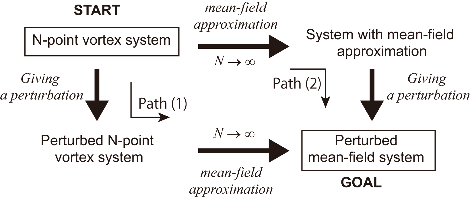
Organization of this paper is as follows: In Sec. II, we first introduce the two-dimensional fluid experiments using pure electron plasma and the experimental result that motivated this study (Sec. II A). Subsequently, we define the two-dimensional point vortex system used as an analytical tool (Sec. II B), and present the results calculated via the route of Path (1) (Sec. II C) and the route of Path (2) (Sec. II D) in Figure 1. Then, by imposing the condition that the results obtained from the above two routes should be equal, we derive the equation that the two-body correlation function must satisfy (Sec. II E). In Section III, we obtain the homogeneous solution (Sec. III A 1) and the special solution (Sec. III A 2) of the equation derived in Sec. II E. Finally, in Section IV, we examine the conditions that the two-body correlation function must satisfy in a system with circular boundaries, and present the explicit solution of the two-body correlation function.
In this section, we present the experimental results obtained with pure electron plasmas. Electrons are confined in a cylindrical vacuum chamber radially by a strong magnetic field along the axis of the chamber and axially by the negatively biased electrostatic potentials at both ends. When the electrostatic potential at one end of the chamber is turned off, electrons are released along the axis and strike a phosphor screen positioned perpendicular to the magnetic field. The resulting luminosity distribution is recorded by a Charge Coupled Device (CCD) camera. As this measurement is destructive, the experiment requires high reproducibility. Details of the experimental configuration are found in Refs. 9, 24, 25. The electron motion perpendicular to the magnetic field is described by the 2D Euler equation,6,7 in which the electron density is proportional to the vorticity.
The time evolution of the electron distribution is shown in Figure 2. The brightness in this figure is proportional to the electron density, i.e., the vorticity. In this experiment, we first established an uniform equilibrium electron distribution as the background vortex, and then injected an electron population with a density higher than that of the background. A region where electrons are concentrated at a density higher than the background distribution is referred to as a clump. In this case, the vorticity inside the clump is about 180 times higher than that of the background.
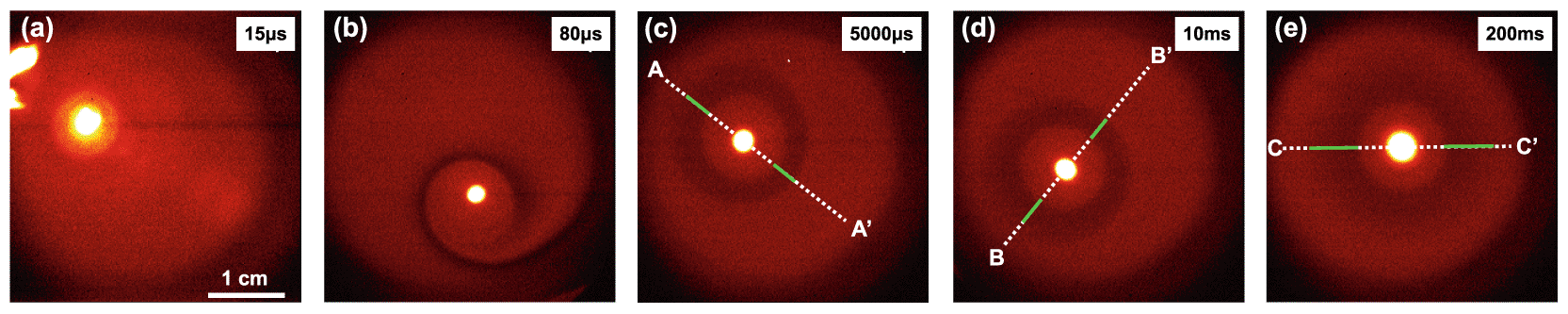
Shown are snapshots of the electron density at (a) 15 μs, (b) 80 μs, (c) 5 ms, (d) 10 ms, and (e) 200 ms.
The clump migrates toward the center of the background vortex through the interaction of its self-induced swirling flow with the background vortex. As the clump moves, it entrains low-vorticity regions from outside the background vortex, creating a ring hole of reduced vorticity around it. We will explain the mechanism of ring hole formation using the two-point correlation function of vorticity.
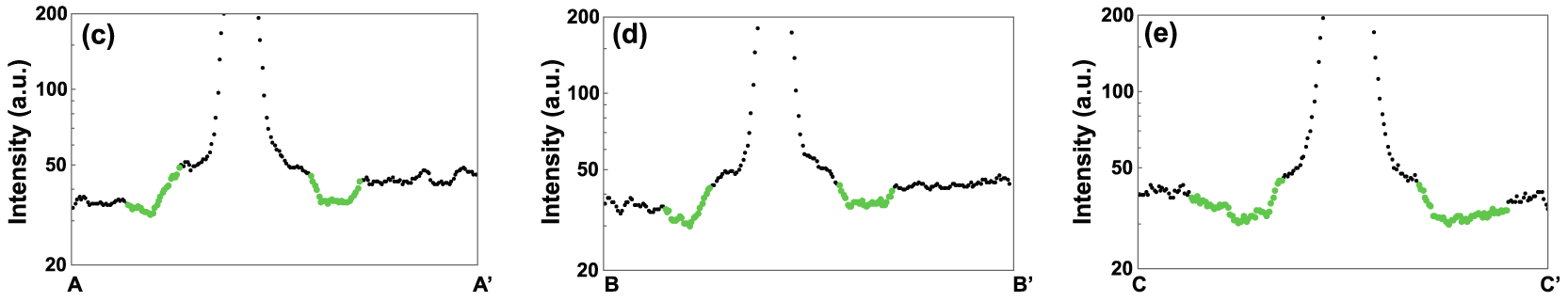
The density depression around the clump is depicted in Figure 3. Figure 3 plots the density profiles along lines A-A’, B-B’, and C-C’ shown in Figures 2 (c), (d), and (e), respectively. Points A, A’, B, B’, C, and C’ are located in the background vortex, and regions with density lower than the background are highlighted in green. The green regions indicate areas exhibiting negative correlation.
In this section, we define a two-dimensional (2D) system considered and introduce prerequisite for calculating the explicit formula of a two-body correlation function for the system.
1. 2D point vortex system
Let us consider a collection of singular point vortices, which defines a 2D vorticity field :
The position vector of the -th point vortex is given by . Each vortex has a constant circulation . The notation is the 2D Dirac delta function. A quantity depending on the positions of the singular point vortices is indicated by . We call a variable with as the microscopic one. The total circulation is assumed to be finite and constant, namely
A stream function is defined by
The stream function (3) and the vorticity (1) are related by the Poisson equation
2. Hamiltonian
The following integral corresponding to energy of the system diverges at
A quantity without an external perturbation (see below) is indicated by the suffix .
3. External perturbation
A macroscopic stream function without is introduced as an external arbitrary perturbation, which defines a microsopic stream function
The quantity denotes Hamiltonian with an external perturbation .
For convenience, we introduce a suffix where the asterisk matchs either 0 or . In an equation which contais two or more asterisks, all the asteriscs are unifiedly replaced by either 0 or .
4. Partition function
A partition function is defined by
According to the assumption (2), the inverse temperature is chosen to be
Under the above condition and the definition (7), the dependence of Hamiltonian on is estimated as
This shows the free energy is well-defined regardless of the magnitude of .
5. Canonical average
The canonical average converts a microscopic quantity into a macroscopic one. There are two kinds of canonical average, and . The notation represents the average with , and the notation represents the average with , namely,
6. Fluctuation
The fluctuation is defined by the subtraction of the canonical averaged quantity from the microscopic one which depends on the particle position :
7. One-body distribution function
The one-body distribution function is defined by
Due to the symmetry of under the permutation of the -th and the -th particles, it satisfies
8. Two-body distribution function
The two-body distribution function is defined by
Note that is not defined on as is not defined on .
The goal of this section is to derive a linear response formula for the -point vortex system to a fluctuation (path (1) in Figure 1).
1. Linear response formula
As a general procedure, we calculate a functional derivative two times to obtain a correlation of the fluctuation .26 The functional derivative is carried out by introducing an arbitrary external perturbation ( ) and differentiating with respect to twice.
We represent the integrand as the functional delivative
Similarly, the second-order delivative is obtained:
In the limit , i.e., , Eq. (25) is written as
As an important result in relation to Eq. (26), a response to an external perturbation defined by
It should be noted that Eq. (28) has the same form as the general linear-response formulae.26
2. Two-body correlation function
The two-body correlation funcntion in a thermal equilibrium state is defined by
The aim of the present analysis is to determine in the limit of vanishing external perturbation. Characteristics of the correlation function for long-range interacting particle system was discussed by Ornstein and Zernike.27,28 A basic idea introduced by them is to split an effect of the correlation function into a self-correlation and a mutual correlation, which is called Ornstein-Zernike formula. For the point vortex system, the formula is rewritten as
The first term of Eq. (30) in the right hand side corresponds to the self-correlation and the second term the mutual correlation. Substituting Eq. (30) into (28), we obtain the formula for the linear response in the point vortex system.
This formula is the main conclusion, representing the linear response of the system derived from the two-body correlation function.
Mean-field theory is an approximation technique in which terms proportional to square of the fluctuation are neglected. The goal of this section is to derive a linear response formula for the mean-field approximated point vortex system.
1. Hamiltonian in the mean-field approximation
In the mean-field theory, physical quantities are represented by the sum of the mean-filed quantity and a fluctuation. There are two possible representations, with (suffix “e”) and without (suffix “0”) the external field:
Note that the second term in the right hand side of Eq. (32) depends on the particle coordinate . Thus, the term has the hat .
The Hamiltonians and in the mean-filed approximation are given by
2. Partition function
The partition functions and are defined by
3. Free energy
The free energy and are defined by
4. Thermal equilibrium state
A thermal equilibrium state is defined by minimization of the free energy. The condition is given by
Upon explicit calculation, we obtain:
By operating on Eq. (43), the following formula is obtained.
Similarly, the formula without a perturbation is also obtained.
The solution to this Poisson equation is derived here, as it will be required in subsequent sections. Substituting
The solution to Eq. (47) in was discussed by Chen and Li.29 The solution to Eq. (47) exists only when and the solution is given by
Thus, the solution of Eq. (45) is given by the following formulae and those of the parallel translation:
5. Response in the mean-field theory
The responses in the mean-field theory is defined by
Using Eqs. (53) and (54), Eq. (44) is linearlized.
Equation (55) is the final formula of the response to the external field in the mean-field theory.
We have otaintained two formulae for the response, Eq. (31) and Eq. (55). We assume that , in Eq. (31) coincde with , in Eq. (55), respectively:
Applying the operator to Eq. (56), where denotes the Laplacian with respect to , we obtain
Substituting Eq. (55) into Eq. (58), the following equation is obtained.
As is an arbitrary function, Eq. (59) is reduced to
In the next section, we will solve Eq. (60) and obtain an explicit formula for .
1. Homogeneous solution
Now, we are ready to solve Eq. (60). At first, we will obtain the homogeneous solution to Eq. (60), namely, the solution to
Here, we have used the following relation with fixed .
Equation (62) is reduced to
2. Special solution
In the next we will obtain a special solution to Eq. (60) with .
Consider Eq. (47) with a perturbation whose solution is denoted by :
The limit of the partial derivative of Eq. (66) with respect to at fixed is given by
The above equation is reduced to the following form:
By employing the practical form of
We conclude that the complete solution to Eq. (60) is given by the combination of the homogeneous solution (65) and the imhomogeneous solution (74), namely,
In general, the correlation function satisfies the following two conditions:
To derive the correlation function, we have used an mean field approximation. Mean-field approximation generally fails in systems with strong correlations. That is, we consider that the first condition is already fulfilled.
Let us examine the second condition. One-body distribution function in an equilibirium state is given by Eq. (52)
Integrating Eq. (75) in , we obtain
Perform a change of variables in the integral
Perform a change of variables in the integral
We find that the -dependence does not remain in the integral result. To overcome this difficulty, cutoff radius is introduced. According to this change, we replace the integral domain with and search the value of which satisfies
Returning to Eq. (85), we re-evaluate the above integral.
Thus, we obtain satisfying condition (87).
By introducing a conditional probability that assumes the presence of a particle at the origin as the source of perturbation, the two-body distribution function effectively reduces to a one-body distribution function. Applying the above condition to Eq. (29) yields
Among the terms in the above expression, corresponds to the linear response part, where is defined in Eq. (75). Figure 4 shows a plot of this function. As anticipated, a region with negative correlation forms in the vicinity of the origin in response to the perturbation imposed at the origin. It should be noted that since the term is proportional to , the magnitute of the response is small compared to the leading-order term of 1. Thus, although we successfully obtained the two-body correlation function analytically, its effect is small and only qualitative agreement is achieved. In other words, additional quantitative analysis may be required to refine the explanation for the formation of the depleted region observed in the experiments.
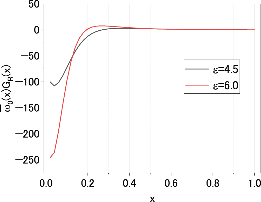
The value of R is 1.0. As anticipated, a region with negative correlation forms in the vicinity of the origin in response to the perturbation imposed at the origin.
Further efforts are necessary to quantitatively explain the experimental results. The two-body correlation function that we analytically derived in this work remains within the linear response regime and does not address the longer-time dynamics. Since analytical treatment of the time evolution of the system is expected to be difficult, we are preparing large-scale numerical simulations using a supercomputer equipped with the latest PEZY-SC4s processor, a platform that one of the authors (Y.Y.) has been utilizing. Numerical simulations will enable us to capture the detailed particle transport behavior, allowing us to investigate in detail aspects such as the destination of particles during the formation of the depleted region.
| Views | Downloads | |
|---|---|---|
| F1000Research | - | - |
|
PubMed Central
Data from PMC are received and updated monthly.
|
- | - |
Provide sufficient details of any financial or non-financial competing interests to enable users to assess whether your comments might lead a reasonable person to question your impartiality. Consider the following examples, but note that this is not an exhaustive list:
Sign up for content alerts and receive a weekly or monthly email with all newly published articles
Already registered? Sign in
The email address should be the one you originally registered with F1000.
You registered with F1000 via Google, so we cannot reset your password.
To sign in, please click here.
If you still need help with your Google account password, please click here.
You registered with F1000 via Facebook, so we cannot reset your password.
To sign in, please click here.
If you still need help with your Facebook account password, please click here.
If your email address is registered with us, we will email you instructions to reset your password.
If you think you should have received this email but it has not arrived, please check your spam filters and/or contact for further assistance.
Comments on this article Comments (0)