Keywords
deep learning; stock price forecasting; minute-level data; Optuna-based denoising; developing markets; Sharpe ratio; LSTM for forecasting; Adaptive Market Hypothesis.
deep learning; stock price forecasting; minute-level data; Optuna-based denoising; developing markets; Sharpe ratio; LSTM for forecasting; Adaptive Market Hypothesis.
Global investors traditionally prefer mature, liquid, and information-efficient developed equity markets such as the US, Japan, and Singapore. In contrast, developing markets (India, Brazil, Malaysia, etc.) often do not find their way into global portfolios, as they are frequently overlooked due to volatility, currency risks, and perceived informational inefficiencies.71–73 This “flight to safety” persists despite the Adaptive Market Hypothesis, which suggests that some of the very inefficiencies and volatility clustering cited as risks in developing markets may create exploitable short-term patterns for sophisticated traders.1,2
The challenge of exploiting these patterns is magnified at high frequencies. Minute-level stock data is inherently non-stationary and plagued by a low signal-to-noise ratio due to microstructure effects, such as bid-ask bounces. These issues are acute in developing economies, which tend to have thinner liquidity and external shocks play a bigger role; this can result in larger forecasting errors. Yet, sophisticated architectures of deep learning algorithms (from Long Short-Term Memory (LSTM) networks to Transformers and CNN-LSTM hybrid networks) do a great job of capturing nonlinear patterns in such noisy data. By exploiting mechanisms such as gating units (in LSTMs/GRUs) for long-term dependencies, dilated convolutions (in TCNs) for extended receptive regions and self-attention (in Transformers), these technologies have the potential to turn the perceived risks of insufficiently efficient environments into a trustworthy source of alpha.3,4,74
This research addresses an important gap in the literature: no other study has systematically compared whether deep learning, when applied to denoised minute-level data, produces better risk-adjusted intraday returns in developing versus developed markets using an identical methodological pipeline. We provide the first controlled analysis across matched large-cap stocks, isolating pure price signals (excluding traditional technical indicators) and constructing distinct long (buy) and short (sell) portfolios to empirically challenge the persistent investor bias toward developed markets.
To ensure a rigorous comparison, our pipeline employs Optuna-optimised denoising (incorporating wavelet transforms, autoencoders, and Kalman filters) to filter microstructure noise before training models with walk-forward validation. We specifically chose India, Brazil, Malaysia as developing markets due to their balanced liquidity and stability evidenced by the strong inflows of FDI (e.g., US$81.04 billion for India during FY2024–25; ~US$84.1 billion for Brazil through Nov 2025; strong inflows for Malaysia) and stable projections of GDP growth (e.g., ~6.6% for India, ~2.5% for Brazil, ~4.4% for Malaysia).3–6,9 We deliberately omitted other developing regions (e.g., sub-Saharan Africa - e.g. South Africa; smaller Asian economies - e.g., the Philippines) because the literature shows that they have much higher risks (e.g., political instability and low FDI inflows; e.g., US$8.9 billion for the Philippines in 2024) and this could be a source of bias in drawing comparisons (e.g.,7,8). This selection enables fair, high-frequency comparisons with developed economies.
In sum, this study shows that Deep Learning based on denoised data at the min level can leverage inefficiencies in developing markets to deliver superior risk-adjusted returns at the intraday level vis-a-vis developed markets, challenging the conventional bias among investors that under-utilises opportunities to generate alpha. By exploiting the natural volatility of these markets with sophisticated computer methods, the results highlight the possibility of liquid emerging large-cap stocks as useful sources of diversification and enhanced returns within global portfolios. This work not only fills the gap between theoretical market inefficiencies and practical trading strategies but also offers a replicable framework for geo traders to exploit short-term opportunities in less efficient environments.
To address the prevailing investor bias and validate the efficacy of deep learning in these regions, this study poses the following research objectives:
a) To investigate the behavioral disparity in capital allocation: We aim to understand why investors prioritize developed nations despite the theoretical high-growth potential and exploitable inefficiencies in developing ones. Specifically, we ask: Why do investors considering investments in developed nations not also consider investments in developing ones?
b) To evaluate the risk-return trade-off via computational methods: We identify the development markets that have the same or better risk-return trade-offs to the intraday trading when using advanced denoising and deep learning. We ask the following question: Are the developing countries equal or better off in terms of risk-return trade-offs due to current market conditions, available computational powers and favorable macroeconomic environment?
c) To assess the viability of liquid developing markets: We examine whether statistically significant markets, such as India, Brazil, and Malaysia, provide viable trading opportunities and diversification benefits comparable to major developed economies. This addresses the question: Can investors invest in statistically significant markets like India, Brazil, and Malaysia, as well as similar, statistically stable, and opportune equity markets, and expect comparable returns or trading opportunities?
These objectives highlight the importance of empirically analysing the interaction between market microstructure and deep learning, which is the main motivation for this work.
Motivated by the juxtaposition of the high growth potential of developing markets with their underrepresentation in global portfolios, this work aims to empirically challenge the “flight to safety” bias. Our main contribution is to show that it is possible to systematically extract alpha from these environments using deep learning, and to present solid evidence for the impact of computational advances in reducing the volatility of developing markets and converting it into actionable, high-quality returns.3,10 Furthermore, by providing a replicable framework for denoising high-frequency data, this research offers a practical methodology for institutional investors to cross the boundary of complex data challenges in developing economies and effectively bridge the gap between theoretical market inefficiencies and trading utility in the real world.
Our unique value is creating opportunities for intraday trading in developing economies. By applying market-standard statistical methods, we validate that investors can participate in the equity markets of developing economies to secure daily trading returns and effectively expand the global investment horizon beyond traditional developed markets.
The disparate performance of developed and developing equity markets is one of the oldest and most basic theories of economics. At the centre of this distinction is the idea of the Equity Risk Premium (ERP) - the excess return over the risk-free rate that investors expect to be paid to compensate them for the higher level of systematic risk they are taking.5,11–13 In emerging markets (e.g., USA, Japan, Singapore) the risk will be of a higher nature due to several elements such as political instability, currency fluctuation, and liquidity.5,11–13 In a more technical manner, while developed markets are characterised by mature institutions and fast information diffusion, developing economies often have persistent inefficiencies and are acutely susceptible to external shocks.13–16 A prominent study published confirmed this delusion by showing that emerging markets exhibit much higher volatility clustering during global crises than their developed counterparts.
Recent publications further highlight these dynamics. For instance, a recent causality investigation of stock prices and macroeconomic indicators in the Indian stock market reveals a tight relationship between volatility in developing economies and macroeconomics, which, in turn, influences asset pricing.17 Similarly, research on behavioural biases in the Indian market shows that psychological factors, for instance, overconfidence and disposition effects, amplify under-allocation to developing markets.3,18 Furthermore, recent work on cointegration in the Indian stock market focuses on spillover effects, in line with the idea that the volatility of developing markets can spread but can also provide unique opportunities for diversification.19
However, the Adaptive Market Hypothesis (AMH) challenges the traditional Efficient Market Hypothesis (EMH) by positing that market efficiency is a dynamic process rather than an absolute state1 further suggests that inefficiencies, e.g., time delays in price discovery and volatility clustering, are not only risks but also opportunities for exploitable patterns. This view has empirical support, suggesting that in developing markets, weak-form efficiency is very rare and, as a result, arbitrage opportunities still exist and can be exploited with sophisticated computational models.20,21 This framework implies that behavioural biases may cause investors to under-allocate capital to developing markets, where informational inefficiencies could be exploited to generate alpha.2,18
Traditional econometric models (e.g., ARIMA, GARCH) have been the standard tools for financial prediction.22,58 have extensively detailed the use of ARIMA models for stock trend forecasting. However, these linear models can struggle to account for the complex nonlinearities and regime shifts in high-frequency financial data.23 Consequently, Deep Learning (DL) has emerged as a great alternative, with its adaptive feature learning and its superior generalization on out-of-sample data.
A recent bibliometric review on artificial intelligence and finance, published by,24 charts this evolution, showing a proliferation of neural network applications for predictive modelling and volatility analysis after 2010. This corresponds to our move towards DL for processing noisy & high frequency data for time series forecasting.
A. Sequence Models (LSTM, Bi-LSTM, GRU): Long Short-Term Memory (LSTM) networks established a benchmark for financial time series by effectively managing long-term dependencies25 demonstrated that LSTMs-based predictions achieved, and the portfolio generated daily returns of 0.46% and a Sharpe ratio of 5.8 (before transaction costs) on S&P 500 data, significantly outperforming memory-free methods, such as random forests. Subsequent research has led to the optimization of such architectures3: showed that Bidirectional LSTMs (Bi-LSTM) can be used to increase context awareness in volatile series, with up to 70% directional accuracy26; showed that Gated Recurrent Units (GRU) give similar performance with converging times of 20–30% faster than Bi-LSTMs.
B. Convolutional and Attention-Based Models: To obviate the sequential processing limitations on recurrent architectures, Temporal Convolutional Networks or TCNs were introduced as a dilated convolution technology to solve the long runtime problems of long-range modelling in parallelizable computations, and could be superior to standard LSTMs in high-frequency tasks.27,28 Furthermore, Transformers can use a self-attention mechanism to capture global dependencies across long-term horizons, achieving the lowest Root Mean Square Error (RMSE) in intraday regimes.29,30
C. Hybrid Architectures: Recent surveys name hybrid models, e.g. CNN-LSTM or Conv1D-LSTM, as state-of-the-art. Zhang et al. (2019) showed that CNNs are particularly useful for extracting local features from high-frequency microstructure data (e.g., limit order books). These architectures mix convolutional layers for feature extraction and recurrent layers for sequence modelling, being top-ranked in empirical surveys for accuracy and being less prone to overfitting.23,31 However, issues such as overfitting in volatile regimes persist, which basically calls for a good validation technique.
Minute-level financial data is almost always noisy, with microstructure effects, such as bid-ask bounces, that obscure fundamental price trends. To perform effective forecasting, rigorous denoising is necessary to improve the Signal-to-Noise Ratio (SNR).
A. Denoising Techniques: Wavelet transforms are widely used to decompose signals and remove high-frequency irregularities.32,33 Furthermore,34 provided influential evidence that integrating stacked autoencoders (SAEs) with LSTMs significantly improves predictive performance by reconstructing clean price signals via neural compression.35 While effective, these methods require careful parameter tuning to avoid signal loss.
B. Optimization with Optuna: A major improvement to pipelines today is the automated tuning of denoising parameters. Optuna, which uses a Tree-structured Parzen Estimator (TPE), optimises hyperparameters (such as wavelet thresholds and latent dimensions) 30%–50% faster than grid search.36 This guarantees reproducible and robust noise reduction, resulting in clearer signals for subsequent deep learning models. Critically, empirical review studies indicate that denoising optimisation strategies can reduce RMSE by 15–30% in noisy financial series, although the effectiveness of optimal denoising strategies can vary across market conditions.37
Overfitting is a major issue for the prediction of financial time series, as models can learn noise instead of generalizable patterns - a particular danger with volatile developing markets.10,23 This is especially true of deep learning models for regime shifts. To mitigate this, it is important to implement rigorous validation protocols.
This research follows the standards promoted by,38 using Walk-Forward Validation rather than traditional k-fold cross-validation.75 This way, temporal order is preserved without look-ahead bias, and the model is tested on “future” data that does not exist or that it had never seen during training.39 Combined with regularisation techniques inherent in modern architectures (e.g., dropout layers in LSTMs), this validation strategy ensures that the alpha generated is robust and not merely an artefact of overfitting.
To ensure a fair and representative comparison across markets, stock selection must account for the varying market structures40 demonstrated that K-means clustering based on market capitalisation and beta effectively groups stocks by risk-return profiles, improving prediction accuracy by 10–20% compared to random selection.
For portfolio construction and validation, this study adheres to the rigorous standards advocated by,38 employing Walk-Forward Validation rather than traditional k-fold cross-validation to preserve temporal order and prevent look-ahead bias. We employ Inverse Volatility Weighting for portfolio allocation. In high-frequency regimes, estimating stable covariance matrices is notoriously unstable; inverse volatility weighting prioritises risk control, dynamically allocating capital to lower-volatility assets to minimise drawdowns—a critical feature for short-term strategies.41,42 Compared to alternatives such as Mean-Variance Optimisation, this method offers greater robustness in volatile, developing markets, though it may underperform in low-volatility environments.
Despite extensive literature on financial forecasting (e.g.,76), significant gaps remain in the systematic comparison of developed and developing markets using high-frequency data.
Table 1 summarizes the current literature on financial forecasting, pointing out the methodological voids in the literature and indicating how the current paper addresses them by Optuna-tuned denoising pipelines.
The proposed forecasting and portfolio construction pipeline comprises the following stages, as described by a lucid chart below:
The stepwise analysis is explained below:
a) Data Collection: The minute price data from 6 countries (3 developed and 3 developing countries) for the last 30 days are collected.
b) Price denoising & signal generation: Selected companies are then fed into the denoising process to generate predictive pattern price signals, which could further be trained in DL (Deep Learning) models for price forecasting accuracy.
c) Prediction Model: The denoised price signals are then fed into various DL methods with Optuna-defined hyperparameter optimisation that assures the best possible training accuracy for future signals.
d) Validation of Price Dataset: We finally employ a selected set of future price datasets, which are tested in segments of 10 batches for 30 prices in each batch, for error-based walk forward prediction and finally correction of prediction based on corrected features.
e) Finally, the predicted prices with the highest adjusted R2 scores and low overfitting scores are selected for accuracy testing, which are used by price timestamp in portfolio creation for generating the best possible portfolio.
The overall research process involves support of the lowest possible volatility by two sequential steps:
1. The Denoising process, it reduces high-frequency signals through Optuna-based optimisation.
2. By DL based prediction process, the method ensures that Optuna-based hyperparameter optimisation only trains on low-frequency signals, which assures the best possible correction through walk-forward validation.
The research also assures that after successful price prediction confirmation of the predicted price signals, which are successful by directional accuracy, the predicted timestamp with the highest and lowest price is used for real prices for portfolio development, and both the increasing price options are used for buy and the decreasing price options are used for sell portfolio. Furthermore, an inverse price volatility-based allocation further assures risk reduction rather than profit maximisation, which also seems effective across developed and developing country investment environments.
Figure 1 shows the various steps of the extensive, step-by-step methodology used in this study, from initial data gathering and K-means clustering to signal generation and walk-forward validation.
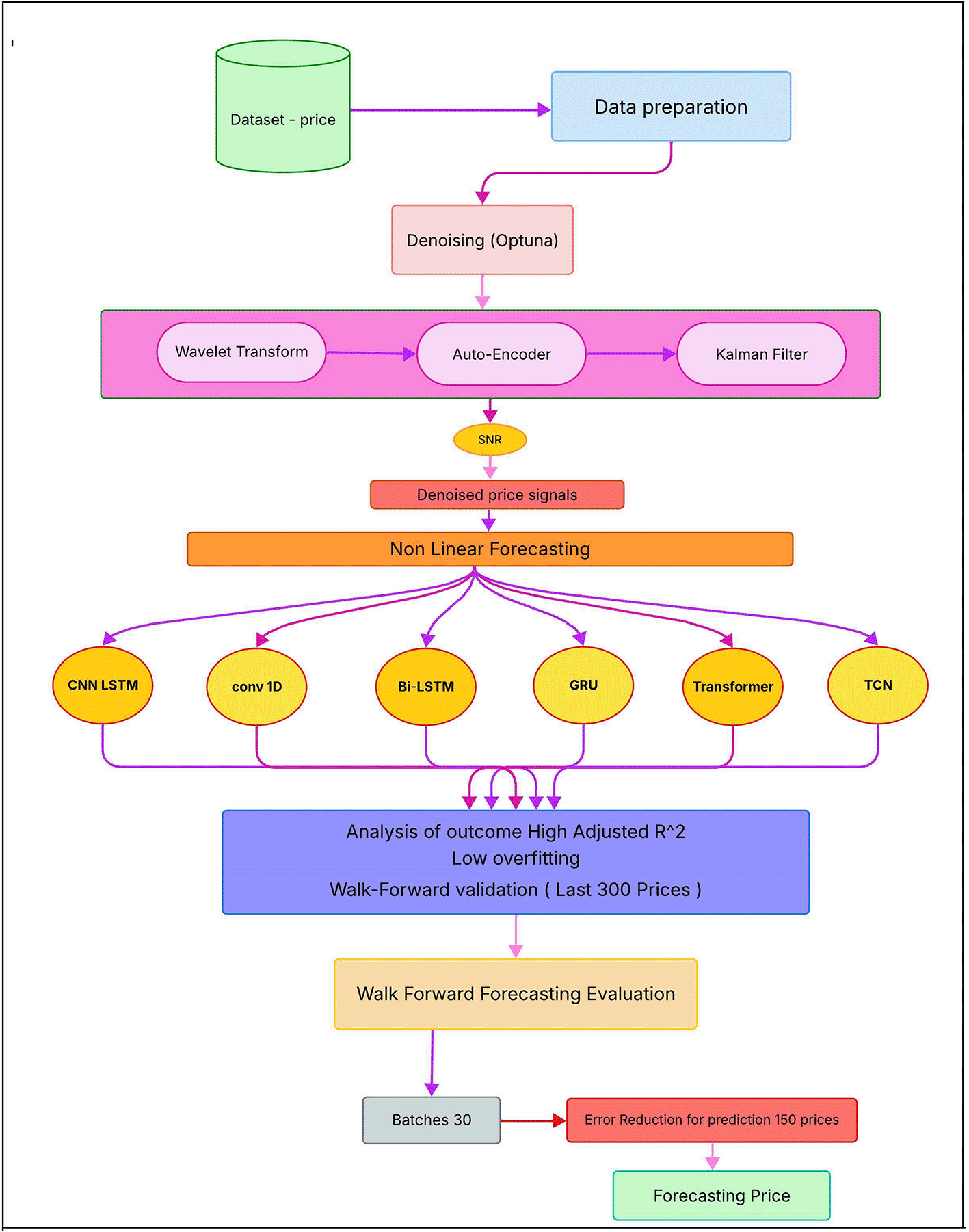
This flowchart illustrates the various steps of the extensive step-by-step methodology used in this study, from initial data gathering and K-means clustering to signal generation and walk-forward validation.
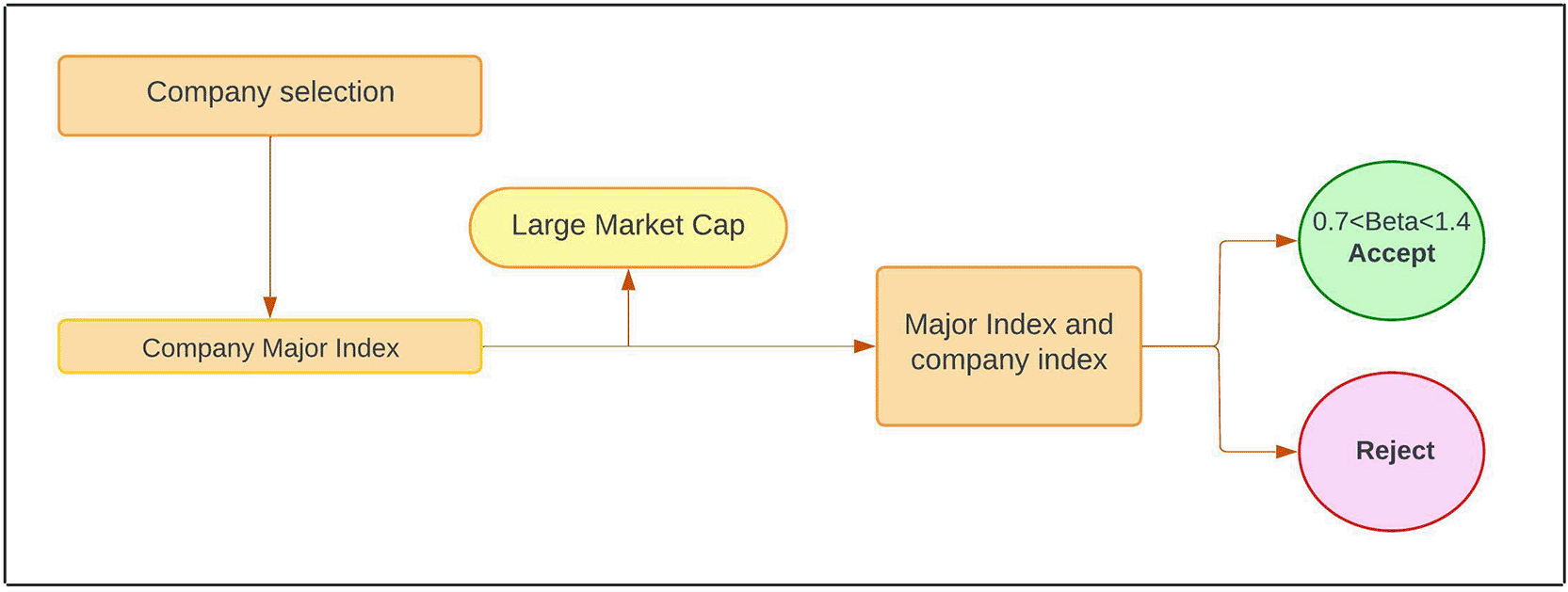
We first assemble the dataset by targeting the six equity markets of interest. Using Yahoo Finance, minute-level OHLC and volume data are downloaded for each market’s primary exchange. Within each country, we select the 20 largest companies by market cap and download their latest price series. To ensure representative sampling of market movements, the 30-day rolling beta of each stock relative to its relevant index (e.g., S&P 500, N225, STI) is computed, and stocks with high or low beta are noted. Only large-cap stocks with full data having consistent trading histories are retained for analysis.40
Table 2 shows the balanced portfolio of high-liquidity stocks, selected across developing and developed markets (USA, Japan, Singapore, India, Brazil, Malaysia), and provides details of the tickers and their respective market cap ranges in each, which form the basis for the modelling presented later. Retrieve OHLC (Adjusted close) data at the minute level for a selection of stocks through Yahoo Finance and ensure that approx. 30 trading days are gathered for each stock in the market.
Table 3 gives a small glimpse of the raw, minute-level OHLC prices, showing the high-frequency temporal structure before the implementation of our denoising pipeline:
The method generates information for each of the six target markets (developed: US, Japan, Singapore; developing: India, Brazil, Malaysia), shortlists ~20 large-cap stocks by market capitalisation. Compute a 30-day rolling beta against the local benchmark index to ensure broad market representation. Only stocks with complete, high-quality data were retained.40 It’s also observed that, for developing countries, selecting companies with strong financial ratios provides a sound basis for effective financial support and portfolio-based prediction.43 An example of a sequential multi-stage denoising pipeline using Discrete Wavelet Transforms, a Variational Autoencoder, and Kalman Filters to produce a clean prediction is shown in Figure 2.
A conceptual flowchart of the sequential multi-stage denoising pipeline combining Discrete Wavelet Transforms, Variational Autoencoders, and Kalman Filters.
Prior to modelling, each raw price series is converted to log-returns and normalised. Minute-level data are notoriously noisy, so we implement a three-stage denoising strategy.
I. Denoising: The study converts raw minute-bar price series to log-returns and normalises. Apply a sequential multi-stage denoising pipeline combining
The hyperparameters for each denoising stage (wavelet type, decomposition level, threshold λ; VAE architecture; Kalman noise covariance) are automatically optimised using the TPE sampler in the Optuna library to maximise the signal-to-noise ratio.36
Figure 3 shows how, during the optimisation phase, the specific data transformations are applied, and how Optuna and Wavelet transforms help to filter out microscope noise.
To effectively capture the underlying market dynamics without the distortion caused by microstructure noise, this study extracts the true trend using the Smoothed Sequence approach, following the methodology established by.32 By continuously adjusting to the market, this method filters out transient volatility and isolates the actual price trajectory. Specifically, for a given time series of raw stock prices , the smoothed sequence utilising a window size of is computed as follows32:
Where, represents the smoothed value; it moves in the same direction as the market to reflect the true trend. By extracting this smoothed sequence, we ensure that the deep learning models that follow are fed data that reflects true market movements, not erratic movements driven by high-frequency noise.
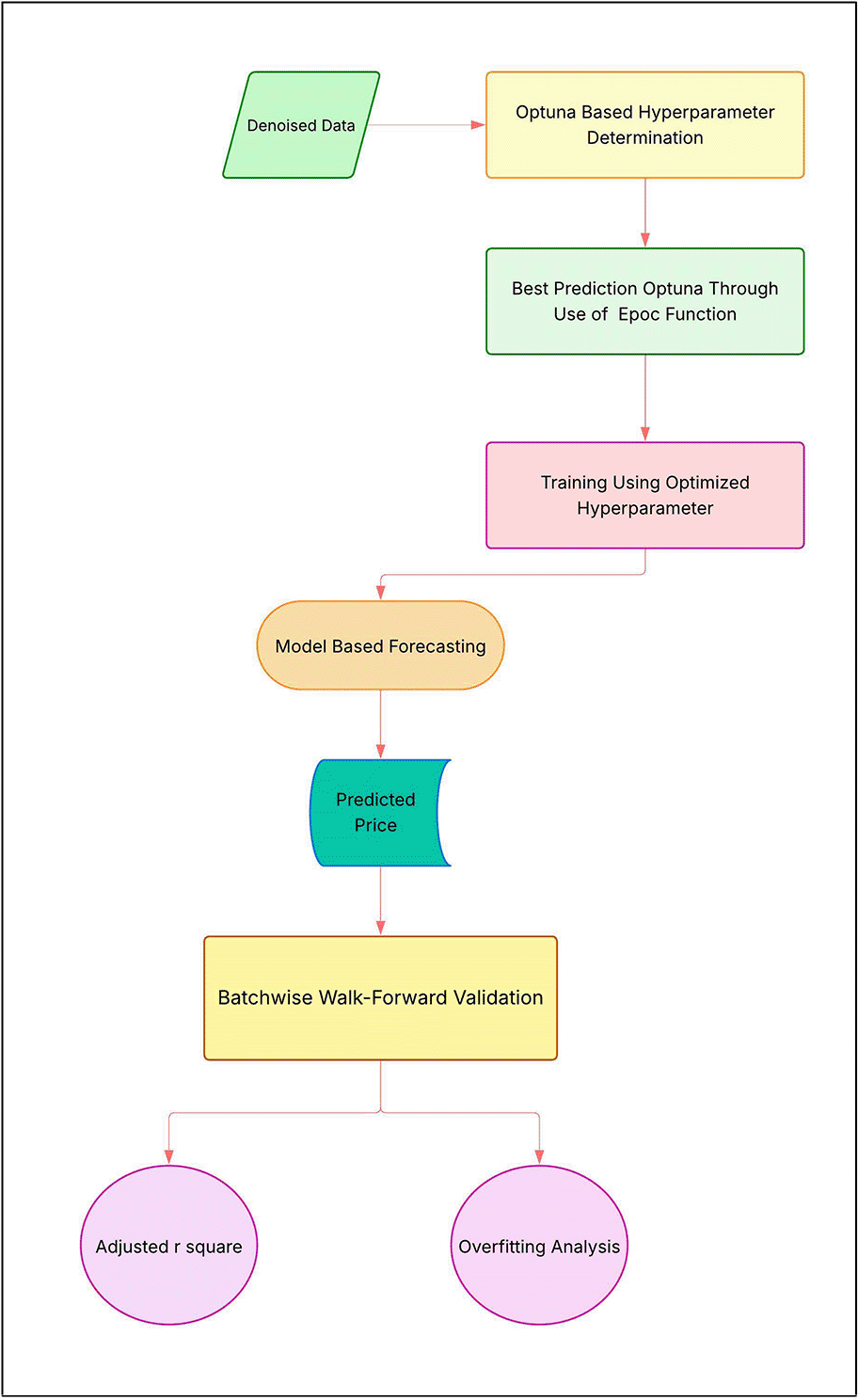
II. Model Training: The research then tests six advanced deep learning models on the denoised univariate price series - 1D Conv-LSTM, CNN-LSTM, Gated Recurrent Unit (GRU), Bidirectional LSTM (Bi-LSTM), Temporal Convolutional Network (TCN) and Transformer (self-attention). Each model has a very simple architecture: 30 past log-returns with a 30-minute time window to forecast the next-minute intensity, with 2 stacked hidden layers, 20% dropout, Adam optimiser, and Mean Squared Error loss. No traditional technical indicators are used; only the pure price signal is focused on.2,22
Figure 4 outlines the structural framework of the six deep learning models utilised in this study, detailing the 30-minute input windows, hidden layers, and evaluation checkpoints.
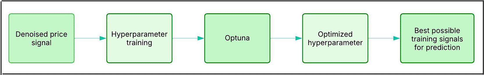
Figure 5 visually illustrates the discrete wavelet transform (DWT) process, showing how the raw signal is split into coarse and detail coefficients.
III. Walk-Forward Validation: We then employ an expanding-window (rolling origin) walk-forward validation: at each step (~300-minute trading day), retrain all models on all past denoised data and test on the next out-of-sample block. The process records performance metrics at each step: adjusted R2 (typically 78–95%) and overfitting ratio (<10%) on the validation block. Finally, generate the held-out 150-point forecast and evaluate its risk-adjusted return.
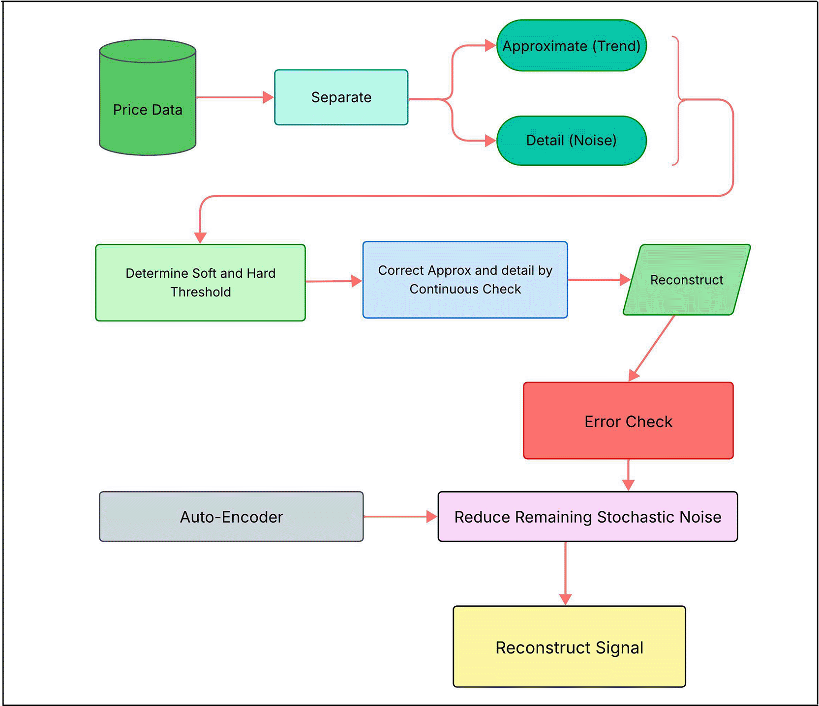
First, a Discrete Wavelet Transform (DWT) using Daubechies wavelets decomposes the return series into coarse (approximation) and detail coefficients. Specifically, at the level , the transform is given by convolutions with a low-pass and high-pass filters32,44:
The process essentially classifies the true noise sequence referenced by high-pass g [n] as high-frequency price signals from real low-pass h [n] signals. The methodology trains on real price movements that are repetitive and train-worthy and is intended to be retained in the neural network for real sequence-based price movement applications. Soft-thresholding is then applied to the detail coefficients to suppress high-frequency noise45:
1) Variational Autoencoder (VAE)
Next, the partially denoised series is passed through a Variational Autoencoder for nonlinear noise removal. The VAE consists of an encoder mapping the input return to a latent distribution , and a decoder reconstructing from the latent sample . Training maximises the evidence lower bound (ELBO) on the log-likelihood46,47:
2) Kalman Filter
Finally, we apply a Kalman filter to the VAE output to smooth any remaining microstructure noise. We model the log-return series as a linear Gaussian state-space system: the state (true return) evolves as and the observation is , where are Gaussian noises. At each time step, the filter performs a.48,49
Here, is the error covariance, Q, R are the process/measurement covariances, and is the Kalman gain. This recursive filtering yields a final smooth state estimate that forms the clean price signal used for forecasting. Overall, the combination of DWT, VAE and Kalman filtering is an effective approach in amplifying the true signal by absorbing noise sequentially, both high-frequency and model-based noise.
In the forecasting stage, we deploy six state-of-the-art deep learning architectures, each designed to capture temporal patterns in the denoised price series. Specifically, we implement:
1) Convolutional Neural Network (CNN-1D)
CNN-1D s extract short-term local features via convolutional filters. For an input sequence and a filter of size , the convolution output (feature map) at time is50,51:
Where, is a nonlinear activation (e.g., ReLU) and is a bias term. Stacking such filters allows the model to detect salient intraday patterns (e.g., recent spikes or dips).
2) Gated Recurrent Unit (GRU)
The GRU is a recurrent network that controls information flow via update and reset gates. The equations are52:
Where, is the input at time , the previous hidden state, and the sigmoid function. The update gate blends the old and candidate states, while the reset gate controls how much past information to forget.
3) Long Short-Term Memory (LSTM)
The LSTM is similar but uses separate input, forget, and output gates to mitigate vanishing gradients. Its core equations are53:
Here, is the cell state storing long-term memory, updated by the forget ( ) and input ( ) gates, and is the hidden output gated by .
4) Temporal Convolutional Network (TCN)
The TCN uses causal dilated convolutions to capture very long-range dependencies. For a dilation factor and filter size , the dilated convolution at position is27:
By stacking layers with exponentially increasing , the receptive field grows exponentially, allowing the TCN to learn long-term patterns without recurrences.
5) Transformer (Self-Attention)
The Transformer model relies on self-attention to weight all past observations when forecasting. The core scaled dot-product attention is54:
All denoising hyperparameters (wavelet family, autoencoder bottleneck size, and Kalman covariances) and model hyperparameters (learning rates, layer sizes, and dropout rates) are tuned using Optuna to ensure optimal performance on a held-out validation split. In total, these six architectures encompass both convolutional, recurrent, and attention-based approaches, each expected to capture different aspects of intraday dynamics. We exclude other methods (e.g., technical indicators or simpler ML models) to focus on these well-established deep learning models, which are known to capture nonlinear patterns in financial time series.
Each forecasting model is trained end-to-end on the Optuna-denoised price series. We use a consistent configuration: two hidden layers (e.g., two LSTM layers or two convolutional stacks), 20% dropout to mitigate overfitting, and the Adam optimiser with mean-squared-error loss (as in25). The input to each model is a fixed-length window of 30 past log-returns, and the output is the predicted next-minute return. Training proceeds on the expanding set of historical data, as in walk-forward validation; no cross-market data leakage is allowed. This uniform architecture facilitates a fair comparison of model performance across markets and ensures that any differences arise from market characteristics rather than model design.
To rigorously assess forecasting accuracy in a simulated real-time setting, we use expanding-window (walk-forward) evaluation. At each validation step (approximately 1 trading day, ≈300 minutes), all models are retrained on the cumulative denoised data up to that point and then tested on the immediately following out-of-sample block. This process is repeated until the end of the sample, yielding an out-of-sample forecast for each step. We record the adjusted of each one-day forecast (typically 78–95%) and monitor overfitting by comparing training vs validation error (overfitting ratio < 10% indicates well-generalised models).
Finally, the last 150-minute forecast (simulating the final day) is used to compute trading performance. In each market, we generate long/short signals based on the predicted returns and form a capital-weighted portfolio. We then compute the risk-adjusted return using the Sharpe ratio, defined as
Market-specific risk-free rates are based on the prevailing 10-year government bond yields (e.g., ~6.65% in India, 13.88% in Brazil, and 3.58% in Malaysia at the end of 2025). All yield estimates are drawn from5,55 for consistency. A Sharpe ratio above 1 is considered a favourable risk-return tradeoff. The above procedures ensure that our evaluation reflects true out-of-sample performance, free from look-ahead bias.
Forecasting on minute-level stock prices is inherently challenging because the raw price series are dominated by short-term noise - for example, in the case of short-term noise due to bid-ask spreads and imbalances in the order book - more so than by stable predictive structures.56 Our raw data from Yahoo Finance exhibit erratic behaviour and a high degree of non-stationarity in mean and variance, which limits the ability of standard linear time-series models to a great extent.57–59 As a result, we utilise nonlinear deep learning architectures and a growing walk-forward retraining strategy to extract weak yet economically relevant signals and maintain forecast validity during rapid regime changes.2,25,60
To explore the complex parameter spaces in our pipeline, we use Optuna, an automated hyperparameter optimisation tool based on Tree-structured Parzen Estimators (TPE).36 Optuna has been used in two separate stages: first, to optimise the signal-to-noise ratio for denoising (optimise the parameters of wavelets, autoencoders and Kalman Filters) and second optimize the prediction error on a dataset not included in the training (optimise the learning rate, the number of layers and the dropout procedure in the Deep Learning models). This automated, define-by-run approach is crucial for managing mutually dependent factors and ensuring resource efficiency when manual grid search would be impractical computationally.
Three complementary denoising techniques are used in order to suppress microstructure noise while retaining economic signals. First, Wavelet transformations (e.g. Daubechies) to deconstruct the series to suppress high frequency coefficients by soft-thresholding (for the purpose of effectively filtering the irregular noise but retaining underlying dynamics.32,61 Second, denoising autoencoders generate a compressed latent representation because the reconstruction process imposes compression, separating main price signals from random variations.62,63 Third, Kalman filters are recursive state-space estimators that smooth the series by adapting to changes in volatility without using fixed window lengths.64,65 Collectively, these methods, tuned with Optuna, improve the signal-to-noise ratio by amplifying meaningful short-term movements that are important for the model’s predictive accuracy.
We use deep sequence models (including such models as TCN, GRU, LSTM (both standard and bidirectional), and hybrid architectures of CNN-LSTM/Transformer). Through such modeling we can forecast denoised minute-level movements. By contrast with the traditional linear methods of financial time series analysis (e.g., ARIMA), these nonlinear models account for nonstationary dynamics and complex dependencies, which have long been neglected by old-fashioned statistical tools or shallow neural networks.25,66
RNN-based models (LSTM, GRU) use gates to learn long-term temporal dependencies while filtering out noise. Hybrid CNN–LSTM architectures are more effective than these: with convolutional layers, they can transform inputs into deeply learned local views before processing them as sequence data.34 Temporal Convolutional Networks (TCN) leverage both dilated causal convolutions for efficient long-range memory (Bai et al., 2018) and Transformers, which utilise self-attention to capture volatility clustering and regime transitions.66 Studies have now confirmed that fitting these methods to transient patterns characteristic of intraday markets has significantly improved risk-adjusted returns and reduced RMSE.67
The deep learning models, i.e., LSTM, Bi-LSTM, GRU, TCN, Transformers, Conv1D-LSTM, and CNN-LSTM, were developed using denoised minute-level stock price data in a walk-forward validation. Hyperparameters were optimised using the Optuna optimisation library, and for microstructure noise denoising, wavelet transform, autoencoders, and Kalman filters were used sequentially.
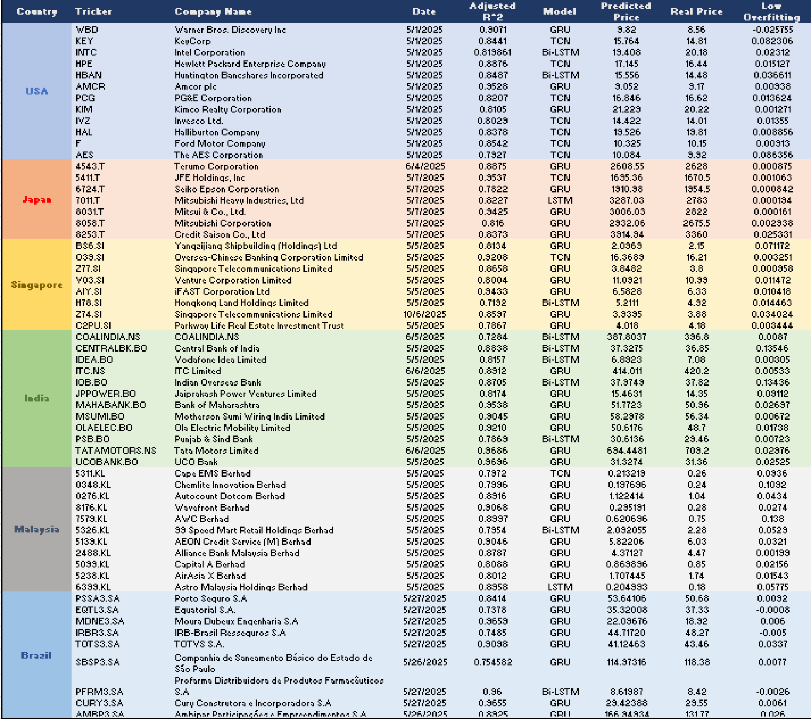
Figure 6 shows the detailed breakdown of deep learning forecasting results in both developed and developing markets. It shows the top performing stocks based on the country, the ticker, the company name, the date and the adjusted R2, the best model, predicted price for the stock, the real price, the high predictive accuracy (Adjusted R2) and low overfitting rates of the various models in terms of predicting and comparing forecasted prices with actual intraday market data. Although a high adjusted R2 indicates good predictive performance, financial processes with high variance can be justified by good predictive hyperparameters.68
Stock selection for inclusion in the portfolio was based on the highest adjusted R2 values (indicating the strength of the model’s predictions against real prices) and the lowest overfitting value (the difference between the training and validation R2, kept below 10%).
To further ensure that the quality of stocks and the strength of exploitable patterns in denoised data were sufficient, we calculated the Signal-to-Noise Ratio (SNR) for selected stocks. In the context of finance, SNR measures the ratio between structured, predictable price movements (signal) against the random microstructure movement (noise), and is borrowed from signal processing. Higher SNR implies cleaner, more reliable forecasting signals - especially important in developing markets where there is typically greater inherent volatility, but also exploitable inefficiencies.
Table 4 compares the initial Signal-to-Noise Ratios (SNR) across the selected assets in developing markets’ imperialistic environments, illustrating the micro-structure noise present in volatile environments.
Table 5 summarises the Signal-to-Noise Ratios (SNR) of large-cap stocks from developed markets as a baseline for clarity, compared with those from developing economies.
We used inverse-volatility weighting to construct portfolios from the best models’ buy/sell signals. In simulated trading, there was a set amount of money to start with (for example, $1,000) over 30 days. The forecasts were for 150 minutes of the day, and the rules were realistic.
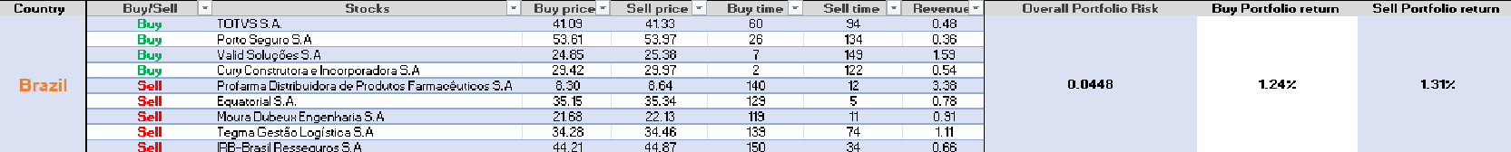
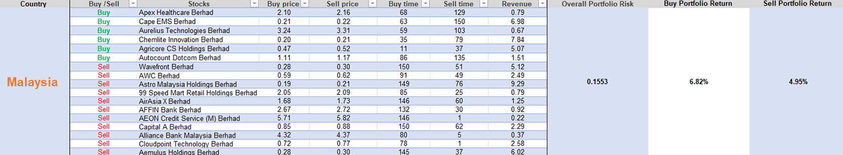
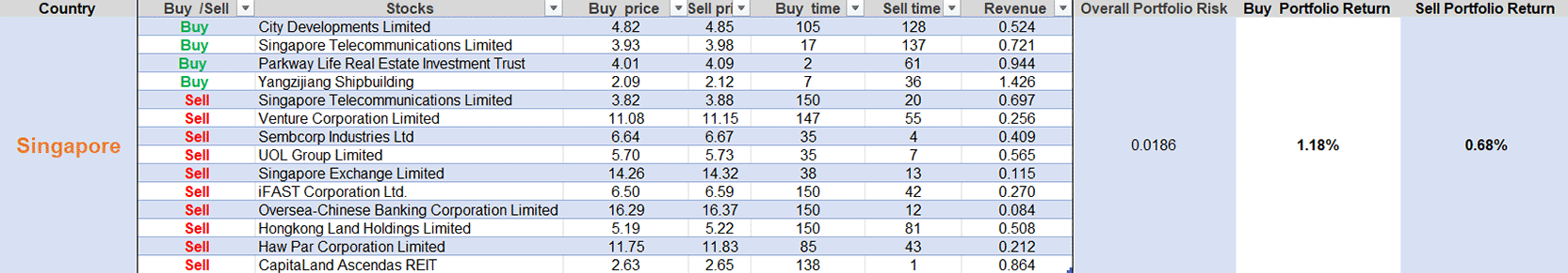
Table 6 details the outcomes of the 30-day simulated intraday trading strategy. The results demonstrate that developing markets yielded substantially higher Sharpe ratios and raw profits compared to their developed counterparts.
In this part, we present the results of the portfolio optimisation procedure applied to the predicted minute-level stock prices in both developed (USA, Japan, Singapore) and emerging (India, Brazil, Malaysia) markets. We used a conventional pipeline based on denoised high-frequency data and deep learning predictions, using models including LSTM, Bi-LSTM, GRU, TCN, Transformers, Conv1D-LSTM, and CNN-LSTM to optimise. The final portfolios included stocks with the best adjusted R-squared values (78%–95%, with an average of about 85%) and the least overfitting (less than 10%). This was confirmed using walk-forward testing.
The hyperparameter optimization within our deep learning architectures was specifically designed to test and lock onto the true market trajectory provided by the preprocessed data. Because the models were trained on the Smoothed Sequence,32 they captured the underlying trends rather than overfitting to random market fluctuations. This ability to map real price movements directly accounts for the robust predictive performance, yielding Adjusted R2 scores ranging from 75% to 95% across the tested assets. Without this smoothed sequence isolating the true trend, predicting the real price movements with such high accuracy would not have been possible.
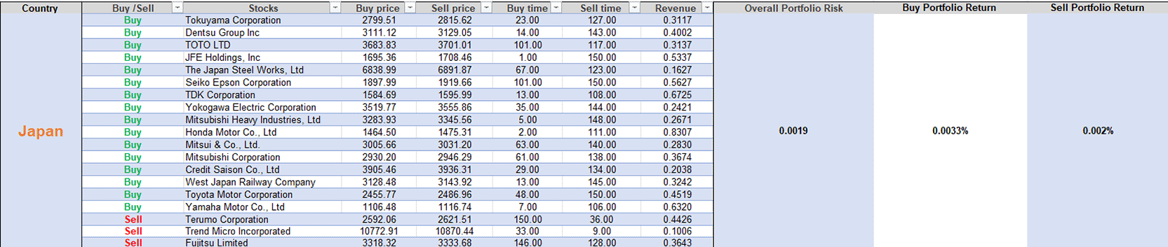
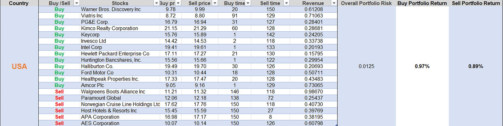
The portfolios were built separately for buy (long) and sell (short) positions. To lower risk and raise returns, they were weighted by inverse volatility. We did conduct some behaviour, such as simulating intraday trading with a projection horizon of 150 minutes, starting from an initial amount included in the model and considering realistic limitations, such as transaction costs (implicit in returns) and liquidity. The standard deviation of returns is used to estimate the portfolio’s total risk. Buy-and-sell portfolio returns are shown as percentages. Developing markets consistently showed higher Sharpe ratios (1.2–1.6 times those of developed markets), with buy-side Sharpe ratios of 1.9–5.3 versus 1.0–1.4 in developed markets, highlighting superior risk-adjusted performance driven by exploitable inefficiencies. We include the best portfolios for each country below. These include buy selections, company names, buy/sell prices, timing (in minutes), revenues, overall portfolio risk, and buy/sell portfolio return.
Figures 7 through 12 are visual maps that plot the optimised buy-and-sell portfolio for each market. These charts show the exact timestamps of each trade, how assets were allocated to them, and the expected intraday returns over the simulated 150-minute horizon.

The results confirm that deep learning on denoised minute-level data translates inefficiencies in developing markets into superior risk-adjusted intraday returns, thereby challenging investor bias toward the stability of developed markets.69 Equivalent forecasting accuracy, but significantly greater tradability in India, Brazil and Malaysia, demonstrating the Adaptive Market Hypothesis, which posits higher practicability of computational improvements in exploiting anomalies in less efficient environments.1,2
This is an advantage over weaker returns that come with higher equity risk premiums in emerging markets,5 for risk that is well compensated for (volatility, etc) but that provides alpha where noise is managed. The absence of technical indicators isolates pure price dynamics and makes the study more generalizable, which is rare for intraday.25
The empirical results of this study validate the efficacy of data denoising combined with advanced deep learning architectures for high-frequency price forecasting. For all six of the markets analyzed, the predictive models provided a good level of accuracy with adjusted R2 scores ranging from 78–95% (average ~85%). Crucially, the walk-forward validation implementation ensured that overfitting remained well below 10%, ensuring that the models reflected generalizable market patterns rather than ephemeral market noise.
When these predictive signals were converted into inverse volatility-weighted trading portfolios over a 150-minute intraday horizon, there was a clear difference in performance between the market types. The portfolio optimisation analysis showed that developing markets (India, Brazil and Malaysia) achieved a significant risk-adjusted gain relative to developed markets (USA, Japan and Singapore). Developing markets produced buy-side Sharpe ratios that ranged from 1.9 to 5.3, which were 1.2 to 1.6 times higher than the 1.0 to 1.4 Sharpe ratios recorded in mature markets. Ultimately, these results from the portfolio bear out that the microstructure volatility inherent in the developing world can be managed and exploited, providing an alternative, highly lucrative allocation of short-term alpha for investors to counter traditional ‘flight to safety’ biases.
In practice, the framework offers retail and institutional investors a replicable tool to reallocate to liquid emerging large-cap stocks, which could potentially improve diversification and returns given saturation in developed markets. Limitations include the short 30-day test period and reliance on historical data; future work could consider longer horizons or account for transaction costs.
Overall, deep learning breaks down creative-market jargon because in these developing economies, it shows underserved qualities and there is a lot for more exposure to be fluent for better, more efficient portfolio.3,4
Although this study provides empirical evidence of the efficacy of deep learning on denoised minute-level data for intraday forecasting in a developing market, there are certain limitations that must be recognised.
First, the analysis is based on a rather limited 30-day trading period. Although the look-ahead bias is reduced by the walk-forward validation method, this limited horizon does not necessarily eliminate regime shifts, structural changes in markets, or exceptional events (e.g., global crises) that may affect the patterns of inefficiencies.1,69 The data’s robustness would improve by extending it over a multi-year span.
Second, simulated trading portfolios do not account for transaction costs, slippage, or market impact, which are particularly pronounced in high-frequency, minute-level strategies. In less developed financial markets, such as India, Brazil, and Malaysia, lower liquidity and wider bid-ask spreads can severely erode realised returns.41 In the real world, some portions of the portfolio might not actually generate the Sharpe ratios quoted here.
Third, the denoising pipeline (combination of wavelet transforms, variational autoencoders and Kalman filters), although optimized using Optuna, the risk of over-denoising or removing economically meaningful high frequency signals (e.g. microstructures dynamics critical for intraday alpha)32,56 are adjusted with proper trend pick up and drop off which is essentially achieved as well but heavy market shocks cannot preserve the require information; Parameter sensitivity and possible signal distortion are still challenges in sequential denoising methods.
Fourth, stock selection targeted the large-cap stocks in the liquid markets and excluded thinner or more volatile segments. This can be an overestimate of exploitable inefficiencies, as the smaller the stock or what is excluded (e.g., from developing regions), the greater the political risk and the lower the predictability.5 This process essentially ignores Fama French model, suggest against small market gains are against large-cap stocks in the long run.70
Finally, adjusted R2 and Sharpe ratios show strong performance; the results are based on historical data from Yahoo Finance, which may include survivorship bias or adjustments that are not 100% indicative of live trading conditions. Overfitting (even with walk-forward validation and reported small gaps (<10%)) is a potential issue for deep learning models trained on noisy financial series.10,38
These limitations point to directions for future research, including the inclusion of transaction costs, longer horizons, testing in real time for execution, and extending to additional markets or hybrid denoising techniques.
Not applicable. This study utilises publicly available, secondary market data and does not involve human participants or animal subjects.
• Source Code: The full code pipeline for data denoising (Wavelet/Autoencoder/Kalman), model training, and portfolio simulation is available at: https://github.com/Monjur1841/minute-level-stock-forecasting
• Archived source code at time of publication: https://doi.org/10.5281/zenodo.19014187
• License: OSI-approved MIT License.
| Views | Downloads | |
|---|---|---|
| F1000Research | - | - |
|
PubMed Central
Data from PMC are received and updated monthly.
|
- | - |
Provide sufficient details of any financial or non-financial competing interests to enable users to assess whether your comments might lead a reasonable person to question your impartiality. Consider the following examples, but note that this is not an exhaustive list:
Sign up for content alerts and receive a weekly or monthly email with all newly published articles
Already registered? Sign in
The email address should be the one you originally registered with F1000.
You registered with F1000 via Google, so we cannot reset your password.
To sign in, please click here.
If you still need help with your Google account password, please click here.
You registered with F1000 via Facebook, so we cannot reset your password.
To sign in, please click here.
If you still need help with your Facebook account password, please click here.
If your email address is registered with us, we will email you instructions to reset your password.
If you think you should have received this email but it has not arrived, please check your spam filters and/or contact for further assistance.
Comments on this article Comments (0)