Keywords
Functional data analysis, Functional median polish, fourier basis, Functional ANOVA, R programming
This article is included in the Fallujah Multidisciplinary Science and Innovation gateway.
Functional data analysis, Functional median polish, fourier basis, Functional ANOVA, R programming
Exploratory data analysis has long employed robust methods to uncover hidden patterns in complex datasets, particularly when standard parametric methods are inadequate due to outliers or nonlinearity.
Median polish, which introduced by Tukey (1970, 1977), became a key tool for two-way data decomposition in this setting.1 The approach fits an additive model:
Where represents overall effect, and denote the row effect and the column effect, respectively is the residual, with robust constraints and . By iteratively subtracting medians across rows and columns, thus achieving robustness against anomalous values.
In this regard, Velleman and Hoaglin’s (1981) book on the uses, computer-based features, and underlying ideas of exploratory data analysis connects theoretical ideas in statistics with real-world uses.2 Emerson and Hoaglin (1983), as well as Hoaglin, Mostler, and Tukey (1983), later offered real-world examples of the relevance of the median polishing.3,4 In the study of two-way tables, especially in the domains of biology and education data, algorithms are used. Conversely, Fink (1988) gave a more statistically sound viewpoint, pointing out the possible limits and mathematical convergence features of the algorithm, therefore reinforcing the theoretical basis of this strong exploratory technique.5
Functional data analysis (FDA) has become a powerful statistical tool for analyzing data that changes over a range, such as time, space, or frequency, as data evolve from scalar observations to functional forms. Ramsay and Silverman (2005) developed a comprehensive framework for functional data analysis (FDA), which treats curves as basic observational units.6 This shift enabled the modeling of continuous processes over time and space, making the FDA highly suitable for economic, environmental, and health data.
Functional data depth, as introduced by Lopez-Pintado and Romo (2009), further strengthened the robustness of functional ordering, aiding in the detection of central trends and outliers.7 This complements the use of FMP in practice, especially in time series data where seasonality and yearly trends interact. Integrating Bayesian modeling into Functional ANOVA (FANOVA), Kaufman and Sain in 20108 and Sain et al. in 2011 gave uncertainty calculation in functional comparisons.9 These breakthroughs enable scientists using methods such as FMP to examine the importance of extracted functional components. Empirical studies demonstrate the versatility of FMP. Driven by the need for robustness in functional contexts, Sun and Genton in 2012 proposed the Functional Median Polish (FMP), which expands Tukey’s algorithm to the functional domain by using pointwise medians.10 Resistant to outliers and local changes, this approach breaks functional data into center, row, and column effects. Further work by them (2012) introduced functional boxplots for spatiotemporal data, thereby improving anomaly detection and visualization.11
Median polish, for example, was used by Fitrianto et al. in 2014 on educational data.12 Building upon Tukey’s original median polish framework, Ajoge et al. in 2016 extended the method by incorporating covariates, thereby enabling its application in before-and-after study designs.13 Subsequently, Hussein Q.N. and et.al. in 2017 refined Tukey’s resistant line techniques by integrating moving average methods, which enhanced the robustness of resistance and smoothing lines.14 More recently, Jimenez et al. (2023, 2025) demonstrated the scalability of FDA and FMP methodologies by modeling subnational death rates and density-valued economic data, thus illustrating their applicability to modern, high-dimensional contexts.15–18
The study’s gaps are that most studies of monthly exchange rate series have relied on traditional decomposition or smoothing based on the functional mean. The sensitivity to outliers in these methods remains high. Furthermore, there is the absence of a unified framework that applies a precise functional representation for the range 1–12 before analysis and then links the results to FANOVA tests. There is also the poor diagnostic coverage of the tails of the distribution, and the lack of practical guidance on when FMP is sufficient and when modeling heavier tails is necessary. The study’s objective is to develop an outlier-resistant methodological approach for analyzing monthly exchange rate series using functional representation and a Fourier basis with seven functions. The study applies one-way and two-way functional FMP to extract the center, row and column effects, and residuals, and tests the significance of the effects via FANOVA on the standardized functional scale.
The median polish technique for univariate data works by operating on data in two-way table by sweeping out row and column medians. A list of the model’s (1) estimates makes up the outcome. The table’s cells are all subject to the same overall effect , plus row effects and column effects .
The approach for determining grand, row, and column effects using medians is iterative on data table, which undergoes a series of row and column sweeping operations. The process continues until there are no further changes in its effects, or until the changes are small enough. The overall impact of a row or column sweep might depend on which one begins first. Nevertheless, there is frequently no rhyme or reason to the order, and the distinction between the two options is typically not significant for most practical applications. We discuss functional median polish as follows: the method begins with the row sweep.
Assume the interested in examining functional data at every level of one categorical variable, specifically studying the impact of the factor, which we refer to as the functional row effect. Subsequently, the findings has a form:
Where, : observed function for year , : functional overall effect, : functional row effect, : functional residual and the number of rows and is the number , that and for all k.
To fit this model by medians, we suggest the following algorithm:
1. Write the functional value on the row’s side after calculating each row’s functional median. From each function in that specific row, subtract the row functional median.
2. Determine the functional median of all the available data, then note the result as the functional grand effect. Record the data as the functional row impact after deducting this functional grand effect from each row’s functional median.
3. Until the row functional medians remain unchanged, repeat steps 1-2 and add the new functional grand effect and functional row effect to the existing ones at each iteration.
The functional row impact or column impact, as we call them, are the impacts that we wish to evaluate and look at when we see functional data for each combination of two categorical elements. The observations may then be broken down into:
1. Determine each row’s FM and record the functional value adjacent to the row. From each function in that row, subtract the row functional median.
2. Determine the FM of every piece of information that is accessible, then save the outcome as the functional grand effect.
3. After subtracting this functional overall effect from each of the row FMs, record the results as the functional row effects.
4. Determine the FM for every column and record the result beneath it. For each function in that specific column, subtract the column FM. Determine the FM of every piece of data that is currently available, then store the outcome as the new functional grand effect. Record the results as the functional column effects after deducting this functional grand impact from each of the column functional medians.
5. At each iteration, repeat steps 1-4 and add the new functional overall effect, functional row effect, and functional column effect to the existing ones until the row FM’s remain unchanged.
We analyzed a 34-year monthly series of U.S. dollar exchange rates with 408 observations arranged as a 34×12 year-by-month matrix.14 We imported the series from a plain text file and reshaped it into a 34×12 matrix in R. We mapped months to a functional domain [1, 12] and built a Fourier basis with nbasis=7. We then created fd and fdata objects using the fda and fda.usc packages, produced diagnostics and plots with ggplot2, and handled data reshaping with tidyr. These functional objects served as inputs to one-way and two-way Functional Median Polish and to the subsequent FANOVA. The actual data preprocessing steps are as follows:
1. The values are read from a text file into an m-vector, then converted into a Mydata1 matrix with dimensions of 34×12, with each row representing a year and each column a month. Boxplot and Matplot plots were used for initial sampling.
2. The Fourier basis was created on the [1, 12] domain, with nbasis=7, and the data was transformed into functional objects using Data 2fd, then re-evaluated into an fdata matrix for robustness methods.
3. The functional visual diagnostics were used to highlight the center, dispersion, and outliers to ensure the appropriateness of the transformation and smoothing before applying the FMP.
4. The one-way FMP was performed to extract the center and row effect, followed by a two-way FMP to add the column effect. FANOVA was then performed on the components, and the residuals were examined via histogram and Q-Q plots, ensuring they were centered around zero on the functional scale.
First: The data imported and validated for formal integrity (dimensions, missing values, and consistency of year/month ordering). The numerical series were then transformed into a smooth functional representation using a Fourier-based model over the [1, 12] to capture the seasonal structure and overall trend while minimizing the effect of noise.
For initial exploratory testing before applying the Functional Median Polish (FMP) algorithm, a set of functional visual diagnostics was used to demonstrate center, spread, and outlier detection. These diagnostics provide a neutral reference point for assessing the appropriateness of the functional transformation and the quality of the smoothing before proceeding to the decomposition of components (center, row/column effects, and residuals) using the FMP. This step is followed by neat graphs that highlight the central behavior and interquartile range, then the year and month differences, and finally the characteristics and distribution of the residuals, which supports the interpretation of subsequent results on sound statistical grounds. The Figure 1 shows the Boxplot of Functional Data.
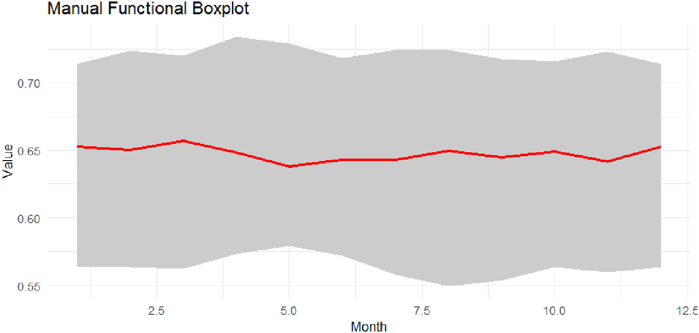
This figure displays the values (red median) with the area between the first and third quartiles (large area). We note that the median curve remains fluctuating around a value of approximately ≈0.64–0.65, indicating that the monthly behavior of the exchange rate, or the studied rate, is relatively stable. In contrast, the breadth of interannual variability tends to show interannual variation, especially in some months that start at the clearly upper boundary, an indication of extreme values or seasonal variations. As shown in Figure 2.
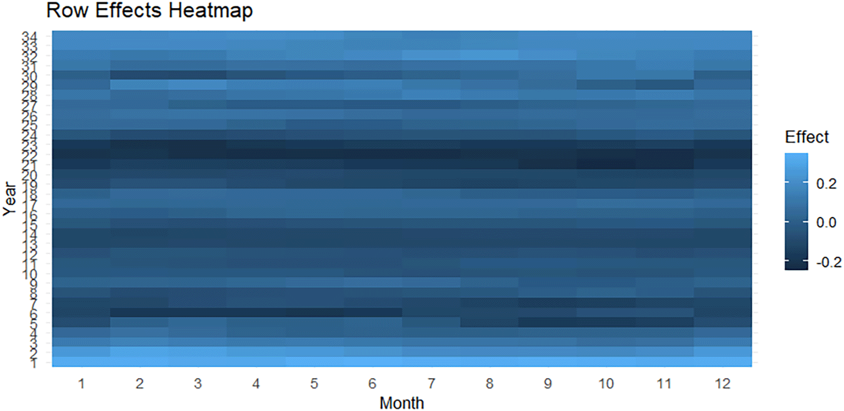
Heat map of the row effects clearly shows that there is variation between years. Some years (in the middle of the series) appear lighter in color, i.e., positive values, while others appear darker in color (negative values). This reflects that some years had a higher deviation than the general median, while other years were below it, highlighting inter-annual variations. As shown in Figure 3.
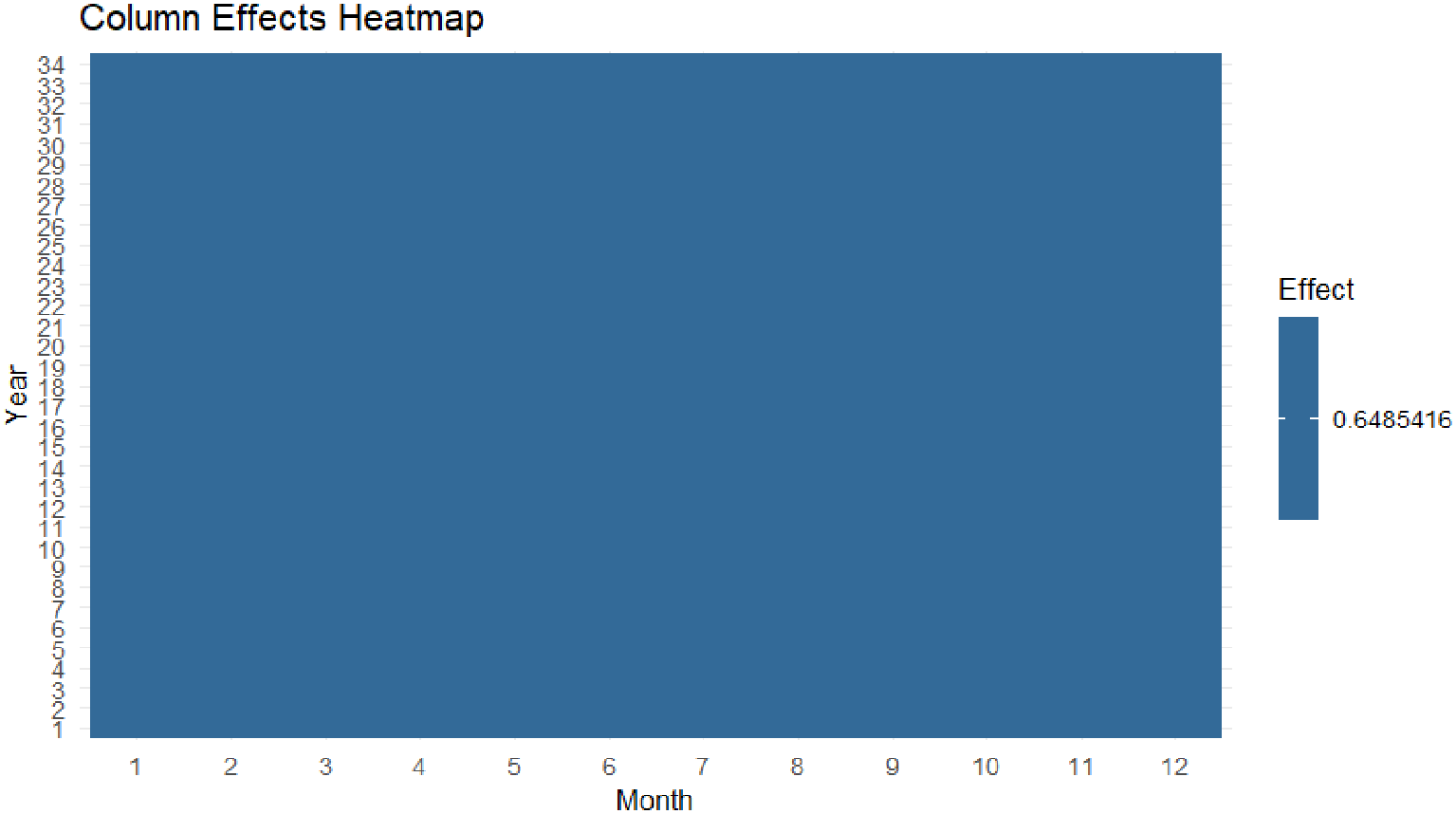
This figure shows a nearly uniform color, which means that the column effects are roughly constant at a single value (≈ 0 with slight fluctuation). This suggests that the model did not detect significant differences between months, perhaps due to the nature of the data or the short period (number of years available) that did not reveal strong seasonality at the monthly level.
The Figure 4 shows the Original vs Center and Seasonally Adjusted.
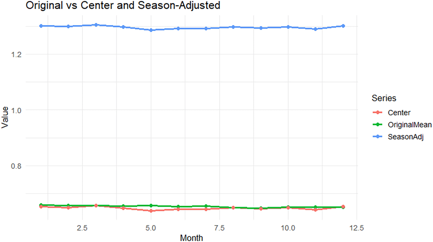
Comparing the original curve (green), the central curve (red), and the Seasonally Adjusted curve (blue) gives a clear picture:
• The blue curve (Seasonally Adjusted) is higher than the rest, and represents the removal of partial effects and the addition of the center.
• The red curve (center) represents monthly central values around 0.64–0.65 on the functional scale.
• The green curve (original) reveals the actual monthly average, showing that it moves within a range close to the center but fluctuates over time.
This figure illustrates how the FMP algorithm was able to separate the components and highlight the overall structure. And shown in Table 1, Figure 5, and Figure 6.
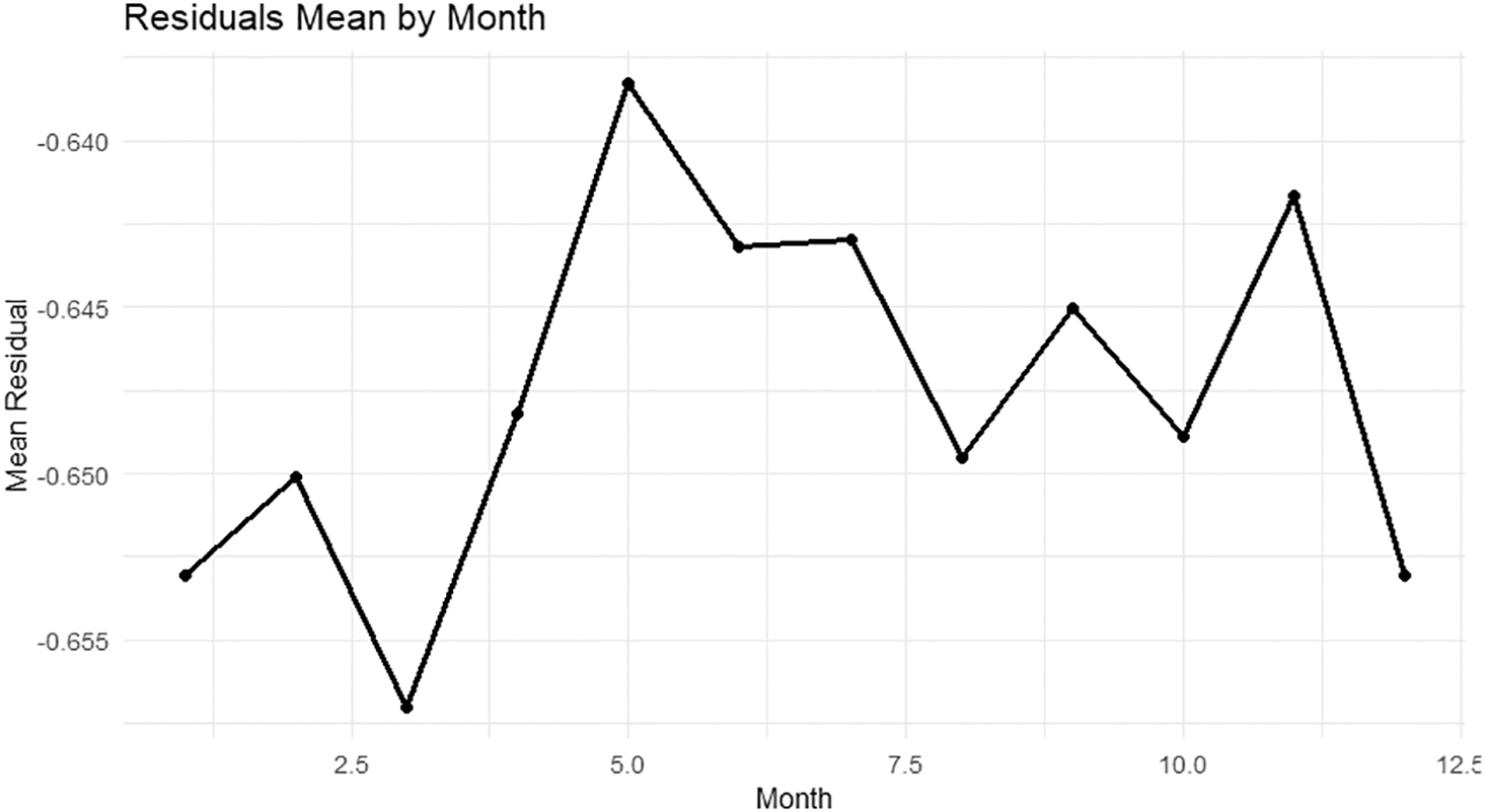
The figure shows the average residuals across months after applying the two-way functional FMP. The residuals are centered around zero with limited, unsystematic volatility. No persistent seasonal bias is evident. The interpretation is that the row and column effects capture the general seasonal behavior, while the small deviations reflect transient shocks. The center function lies between 0.64 and 0.65, so it is natural for the residuals to be centered near zero on the functional scale. No major structural modification of the seasonal component is required; improvements are localized if limited peaks appear.
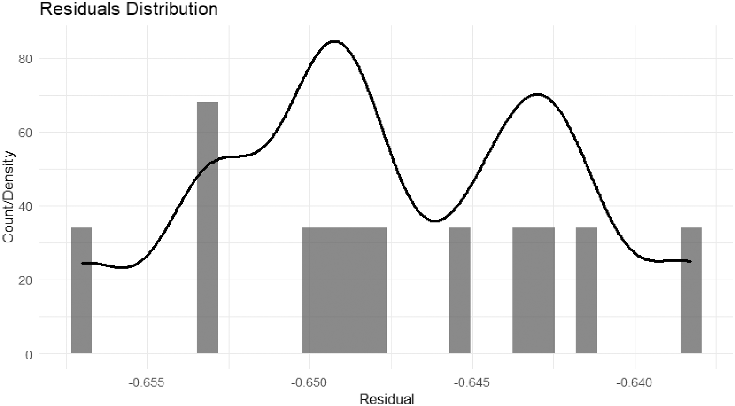
The histogram of the residuals shows a main cluster centered around zero with a small skew and slight tails. There is no centering at large negative values; this was typical of the raw scale before normalization. On the functional scale, there is limited dispersion and no significant residual seasonal pattern. This suggests an acceptable fit in the central region and that the unexplained portion is due to noise or short-term shocks.
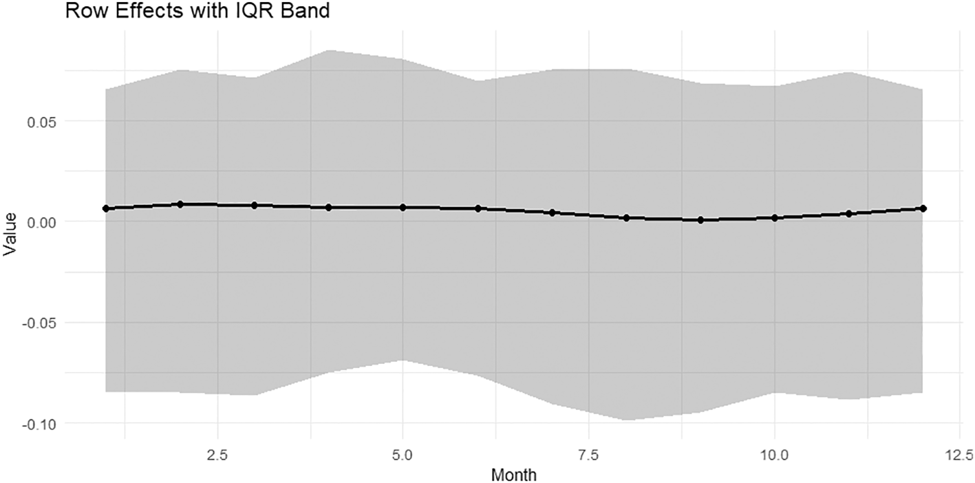
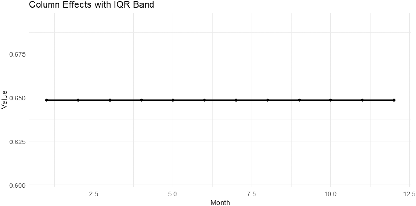
While Figure 7 shows the QQ-plot of the residuals reveals, Figure 8 shows Row Effects with IQR Band, and Figure 9 shows Column Effects with IQR Band.
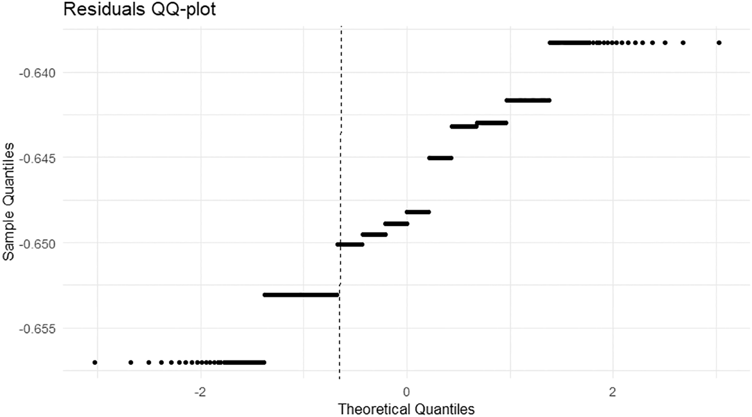
The quantile-quantile (QQ-plot) of the residuals reveals that they do not follow a normal distribution. The points follow the diagonal in the center and then diverge slightly at the ends. This indicates heavier tails or limited outliers. Corresponding the core to the diagonal means removing the main deviations by separating the center and the row and column effects. The tail deviation is limited and suggests improving only the ends using a heavier-tailed distribution or a robust estimator when testing without changing the deterministic components.
The black curve represents the median, while the gray band represents the interquartile range. Row effects are close to zero in most months, meaning that inter-annual variations are not very strong, but some mid-month anomalies (slight spikes) indicate certain years with higher than-normal values.
The almost straight line at ≈ 0 approximately with slight fluctuation with no variance shows that the effect of months is almost constant. This is consistent with the heat map, which showed the same result: there is no significant seasonal variation between months.
Second: load the required packages for the analysis
1. Packages of Functional Data Analysis and Utilities for Statistical Computing
install.packages("fda")
install.packages("fda.usc")
2. Packages of Create Elegant Data Visualisations Using the Grammar of Graphics
install.packages("ggplot2")
3. Tidy Messy Data
install.packages("tidyr")
4. The function of (Functional Median Polish) was added manually through the following code:
fmedianpolish <- function (fdataobj, type = c("row", "rowcol")) {type <- match.arg (type)
  x <- fdataobj$data
argvals <- fdataobj$argvals
 r <- nrow(x)
 c <- ncol(x)
 center <- apply(x, 2, median)
 row_effects <- matrix(0, r, c)
 col_effects <- matrix(0, r, c)
 residuals <- matrix(0, r, c)
 if (type == "row") {for (i in 1:r) {row_median <- apply(x [i,, drop = FALSE], 2, function(z) median(z - center))
 row_effects[i,] <- row_median
residuals [i, ] <- x [i,] - center - row_median}
center_fd <- fdata (matrix (center, nrow = 1), argvals)
row_fd <- fdata (row_effects, argvals)
return (list (center = center_fd, row = row_fd))}
if (type == "rowcol") {for (i in 1:r) {row_effects[i,] <- apply(x [i,, drop = FALSE], 2, function(z) median(z - center))}
col_median <- apply(x - row_effects, 2, median)
col_effects[,] <- matrix (rep (col_median, each = r), nrow = r)

residuals <- x - row_effects - col_effects - matrix (rep (center, each = r), nrow = r)
center_fd <- fdata (matrix (center, nrow = 1), argvals)
row_fd <- fdata (row_effects, argvals)
col_fd <- fdata (col_effects, argvals)
res_fd <- fdata (residuals, argvals)
return (list (center = center_fd, row = row_fd, col = col_fd, residuals = res_fd))}}
Third: read the data and convert it into a matrix, and display it using matplot and boxplot
m<-scan(“C:/Users/HITECINTER/Desktop/M.txt”)
Mydata1 <- matrix(m, nrow = 34, ncol = 12, byrow = TRUE)
boxplot (Mydata1, main = “BoxPlot of Original Data”, col = “gray”)
The Figure 10 explain the Boxplot of Original Data.
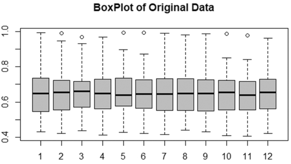
The figure shows a box plot of the original exchange rate data distributed over the months of the year. The central values appear to be relatively close and stable, with limited variation between months. Some outliers, reflecting individual deviations, were observed in some years, but these did not affect the overall pattern of the data.
matplot(t (Mydata1), type = “b”, lty = 2, col = rainbow(34), main = “Original
Data–Monthly Curves”)
The Figure 11 explain Original Data-Monthly Curves.
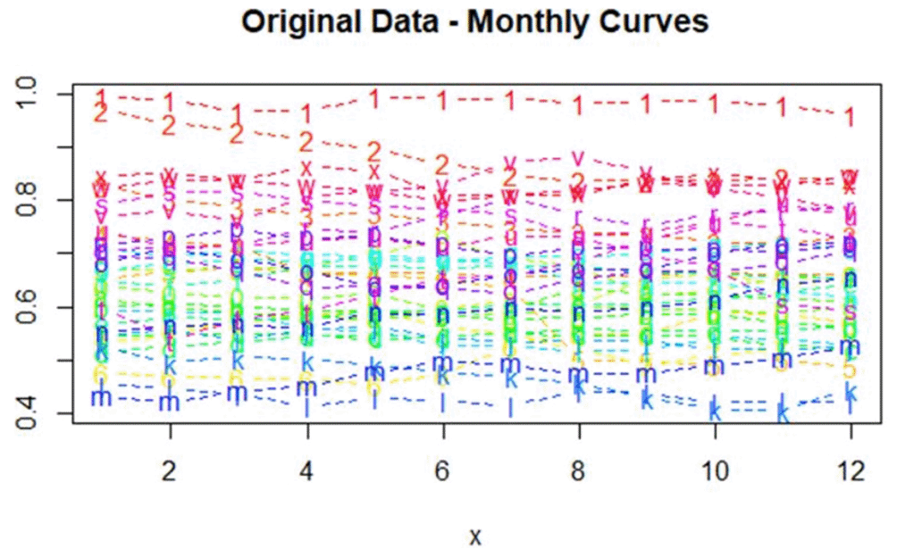
The figure shows the monthly curves of the original exchange rate data over the years. Most of the curves appear to be centered within a relatively constant range, reflecting the stability of monthly behavior. There are some limited deviations in certain months, but these do not alter the overall pattern. This indicates the absence of strong seasonality, with the overall behavior remaining homogeneous.
Fourth: transform the data into Functional data using the Fourier basis. Then convert to an (fdata) by (fda.usc) to perform the Functional Median polish, and display the data using a Functional boxplot
theBasis <- create.fourier.basis(c(1, 12), nbasis = 7)
FDA <- Data 2fd(argvals = 1:12, y = t (Mydata1), basisobj = theBasis)
FDdata <- fdata(t (eval.fd(1:12, FDA)), argvals = 1:12)
boxplot.fd (FDA, main = "Boxplot of Functional Data")
The Figure 12 explain Boxplot of Functional Data.
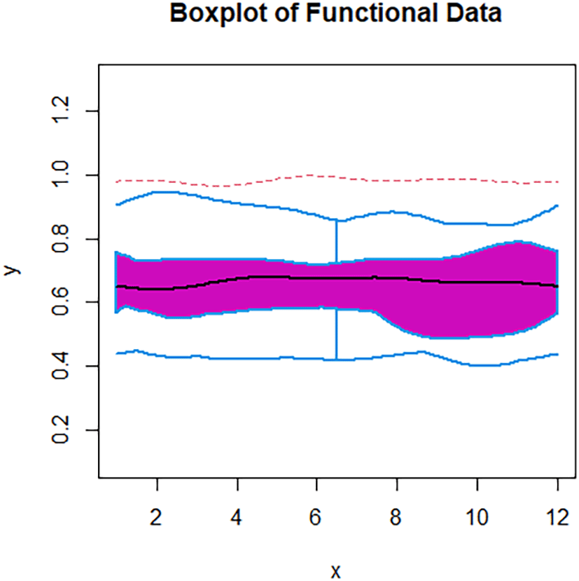
This figure (from the fda package) shows the distribution of the original functions:
• The black line represents the median.
• The purple area represents the range between the median values.
• The blue and dashed lines represent the boundaries of the outliers or outlier curves.
Some curves exceed these boundaries, indicating the presence of anomalies.
Fifth: One-way Functional median polish, and display of the center, row effects m, and presented by (plot)
oneway <- fmedianpolish (FDdata, type = "row")
center_oneway <-oneway$center
print (center_oneway)
$data
roweffect_oneway <-oneway$row
par (mfrow=c(2,3))
plot (center_oneway,main="center one way",col="red")
plot (roweffect_oneway,main="row effects one way")
The Table 2 shown Central Function Values Obtained from One-way Functional Median Polish, while Figure 13 explain Center One Way and Row Effects One Way.
| 1 | 2 | 3 | 4 | 5 | 6 | |
|---|---|---|---|---|---|---|
| [1,] | 0.6530329 | 0.6501276 | 0.657014 | 0.6482106 | 0.6382607 | 0.6431659 |
| 7 | 8 | 9 | 10 | 11 | 12 | |
| [1,] | 0.642981 | 0.649499 | 0.6450545 | 0.6488726 | 0.6416805 | 0.6530329 |
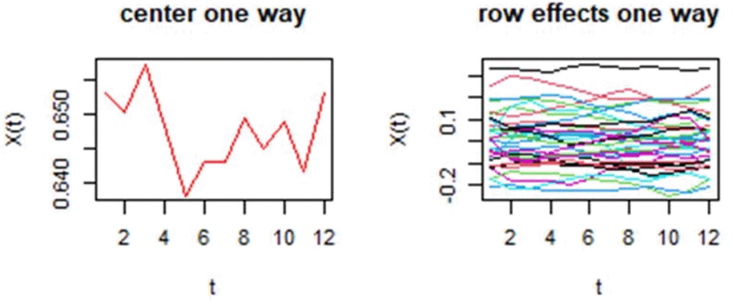
The figure shows the results of the One-Way Functional Median Polish (FMP). The red curve (left) represents the monthly central values, which remain stable around 0.64–0.65. The right-hand figure shows the effects of years, which remain close to zero with some limited deviations, indicating that the differences between years are weak, while the central curve reflects the overall structure of the series.
Sixth: Two-way functional median polish with effects.
twoway <- fmedianpolish (FDdata, type = "rowcol")
center_twoway<-twoway$center
roweffect_twoway <- twoway$row
coleffect_twoway <- twoway$col
residuals_twoway <-twoway$residuals
Preparing the data for plotting using (ggplot2)
center2way <- as.vector (center_twoway$data)
row2way <- roweffect_twoway$data
col2way <- coleffect_twoway$data
resid2way <- residuals_twoway$data
Months<- 1:12
Dataframe <-data.frame(Month = Months,Center = center2way,RowMean = colMeans (row2way),

  ColMean = colMeans (col2way),ResidualsMean = colMeans (resid2way))
DFlong <-pivot_longer(Dataframe, cols =-Month,names_to= "Effect", values_to = "Value")

ggplot (DFlong, aes(x = Month, y = Value, color = Effect)) + geom_line(size = 1.4) + geom_point(size = 3)
The Figure 14 explain Mean Functional Components (Center, Row, Column, and Residuals) from Two-way Functional Median Polish.
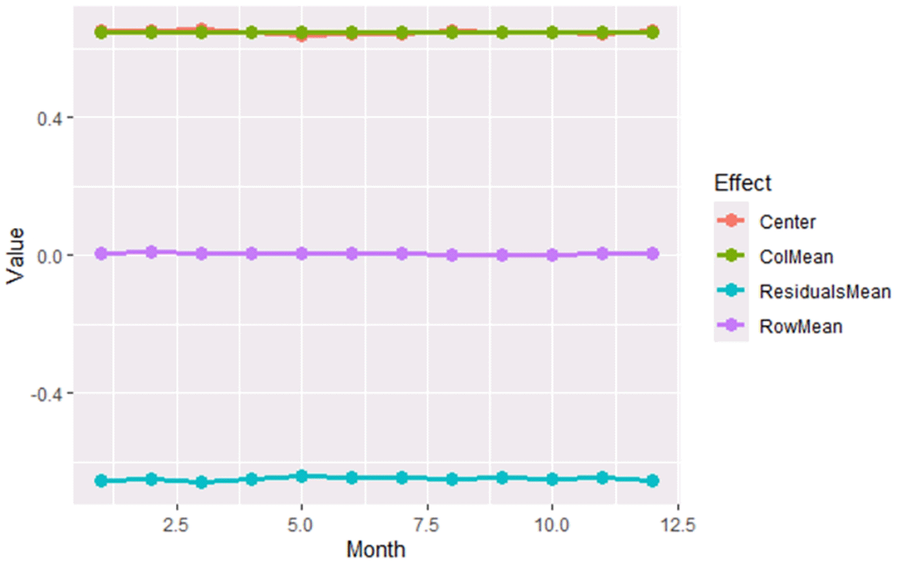
The figure shows the mean of the principal components resulting from the Two-Way Functional Median Polish. The central curve appears to be constant across months, while the row and column effects are close to zero, reflecting weak annual and seasonal variations. The average of the residuals is centered around zero on the functional scale, indicating limited unexplained variation.
Seventh: Perform ANOVA for the effects with plots after ANOVA analysis
-ANOVA function
run_anova <- function (effect_matrix, label) {
  df <- as.data.frame (effect_matrix)
  n <- nrow (df
)
  p <- ncol (df
)
  Year <- rep(1:n, times = p)
  Month <- factor (rep (colnames (df
), each = n))
  Value <- as.vector (as.matrix (df
))
  long_df <- data.frame (Year = factor (Year), Month = Month, Value = Value)
  result <- summary (aov (Value ~ Month, data = long_df
))
  pval <- result[[1]]$‘Pr(>F)’[1]
  cat("\n📊 ANOVA -", label, "|p-value =", round (pval, 4), "\n")
  return (pval)}
P-Value for effects
p_row1way <- run_anova(roweffect_oneway$data,"One way Row effects")
p_row2way <- run_anova(row2way, "Two way Row effects")
p_col2way <- run_anova(col2way, "Two way Column effects")
p_res2way <- run_anova(resid2way, "Two way Residuals")
The results and Plots
ANOVA_results <- data.frame (effects0 = c("Row (One-Way)", "Row (Two-Way)", "Column (Two-Way)", "Residual (Two-Way)"),
  p_value = c(p_row1way, p_row2way, p_col2way, p_res2way)
ANOVA_results$Significant <- ifelse (ANOVA_results$p_value < 0.05, "Significant", "Not Significant")
ggplot (ANOVA_results, aes(x = effects0, y = p_value, fill = Significant)) +
  geom_bar(stat = "identity", width = 0.5) +
  geom_hline(yintercept = 0.05, color = "red", linetype = "dashed", linewidth = 1) +

scale_fill_manual(values = c("Significant" = "gray", "Not Significant" = "black")) +
  labs (title = "ANOVA p-values for Functional Effects",
x = "components", y = "p-value", fill = "Significant") +
  theme_minimal(base_size = 14) +
  theme(axis.text.x = element_text(angle = 15, hjust = 0.8),

plot.title = element_text(hjust = 0.6))
The Figure 15 explain Residuals with IQR Band.
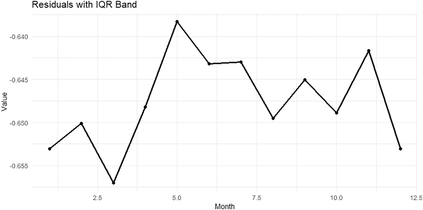
This figure displays the average residuals across months along with the interquartile range (IQR). We notice that the residuals are concentrated in the negative range (around zero with slight dispersion), with significant fluctuations between months. Some months (such as July and August) show residuals closer to zero (less negative), while in other months, such as February, June, and October, the residuals are more negative. This suggests that the model did not fully explain all monthly variations, and that some unexplained variances remain, reflecting the possibility of seasonal components or nonlinear effects that were not captured. While Figure 16 shows the ANOVA p-values for Functional Effects.
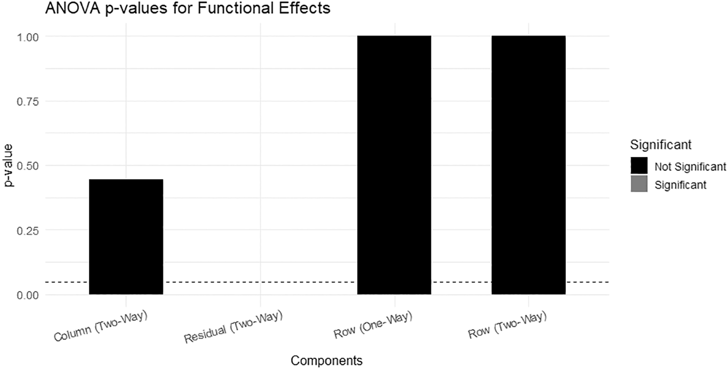
The bar chart shows the results of the ANOVA test for the FMP components.
• The row effects of years in both the one- and two-way models are not statistically significant (p ≈ 1). This means that the differences between years are not significant.
• The column effects of months showed a p-value of ≈ 0.45, which is also not statistically significant.
• The residuals are also insignificant.
This result means that most of the variation in the data cannot be clearly explained by effects of years or months alone, and that other dynamics (such as economic shocks or external factors) may be responsible for the changes.
This figure shows a comparison of the averages for the principal components:
• The red curve Center is stable around 0.64–0.65 on the functional scale.
• The green curve (ColMean) is almost constant, which confirms that the effect of months is almost constant and does not add additional explanation.
• The purple curve (RowMean) moves between approximately 1 and 3, meaning that the effect of years is very weak compared to the rest of the components.
• The blue curve (ResidualsMean) is clearly negative, meaning that the residuals account for most of the remaining variance not explained by the model.
• While Figure 17 shows Center vs Row/Column/Residual Means.
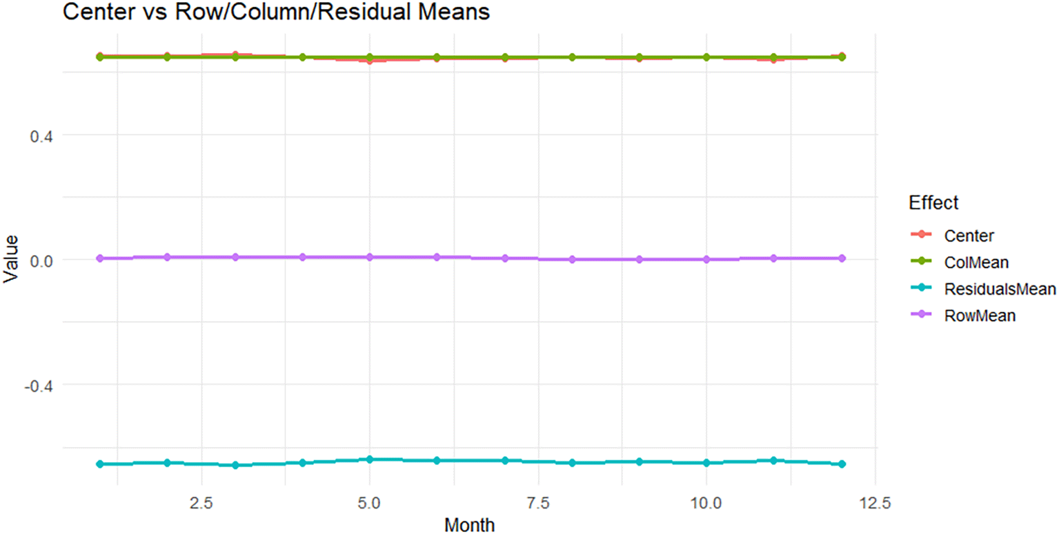
This figure confirms that the most important component captured by the model was the center (trend), while the rest of the components (annual and monthly) were weak and ineffective.
The figures show that:
1. The center represents the strongest structure in the data and is relatively constant around a value of 12.
2. The annual effects (Row effects) are very weak and do not reflect significant statistical differences between years.
3. The monthly effects (column effects(are approximately constant and statistically insignificant, meaning there is no clear seasonal pattern.
4. Residuals account for most of the variance, are biased toward negative values, and exhibit a non-normal distribution.
5. ANOVA test confirmed these results, as none of the components (except center) showed statistical significance.
The lack of seasonal significance in FANOVA can be attributed to factors such as the exchange rate regime, monetary operations, and monthly volatility. Furthermore, the jumps reflect shocks or news rather than a consistent monthly pattern. Purchase and shipping orders are spread over several months, weakening seasonal signals. That is, the short-term seasonal pattern disappears before it becomes statistically significant.
The results showed that the Fourier-based functional representation followed by the application of a one- and two-way FMP successfully extracted the center of the series and stabilized it around 0.64–0.65 on the functional scale, with a clear separation between the year and month components. FANOVA tests did not show monthly seasonal significance, and class effects were limited after functional transformation. The residuals were centered around zero with heavier tails at the extremities, indicating a good fit at the core, with tail skewness that can be addressed with heavier-tailed models. The study’s contributions are an integrated and anomaly-resistant path to transforming the monthly series into a uniform functional space over the range 1–12, followed by the application of a one- and two-way FMP, and linking the results to FANOVA tests and standard visual diagnostics. The most significant limitations remain the adoption of non-inflation-adjusted nominal prices, the absence of institutional explanatory variables, the univariate nature of the analysis, and the failure to explicitly model heavy tails. The results suggest introducing institutional and financing variables, moving to FPCA or multivariate models linking formal and parallel, documenting uncertainty through bootstrap procedures, and assessing out-of-sample predictive power.
| Views | Downloads | |
|---|---|---|
| F1000Research | - | - |
|
PubMed Central
Data from PMC are received and updated monthly.
|
- | - |
Provide sufficient details of any financial or non-financial competing interests to enable users to assess whether your comments might lead a reasonable person to question your impartiality. Consider the following examples, but note that this is not an exhaustive list:
Sign up for content alerts and receive a weekly or monthly email with all newly published articles
Already registered? Sign in
The email address should be the one you originally registered with F1000.
You registered with F1000 via Google, so we cannot reset your password.
To sign in, please click here.
If you still need help with your Google account password, please click here.
You registered with F1000 via Facebook, so we cannot reset your password.
To sign in, please click here.
If you still need help with your Facebook account password, please click here.
If your email address is registered with us, we will email you instructions to reset your password.
If you think you should have received this email but it has not arrived, please check your spam filters and/or contact for further assistance.
Comments on this article Comments (0)