Linear Shooting with High-Order Diagonally Implicit Runge-Kutta-Nystr&ouml;m Methods for Types of Second-Order Linear Boundary Value Problems with Applications

ibrahim abdullah muhammed; Firas Adel Fawzi

doi:10.12688/f1000research.172511.1

Home Browse Linear Shooting with High-Order Diagonally Implicit Runge-Kutta-Nyström...

ALL Metrics

-

Views

-

Downloads

Get PDF

Get XML

Export

▬

✚

Research Article

Linear Shooting with High-Order Diagonally Implicit Runge-Kutta-Nyström Methods for Types of Second-Order Linear Boundary Value Problems with Applications

[version 1; peer review: awaiting peer review]

ibrahim abdullah muhammed ¹, Firas Adel Fawzi¹

PUBLISHED 20 Jan 2026

Author details Author details

¹ Mathematics, Tikrit University, Tikrit, Saladin Governorate, Iraq

ibrahim abdullah muhammed
Roles: Conceptualization, Data Curation, Formal Analysis, Funding Acquisition, Investigation, Methodology, Project Administration, Resources, Software, Validation, Visualization, Writing – Original Draft Preparation, Writing – Review & Editing

Firas Adel Fawzi
Roles: Supervision

OPEN PEER REVIEW

REVIEWER STATUS AWAITING PEER REVIEW

This article is included in the Fallujah Multidisciplinary Science and Innovation gateway.

Abstract

Background

Second-order linear boundary value problems arise in many applications of science and engineering and are commonly treated by reducing them to first-order systems, which increases the computational cost. Direct high-order methods that preserve the second-order structure are therefore of interest.

Methods

This study proposes fixed-step, high-order diagonally implicit Runge–Kutta–Nyström (DIRKN) methods for the direct numerical solution of special second-order linear boundary value problems. Two schemes, DIRKN(3,4) and DIRKN(4,5), are constructed and combined with a linear shooting technique to handle both Dirichlet and Neumann boundary conditions without transforming the problem into a first-order system.

Results

The performance of the proposed methods is evaluated using benchmark test problems and application models, including rod heat conduction and reaction–diffusion equations. Numerical results demonstrate that both schemes achieve high accuracy and good efficiency, with DIRKN(4,5) generally producing smaller errors for a comparable number of function evaluations. A linear stability analysis shows absolute stability intervals of (−1.96, 0) for DIRKN(3,4) and (−7.24, 0) for DIRKN(4,5).

Conclusions

The proposed DIRKN methods provide accurate and efficient solvers for second-order linear boundary value problems with different types of boundary conditions, while preserving the original problem structure and reducing computational cost.

Keywords

Boundary Value Problem, Dirichlet boundary conditions, Neumann boundary conditions, Absolutely stability, Diagonally Implicit Runge-Kutta Nyström (DIRKN), Linear Shooting Technique, Second-Order Ordinary Differential Equation.

Corresponding author: ibrahim abdullah muhammed

Competing interests: No competing interests were disclosed.

Grant information: The author(s) declared that no grants were involved in supporting this work.

Copyright: © 2026 abdullah muhammed i and Adel Fawzi F. This is an open access article distributed under the terms of the Creative Commons Attribution License, which permits unrestricted use, distribution, and reproduction in any medium, provided the original work is properly cited.

How to cite: abdullah muhammed i and Adel Fawzi F. Linear Shooting with High-Order Diagonally Implicit Runge-Kutta-Nyström Methods for Types of Second-Order Linear Boundary Value Problems with Applications [version 1; peer review: awaiting peer review]. F1000Research 2026, 15:95 (https://doi.org/10.12688/f1000research.172511.1) First published: 20 Jan 2026, 15:95 (https://doi.org/10.12688/f1000research.172511.1) Latest published: 20 Jan 2026, 15:95 (https://doi.org/10.12688/f1000research.172511.1)

1. Introduction

Numerous methodologies have been developed to numerically address the two-point BVPs associated with special second order ODEs that take the following form:

(1)

y^{''} = f (x, y) where a \leq x \leq b

where

y \in ℝ^{d},

and

f : ℝ \times ℝ^{d} \to ℝ^{d}

are assumed to be sufficiently differentiable.

With boundary conditions:

(a) Type I: (Dirichlet boundary conditions)

(2)

y (a) = α, y (b) = β_{1}

(b) Type II: (Neumann boundary conditions)

(3)

y (a) = a, y^{'} (b) = β_{2}

Where $a, b, α, β_{1}, β_{2}$ are real numbers

One type of special second order ODEs (1) is a linear which have the from:

(4)

y^{''} = g (x) y + r (x)

Where $g (x), r (x)$ are continuous functions on the interval $[a, b]$ .

Two-point boundary value problems are prevalent in various applications, including the modeling of chemical reactions, boundary layer theory pertinent to fluid mechanics, and theories associated with heat transfer, among others. These problems can be articulated through various forms of boundary conditions, such as Dirichlet, Neumann, or mixed types, contingent on the defined boundary conditions. The Dirichlet boundary condition, recognized as the most extensively employed, has been examined by several researchers, including Hamid et al.¹ and Mohamad.² Furthermore, Liu³ investigates the Neumann-type boundary value problems.

The shooting method is employed to transform the BVP into two IVPs, where the shooting method is defined to find up the missing initial value, condition until the argument boundary conditions with respect to the other end reaches it’s valid values.¹⁷ Shooting method has been employed by Ha⁴ to solve BVPs. A two-point BVP has been studied in various applied fields. For solving numerically such problems, shooting methods^5,6,18 are the most popular. Shooting methods are useful in that it enjoys advantages like fast solver and small system size; however, it is time-consuming in obtaining a reasonable approximation, especially for nonlinear problems.⁷

The class of DIRKN methods has been extensively studied in the context of initial value problems (IVPs). For example, Sommeijer,¹⁹ Van der Houwen et al.,²⁰ Imoni et al.,¹⁴ Sharp et al.,²¹ Senu et al.,¹⁵ Papageorgiou et al.,²² and Medvedev et al.²³ developed and analyzed various DIRKN schemes for IVPs, while explicit RKN approaches were considered by Zanariah Abdul Majid et al.¹⁸ In fact, a substantial body of literature focuses on DIRKN methods for IVPs (see, e.g.,^11–13). However, their direct application to boundary value problems (BVPs) has received far less attention. In most studies, second-order BVPs are first transformed into equivalent first-order systems before applying numerical schemes, which increases the system size and may obscure the physical meaning of the variables.

To address this gap, one of the main objectives of this paper is to construct new high-order DIRKN schemes that solve Equation (1) directly in its second-order form under the boundary conditions (2)–(3), without conversion to a first-order system. This approach not only reduces computational cost but also preserves the structure of the original problem. Here we highlight the major contributions and findings of this article as follows:

• Derivation of high-order DIRKN schemes: construction of DIRKN(3,4) (third-stage, fourth-order) and DIRKN(4,5) (fourth-stage, fifth-order) with coefficients chosen to satisfy the order conditions and minimize the leading global truncation error.
• Use of linear shooting to handle boundary conditions (2)–(3) in the native second-order form.
• Absolute-stability analysis of the proposed DIRKN schemes.
• Implementation the proposed methods in applications.

To achieve the above objectives, in Sections 2 and 3, the materials and methods are addressed, respectively. Section 4 presents the numerical results, while the final section 5 provides a discussion and conclusions drawn from the study.

2. Materials

2.1 Diagonally implicit Runge-Kutta-Nyström (DIRKN)

The RKN method, originally proposed by Nyström (1925), is a class of methods for solving second-order IVPs. The diagonally implicit version (DIRKN) is particularly attractive due to its efficiency and stability, and its coefficients are commonly represented in a Butcher tableau ( Table 1).

Table 1. Butcher table of DIRKN.

$c_{1}$	$a_{11}$
$c_{2}$	$a_{21}$	$a_{22}$
$⋮$	$⋮$	$⋮$	$⋱$
$c_{m}$	$a_{m, 1}$	$a_{m, 2}$		$a_{mm}$
	$b_{1}$	$b_{2}$	$\dots$	$b_{m}$
	$b_{1}^{'}$	$b_{2}^{'}$	$\dots$	$b_{m}^{'}$

The DIRKN scheme tailored for special second-order IVPs is outlined as follows:

(5a)

y_{n + 1} = y_{n} + {hy}_{n}^{'} + h^{2} \sum_{i = 1}^{m} b_{i} k_{i}

(5b)

y_{n + 1}^{'} = y_{n}^{'} + h \sum_{i = 1}^{m} b_{i}^{'} k_{i}

Where

(6)

k_{i} = f (x_{n} + c_{i} h, y_{n} + c_{i} {hy}_{n}^{'} + h^{2} \sum_{j = 1}^{i} a_{ij} k_{j}) i = 1 ., \dots, m .

m is the number of stages and the parameters $a_{ij}, b_{j}, b^{'}, c_{j}$ are the coefficients of the method such that $c = {[c_{1}, c_{2}, \dots ., c_{m}]}^{T}, b = {[b_{1}, b_{2}, \dots, b_{m}]}^{T} b^{'} = {[b_{1}^{'}, b_{2}^{'}, \dots, b_{m}^{'}]}^{T}, A = {[a_{ij}]}_{m \times m}$ , and in DIRKN coefficients $a_{ij} = 0, for j > i$ and all entries of A are equal.¹⁶

2.2 The algebraic order conditions of Runge-Kutta-Nyström(RKN) method

The order conditions of an m-stage RKN method up to the six orders were introduced in reference⁹ as follows:

for $i = 1, 2, \dots, m and j = 1, 2, \dots, m$

The order conditions for y:

(7)

order 2 : \sum b_{i} = \frac{1}{2}

(8)

order 3 : \sum b_{i} c_{i} = \frac{1}{6}

(9)

order 4 : \frac{1}{2} \sum b_{i} c_{i}^{2} = \frac{1}{24}

(10)

order 5 : \frac{1}{6} \sum b_{i} c_{i}^{3} = \frac{1}{120}

(11)

\sum b_{i} a_{ij} c_{j} = \frac{1}{24}

(12)

Order 6 : \frac{1}{24} \sum b_{i} c_{i}^{4} = \frac{1}{720}

(13)

\frac{1}{4} \sum b_{i} c_{i} a_{ij} c_{j} = \frac{1}{720}

(14)

\frac{1}{2} \sum b_{i} a_{ij} {c_{j}}^{2} = \frac{1}{720}

The order conditions for $y^{'}$ :

(15)

order 1 : \sum b_{i}^{'} = 1

(16)

Order 2 : \sum b_{i}^{'} c_{i} = \frac{1}{2}

(17)

Order 3 : \frac{1}{2} \sum b_{i}^{'} c_{i}^{2} = \frac{1}{6}

(18)

Order 4 : \frac{1}{6} \sum b_{i}^{'} c_{i}^{3} = \frac{1}{24}

(19)

\sum b_{i}^{'} a_{ij} c_{j} = \frac{1}{24}

(20)

Order 5 : \frac{1}{24} \sum b_{i}^{'} c_{i}^{4} = \frac{1}{120}

(21)

\frac{1}{4} \sum b_{i}^{'} c_{i} a_{ij} c_{j} = \frac{1}{120}

(22)

\frac{1}{2} \sum b_{i}^{'} a_{ij} c_{i}^{2} = \frac{1}{120}

(23)

Order 6 : \frac{1}{120} \sum b_{i}^{'} c_{i}^{5} = \frac{1}{720}

(24)

\frac{1}{20} \sum b_{i}^{'} {c_{i}}^{2} a_{ij} c_{j} = \frac{1}{720}

(25)

\frac{1}{10} \sum b_{i}^{'} c_{i} a_{ij} {c_{j}}^{2} = \frac{1}{720}

(26)

\frac{1}{6} \sum b_{i}^{'} a_{ij} {c_{j}}^{3} = \frac{1}{720}

(27)

\sum b_{i}^{'} a_{ij} a_{jk} c_{k} = \frac{1}{720}

2.3 Shooting method for BVPs

Shooting method works in three steps⁸:

1. The given BVP is transformed in two IVPs in the same order.
2. Solution of these two IVPs can be found by any technique.
3. The solution to the given boundary value problem can be expressed as a linear combination of the two solutions provided.

Let $ψ (x)$ represent the singular solution to the IVP¹⁰:

(28)

ψ^{''} = f_{1} (x, ψ) = g (x) ψ (x) + r (x), with ψ (a) = α, ψ^{'} (a) = 0

(Non-homogeneous IVP)

Let $u (x)$ as the singular solution to the IVP:

(29)

u^{''} = f_{2} (x, u) = g (x) u (x), with u (a) = 0, u^{'} (a) = 1

(Homogeneous IVP).

Then the linear combination

(30)

y (x) = C_{1} ψ (x) + C_{2} u (x) .

represents a resolution to the linear BVP (4)

By setting C₁ = 1, the resultant solution y(t) in Equation (30) aligns with the specified boundary conditions.

Either, boundary condition Type I (2) the linear combination

(31)

y (a) = ψ (a) + C_{2} u (a), y (a) = α, y (b) = ψ (b) + C_{2} u (b) .

Imposing the boundary condition $y (b) = β_{1}$ in (31) produces $C_{2} = \frac{β_{1} - ψ (b)}{u (b)}$

Therefore, if $u (b) \neq 0$ , the distinct solution for the boundary value problem (1) which expressed by:

(32)

y (x) = ψ (x) + \frac{(β_{1} - ψ (b))}{u (b)} u (x)

Or, for boundary condition Type II the linear combination

(33)

y (a) = ψ (a) + C_{2} u (a), y (a) = α, y^{'} (b) = ψ^{'} (b) + C_{2} u^{'} (b)

Therefore, if $u^{'} (b) \neq 0$ , the distinct solution for the boundary value problem (1) which expressed by:

(34)

y^{'} (x) = ψ^{'} (x) + \frac{(β_{1} - ψ^{'} (b))}{u^{' (b)}} u^{'} (x)

2.4 Absolutely stability of DIRKN method

In studying the linear stability of DIRKN methods, we apply the scalar test equation

(35)

y^{''} = - λ^{2} y, λ \in R

in (5a), (5b) and (6), we obtain:

(36)

y_{n + 1} = y_{n} + {hy}_{n}^{'} + h^{2} \sum_{i = 1}^{m} b_{i} (- λ^{2} y_{n})

(37)

y_{n + 1}^{'} = y_{n}^{'} + h \sum_{i = 1}^{m} b_{i}^{'} (- λ^{2} y_{n})

(38)

k_{i} = f (x_{n} + c_{i} h, y_{n} + c_{i} {hy}_{n}^{'} + h^{2} \sum_{j = 1}^{i} a_{ij} (- λ^{2} y_{n}))

Setting $H = - {(h λ)}^{2}$ and multiplying (37) by $h$ , then (36) and (37) becomes:

(39)

y_{n + 1} = y_{n} + {hy}_{n}^{'} + H \sum_{i = 1}^{m} b_{i} y_{n}

(40)

h y_{n + 1}^{'} = h y_{n}^{'} + H \sum_{i = 1}^{m} b_{i}^{'} y_{n}

Therefore, we can write (39) and (40) by the form:

(\begin{matrix} y_{n + 1} \\ h y_{n + 1}^{'} \end{matrix}) = M (H) (\begin{matrix} y_{n} \\ {hy}_{n}^{'} \end{matrix})

where

M (H) = (\begin{matrix} 1 + H b^{T} L^{- 1} e & 1 + H b^{T} L^{- 1} c \\ Hb'^{T} L^{- 1} e & 1 + Hb'^{T} L^{- 1} c \end{matrix})

is the stability matrix and

(41)

L = I - HA, e = {(1, \dots, 1)}^{T}

Introducing the functions $S (H) = Trace (M) and p (H) = Det (M)$

Then the characteristic equation corresponding to the difference Equation (41) is of the form:

(42)

ξ^{2} - S (H) ξ + p (H) = 0

The roots $ξ_{1}$ and $ξ_{2}$ of (42) determine the behavior of the solution.

Definition 1

(Absolute-stability interval on the negative real axis)¹⁴: For a DIRKN method with stability matrix (41), an interval $(- H_{a}, 0)$ is called the absolute stability interval of the characteristic Equation (42) if, for all $H \in (- H_{a}, 0)$ we have $| ξ_{1, 2} | < 1$ , where $H_{a} > 0$ is the (largest) stability threshold on the negative real axis for the method.

3. Methods

3-1 Construction the new coefficients of third stage fourth order DIRKN(3,4)

In this subsection, the coefficients of DIRKN (3,4) are derived by using the order conditions up to fourth order for y and $y^{'}$ . As a result, a system of eight nonlinear equations with thirteen unknown variables is obtained. These equations are derived from the algebraic order conditions (7)–(9) and (15)–(19), by impose $a_{21} = 0, b_{3} = 0, b_{2}^{'} = 0$ and solve these equations by using solve command in Maple software, we get the values of $c_{1} = \frac{1}{2} - \frac{\sqrt{3}}{6}, c_{2} = \frac{1}{4} + \frac{\sqrt{3}}{12}, c_{3} = \frac{1}{2} + \frac{\sqrt{3}}{6}, b_{1} = \frac{1}{4} + \frac{\sqrt{3}}{12}, b_{2} = \frac{1}{4} + \frac{\sqrt{3}}{12}, b_{1}^{'} = \frac{1}{2}, b_{3}^{'} = \frac{1}{2}$ . According to Dormand,¹⁰ the free parameters $a_{31}, a_{32}$ are selected by minimizing the global truncation error for the fifth-order conditions of y and y′ by using Maple where:

(43)

{‖ τ_{g}^{(4)} ‖}_{2} = \sqrt{\sum_{i = 1}^{2} {(τ_{i}^{(4)})}^{2} + \sum_{i = 1}^{3} {({τ^{'}}_{i}^{(4)})}^{2}}

is the global truncation error and $τ_{i}^{(4)}$ , and ${τ^{'}}_{i}^{(4)}$ are the local truncation error terms which gives from the Equations (10)-(11) and (20)-(22) of the RKN method for y, and y’, respectively. We get:

(44)

τ_{1}^{(4)} = \frac{1}{6} \sum b_{i} c_{i}^{3} - \frac{1}{120}

(45)

τ_{2}^{(4)} = \sum b_{i} a_{ij} c_{j} - \frac{1}{24}

(46)

{τ^{'}}_{1}^{(4)} = \frac{1}{24} \sum b_{i}^{'} c_{i}^{4} - \frac{1}{120}

(47)

{τ^{'}}_{2}^{(4)} = \frac{1}{4} \sum b_{i}^{'} c_{i} a_{ij} c_{j} - \frac{1}{120}

(48)

{τ^{'}}_{3}^{(4)} = \frac{1}{2} \sum b_{i}^{'} a_{ij} c_{i}^{2} - \frac{1}{120}

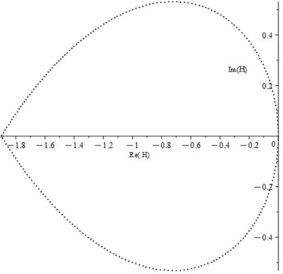
We obtained $a_{31} = 0.0307, a_{32} = - 0.0772 and {‖ τ_{g}^{(4)} ‖}_{2} = 2.72 E - 12$ . Lastly, all the coefficients of the DIRKN(3,4) are written in Table 2. The stability interval (which show in the subsection 2.4) of the new DIRKN(3,4) is approximately (−1.964,0) while the stability region show in Figure 1 show the of the proposed method in Im(H) - Re(H) plane is determined by substituting $ξ$ in the characteristic Equation (42) with 1, -1 and $e^{iθ}$ for $θϵ [0, 2 π]$ . The wider stability interval indicate that larger step sizes can be taken without loss of stability.

Table 2. coefficients of DIRKN(3,4).

0.211	0.12	0	0
0.789	0	0.12	0
0.789	0.0307	-0.0772	0.12
	0.394	0.106	0
	0.5	0	0.5

Figure 1. Stability region of the proposed DIRKN(3,4) method in the Im(H)–Re(H) plane, showing the absolute-stability domain on the negative real axis.

3-2 construction the new coefficients of fourth stage fifth order DIRKN (4,5)

In the same way, the coefficients of DIRKN (4,5) were derived, but fifth-order equations were used, which affects the number of variables and the number of equations. Thirteen nonlinear equations have obtained with nineteen unknown variables. By impose $c_{1} = 0, b_{2} = 0, b_{2}^{'} = 0,$ $a_{21} = 0$ and solve the Equations (7)-(11) and (15)-(22). The free parameters $a_{32}, a_{44}$ are selected by reducing the error in Equations (12)-(14) and (23)-(27). We get;

${‖ τ_{g}^{(4)} ‖}_{2} = 9.651 E - 16$ and all the coefficients of the DIRKN(4,5) are written in Table 3.

Table 3. Coefficients of DIRKN (4,5).

0	1	0	0	0
-0.970	0	1	0	0
0.845	-1.88	1	1	0
0.355	0.63	-0.736	-0.85	1
	0.111	0	0.058	0.330
	0.111	0	0.376	0.512

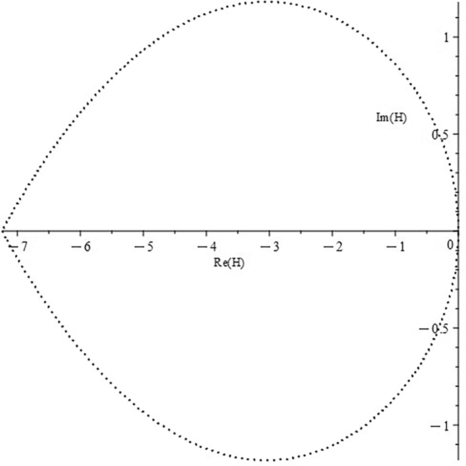
The stability interval of the new DIRKN(4,5) is approximately (−7.244,0) and Figure 2 show the stability region of the proposed method in Im(H) - Re(H) plane.

Figure 2. Stability region of the proposed DIRKN(4,5) method in the Im(H)–Re(H) plane, illustrating its wider stability interval compared with DIRKN(3,4).

3.3 Algorithm of linear shooting technique via DIRKN method

approximate solution BVP (1) with boundary conditions (2) or (3)

INPUT: Parameters α, β₁, β₂ boundary conditions; endpoints a, b; number of subintervals N; coefficients of suggestion DIRKN method the vectors b, $b^{'}$ , c, and the matrix A.

OUTPUT: Numerical solution $y (x_{i})$ at $x_{i} = a + ih$ for all $i = 0, 1 \dots N$

Step 1: Initialization

set $h = (b - a) / N$

Set $ψ^{(0)} = α, {ψ^{'}}^{(0)} = 0 (IVPs for ψ - problem)$

Set $u^{(0)} = 0, {u^{'}}^{(0)} = 1 (IVPs for u - problem)$

Step 2: Solve IVPs (28)- (29) via DIRKN (5a)- (6)

for $n = 0, \dots . N - 1$ do Step 3 and Step 4

Step 3: Set $x_{n} = a + nh$

For stages $i = 1, 2, \dots, m$

k_{i} = f 1 (x_{n} + c_{i} h, ψ^{(n)} + ci h {ψ^{'}}^{(n)} + h^{2} \sum_{j = 1}^{i} a_{ij} k_{j}), (for ψ - problem)

k_{i} - f 1 (x_{n} + c_{i} h, ψ^{(n)} + ci h {ψ^{'}}^{(n)} + h^{2} \sum_{j = 1}^{i} a_{ij} k_{j}) = 0

Use fsolve in Maple command to solve above implicit equation to find $k_{i}$

Updated solution

ψ^{(n + 1)} = ψ^{(n)} + h {ψ^{'}}^{(n)} + h^{2} \sum_{i = 1}^{m} b_{i} k_{i}

{ψ^{'}}^{(n + 1)} = {ψ^{'}}^{(n)} + h \sum_{i = 1}^{m} b_{i}^{'} k_{i}

L_{i} = f 2 (x_{n} + c_{i} h, u^{(n)} + ci h {u^{'}}^{(n)} + h^{2} \sum_{j = 1}^{i} a_{ij} L_{j}), (for u - problem)

L_{i} - f 2 (x_{n} + c_{i} h, u^{(n)} + c_{i} h {u^{'}}^{(n)} + h^{2} \sum_{j = 1}^{i} a_{ij} L_{j}) = 0

Use fsolve in Maple command to solve above implicit equation to find $L_{i}$

Updated solution

u^{(n + 1)} = u^{(n)} + h {u^{'}}^{(n)} + h^{2} \sum_{i = 1}^{m} b_{i} L_{i}

{u^{'}}^{(n + 1)} = {u^{'}}^{(n)} + h \sum_{i = 1}^{m} b_{i}^{'} L_{i}

Step 4: Apply Boundary Conditions

if Type I $(y (b) = β_{1})$

then $C = \frac{β_{1} - ψ^{(N)}}{u^{(N)}}$

if Type II $((y^{'} (b) = β_{2}))$

then $C = \frac{β_{2} - {ψ^{'}}^{(N)}}{{u^{'}}^{(N)}}$

Step 5: Output Solution

for $i = 1, \dots, N$

y (x_{i}) = ψ^{(i)} + C u^{(i)}

Output $(x_{i}, y (x_{i}))$

Step 6: The process is complete

4. Numerical results

In this part, a suggested DIRKN (3,4) and DIRKN (4,5) approaches was utilized to address ODEs (1) with (2) or (3) boundary conditions. The method had been applied on fourth problems, The first two problems are used conditions of Type I (2) and the last second problems are used conditions of Type II (3). For comparison purpose, the numerical results are compared by the function calls and maximum errors between exact and numerical solution measurements by a proposed methods with the three previous studies. The Tables 4 and 5 utilize the subsequent notations:

• h: Step size.
• N: Number of partitions of interval.
• FC: Number of function Call.
• Max.Error: Max $(| y (x_{n}) - y_{n} |)$ which the maximum absolute errors between exact solutions $y (x_{n})$ and proposed numerical solutions $y_{n}$ .
• DIRKN (3,4): 3-stage 4-order DIRKN which was proposed in this paper.
• DIRKN (4,5): 4-stage 5-order DIRKN which was proposed in this paper.
• RKN (3,4) H: The 3-stage 4-order RKN derived by Hairer et al.²¹
• RKN (3,4) G: The 3-stage 4-order was developed by Garcia et al.²²
• TSRKN(3,4)A: The 3-stage 4-order two-step explicit RKN method derived by Abdulsalam et al.²⁴

Problem 1:

(Application Problem – Rod Heat Conduction Model)²⁵:

Suppose a slender rod of length L, with the temperature at the location x = 0 fixed at $t_{0}$ , while the opposite end at x = L is thermally insulated. It is assumed that the rod possesses a cross-sectional area that remains constant and is denoted as M, and that its perimeter is represented by p. The temperature u of the rod at a generic position x within the interval (0, L) is expressed as:

- {δMy}^{''} (x) + γpy (x) = 0, 0 \leq x \leq L

Type II : y (0) = y_{0}, y^{'} (L) = 0

where

δ

represents the thermal conductivity and

γ

signifies the convective transfer coefficients.

Exact solution: $y (x) = y_{0} \frac{cosh (μ (L - x))}{cosh (μL)}$ where $μ = \sqrt{\frac{γp}{δM}}$ and assume that the rod’s length is L = 100 cm and that the rod has a circular cross-section of radius 2 cm (and thus, M = 4π ${cm}^{2}$ , p = 4π cm). Also set $y_{0} = 10^{o}$ C $, γ = 2$ and $δ = 200$ .

Problem 2:

(Application Problem - the Reaction-Diffusion Model)²⁶:

Consider a homogeneous one-dimensional medium of length L = 1, where y(x) denotes the steady concentration (or temperature) at position $x \in (0, 1)$ . The process includes linear diffusion together with a constant reaction rate $k = 10^{- 2}$

y^{''} (x) - ky (x) = 0, 0 \leq x \leq 1

Type II : y (0) = 1, y^{'} (1) = 0

Exact solution: $y (x) = \frac{cosh \sqrt{k} (1 - x)}{cosh \sqrt{k}}$

Problem 3:

Homogonous linear BVPs¹:

y^{''} (x) = y (x), 0 \leq x \leq 1

Type I : y (0) = 1, y (1) = sinh (1)

exact solution : y (x) = sinh (x)

Problem 4:

Non homogonous linear BVPs of type I¹:

y^{''} (x) = π^{2} y (x) - 2 π^{2} sin (πt), 0 \leq x \leq 1

Type I : y (0) = 0, y (1) = 0

exact solution : y (x) = sin (πx)

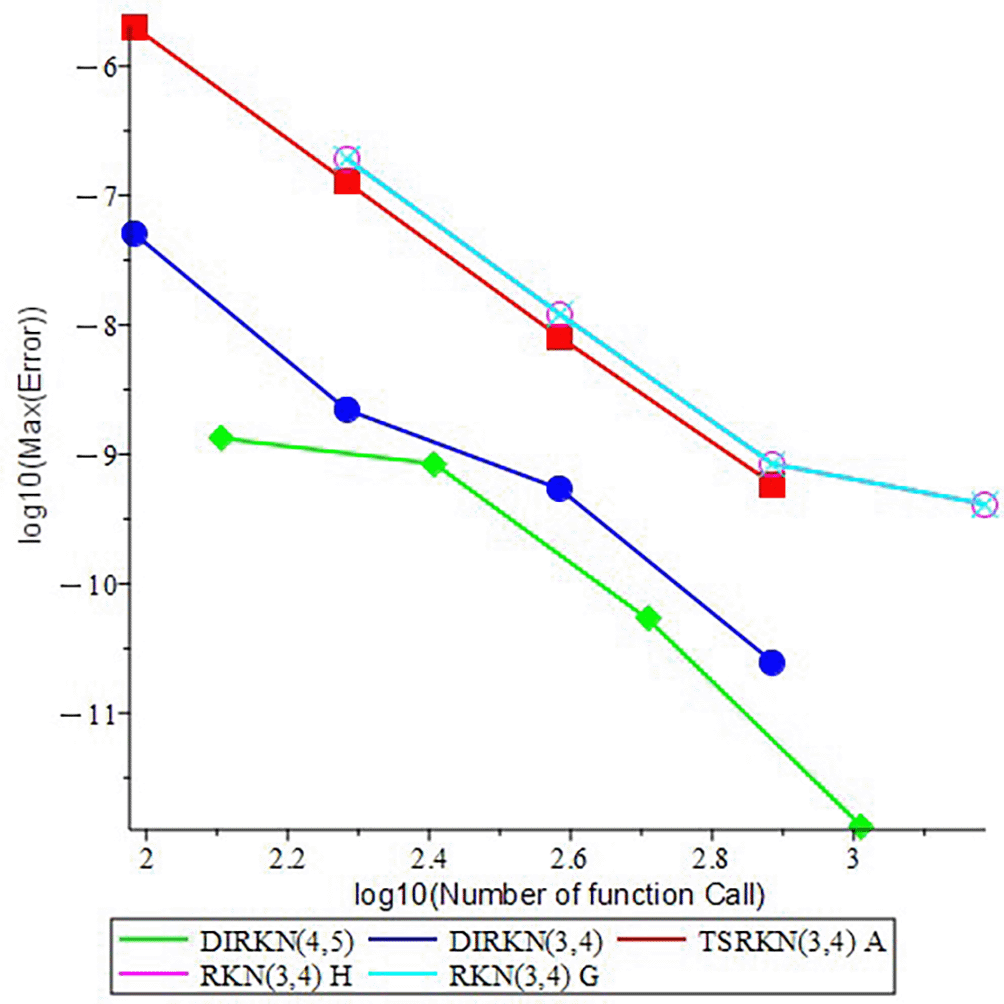
To further illustrate the effectiveness and performance of the proposed methodologies, we present the efficiency curves for DIRKN(3,4) and DIRKN(4,5) in comparison other established methods.

Figures 3-6 display the efficiency curves corresponding to the problems (1)-(4) that have been analyzed, respectively.

Table 4. Numerical results for problems (1-2) of type II by DIRKN (3,4), DIRKN (4,5), TSRKN (3,4) A, RKN (3,4) H and RKN (3,4) G.

				Problem 1	Problem 2
h	Methods	N	FC	Max.Error	Max.Error
$\frac{1}{16}$	DIRKN (4,5)	16	64	5.434133921E-6	3.325147428E-16
	DIRKN (3,4)	16	48	9.541189082E-5	7.141147376E-15
	TSRKN (3,4) A	8	48	2.020450902E-2	3.794742298E-13
	RKN (3,4) H	16	96	2.380008876E-3	4.873879078E-14
	RKN (3,4) G	16	96	1.114941947E-3	2.375877273E-14
$\frac{1}{32}$	DIRKN (4,5)	32	128	2.921766035E-7	5.412652302E-17
	DIRKN (3,4)	32	96	6.765139914E-6	9.211274038E-16
	TSRKN (3,4) A	16	96	9.999666680E-4	2.298161661E-14
	RKN (3,4) H	32	192	1.296792552E-4	3.330669074E-15
	RKN (3,4) G	32	192	6.268651822E-5	1.887379142E-15
$\frac{1}{64}$	DIRKN (4,5)	64	256	1.447574317E-8	5.311283226E-18
	DIRKN (3,4)	64	192	4.721394564E-7	7.410423124E-17
	TSRKN (3,4) A	32	192	5.659636107E-5	1.110223025E-15
	RKN (3,4) H	64	384	7.451809623E-6	1.110223025E-15
	RKN (3,4) G	64	384	3.662572766E-6	1.776356839E-15
$\frac{1}{128}$	DIRKN (4,5)	128	512	2.732977968E-9	4.731756164E-19
	DIRKN (3,4)	128	384	4.551997353E-8	8.281384293E-18
	TSRKN (3,4) A	64	384	3.318097021E-6	6.661338148E-16
	RKN (3,4) H	128	768	4.471133135E-7	8.881784197E-16
	RKN (3,4) G	128	768	2.216358665E-7	3.774758284E-15

Table 5. Numerical results for problems (3-4) of type I by DIRKN (3,4), DIRKN (4,5), TSRKN (3,4) A, RKN (3,4) H and RKN (3,4) G.

				Problem 3	Problem 4
h	Methods	N	FC	Max.Error	Max.Error
$\frac{1}{32}$	DIRKN (4,5)	32	128	1.453315132E-12	1.328196428E-9
	DIRKN (3,4)	32	96	3.949695961E-11	5.141147376E-8
	TSRKN (3,4) A	16	96	2.546295619E-9	2.039230214E-6
	RKN (3,4) H	32	192	3.584967878E-10	1.939488554E-7
	RKN (3,4) G	32	192	1.805622318E-10	1.934506531E-7
$\frac{1}{64}$	DIRKN (4,5)	64	256	6. 652652135E-13	8.416152302E-10
	DIRKN (3,4)	64	192	9.211277428E-12	2.21318038E-9
	TSRKN (3,4) A	32	192	1.643867265E-10	1.276113937E-7
	RKN (3,4) H	64	384	2.281685951E-11	1.218284962E-8
	RKN (3,4) G	64	384	1.145028516E-11	1.217505874E-8
$\frac{1}{128}$	DIRKN (4,5)	128	512	3.314373226E-14	5.311271226E-11
	DIRKN (3,4)	128	384	5.410423124E-13	5.410423124E-10
	TSRKN (3,4) A	64	384	1.041688957E-11	8.053617329E-9
	RKN (3,4) H	128	768	1.438293928E-12	8.437114341E-10
	RKN (3,4) G	128	768	7.210898545E-13	8.441253252E-10
$\frac{1}{256}$	DIRKN (4,5)	256	1024	5.731851164E-15	1.341789164E-12
	DIRKN (3,4)	256	768	8.281394293E-14	2.481384293E-11
	TSRKN (3,4) A	128	768	6.550315845E-13	5.902431877E-10
	RKN (3,4) H	256	1536	9.003908730E-14	4.102065829E-10
	RKN (3,4) G	256	1536	4.640732243E-14	4.102070444E-10

Figure 3. Efficiency curve for Problem 1 (Rod Heat Conduction Model): comparison of Max.Error versus function calls for DIRKN(3,4), DIRKN(4,5), and reference methods.

Figure 4. Efficiency curve for Problem 2 (Reaction–Diffusion Model): comparison of Max.Error versus function calls for DIRKN(3,4), DIRKN(4,5), and reference methods.

Figure 5. Efficiency curve for Problem 3 (Homogeneous Linear BVP): performance comparison between DIRKN schemes and benchmark RKN/TSRKN methods.

5. Discussion and conclusion

5.1 Discussion of results

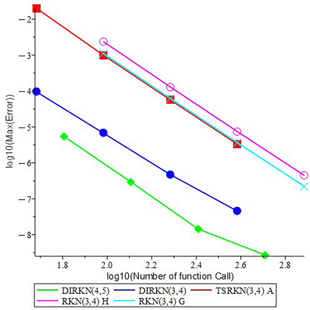
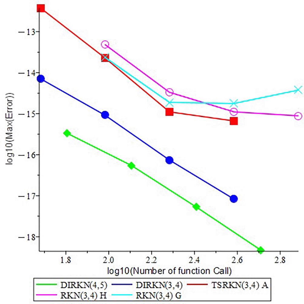
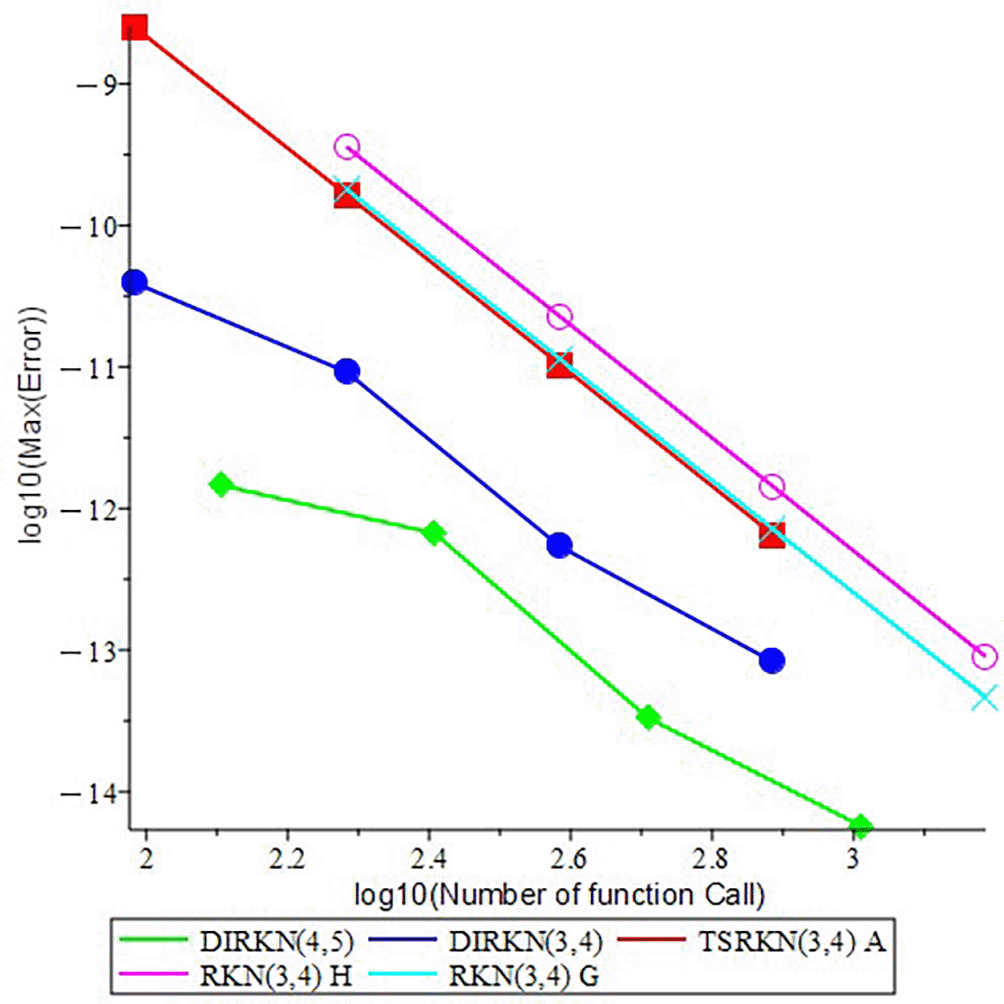
• Accuracy of numerical results. For all Type I (problems 1-2) and Type II (problems 3-4) problems, both methods, DIRKN(3,4) and DIRKN(4,5), produce very small maximum errors (Max.Error). At the same number of partitions of interval N, DIRKN(4,5) is usually more accurate than DIRKN(3,4) and both is more accurate than TSRKN (3,4) A, RKN (3,4) H and RKN (3,4) G but TSRKN (3,4) A have a small N because it two step method.
• Efficiency (error vs. cost). Efficiency plots (Max.Error vs. FC in Figures 3-6) show that DIRKN(4,5) needs fewer function calls to reach a given accuracy than the reference. As the accuracy demand increases (smaller Max.Error), the gap becomes larger. Thus, DIRKN(3,4) and DIRKN(4,5) offers a better accuracy cost trade off.
• Linear stability and its impact. The absolute stability interval on the negative real axis is wider for DIRKN(4,5) than for DIRKN(3,4) ((-7.24, 0) vs. (-1.96, 0)). This helps in problems with oscillation or stiffness: we can take a larger step h while staying stable, so we keep accuracy with less cost. This agrees with the efficiency results.
• Robustness for both boundary types and application models. On application models heat conduction in a rod (problem 1) and reaction–diffusion (problem 2), the methods preserve high accuracy under Type II conditions and match the exact solutions closely. Solving the BVP in its second-order form (without converting to a first-order system) keeps the physical structure and reduces the system size.
• Shooting strategy. The experiments use linear shooting because the problems are linear. This approach is simple and effective. Parallel shooting methods were not employed since all test problems are linear and can be efficiently solved using linear shooting. However, extending the proposed DIRKN schemes with parallel shooting will be an interesting direction for future research, particularly for nonlinear or stiff problems.

Figure 6. Efficiency curve for Problem 4 (Nonhomogeneous Linear BVP): accuracy–cost relationship among DIRKN(3,4), DIRKN(4,5), and reference solvers.

5.2 Conclusions

We constructed DIRKN(3,4) and DIRKN(4,5) schemes for second-order linear BVPs and chose coefficients to satisfy the order conditions and reduce the leading global truncation error. On Type I and Type II tests, both methods show high accuracy and good stability. In most cases, DIRKN(4,5) gives the lowest Max.Error for the same N (or the same FC). The wider stability interval of DIRKN(4,5) explains its practical advantage on oscillatory or stiff problems: we can keep stability with larger h, which improves efficiency. Working directly with the second-order form avoids increasing the dimension and keeps a clear physical meaning of the variables. Overall, the proposed DIRKN methods are reliable and efficient tools for linear second-order BVPs with conditions (2) or (3).The present study was restricted to linear BVPs. Extending the proposed DIRKN methods to nonlinear problems will be considered in future work.

Ethics and consent

Ethics and consent were not necessary.

Data availability

All numerical results presented in this study are generated computationally using the developed Maple algorithms. Since the results are fully reproducible from the provided implementation, no separate datasets are required. The source code used to generate the results is openly available via Zenodo at: https://doi.org/10.5281/zenodo.18134040

Software availability

Source code available from: https://github.com/Ibra1993125/DIRKN-Linear-Shooting

Archived software available from: https://doi.org/10.5281/zenodo.18134040

License: MIT License

Extended data

No extended data are associated with this article.

Acknowledgements

The authors thank the editors and the anonymous reviewers for their valuable suggestions in improving this paper.

References

1. Abd Hamid NN, Majid AA, Ismail AIM: Extended cubic B-spline method for linear two-point boundary value problems. Sains Malaysiana. 2011; 40(11): 1285–1290.
2. Mohamad AJA: Solving second order non-linear boundary value problems by four numerical methods. Eng. Tech. J. 2010; 28(2): 369–381.
3. Liu Y: Studies on Neumann-type boundary value problems for second-order nonlinear p-Laplacian-like functional differential equations. Nonlinear Analysis: Real World Applications. 2009; 10(1): 333–344.
4. Ha SN: A nonlinear shooting method for two-point boundary value problems. Comput. Math. Appl. 2001; 42(10-11): 1411–1420.
5. Phana PS, Maiid ZA, Suleiman M, et al.: Solving Boundary Value Problems With Neumann Conditions Using Direct Method.2013.
6. Inç M, Evans DJ: The decomposition method for solving of a class of singular two-point boundary value problems. Int. J. Comput. Math. 2003; 80(7): 869–882.
7. Jang B: Two-point boundary value problems by the extended Adomian decomposition method. J. Comput. Appl. Math. 2008; 219(1): 253–262.
8. Adam B, Hashim MH: Shooting method in solving boundary value problem. International Journal of Research and Reviews in Applied Sciences. 2014; 21(1): 8.
9. Fehlberg E: Classical seventh-, sixth-, and fifth-order Runge-Kutta-Nystróm formulas with step size control for general second-order differential equations (No. NASA-TR-R-432).1974.
10. Dormand JR: Numerical methods for differential equations: a computational approach. CRC press; 2018.
11. Franco JM: Exponentially fitted explicit Runge–Kutta–Nyström methods. J. Comput. Appl. Math. 2004; 167(1): 1–19.
12. Fawzi FA, Ghawadri NG: Embedded Schemes of the Runge-Kutta Type for the Direct Solution of Fourth-Order Ordinary Differential Equations. Iraqi Journal for Computer Science and Mathematics. 2024; 5(4): 8.
13. Fawzi FA: An Embedded 5 (4) Pair of Optimized Runge-Kutta Method for the Numerical Solution of Periodic Initial Value Problems. Iraqi Journal of Science. 2022; 3889–3901.
14. Imoni SO, Otunta FO, Ramamohan TR: Embedded implicit Runge- Kutta- Nyström method for solving second-order differential equations. Int. J. Comput. Math. 2006; 83: 777–784.
15. Senu N, Suleiman MOHAMED, Ismail F, et al.: A new diagonally implicit Runge-Kutta-Nyström method for periodic IVPs. WSEAS Trans. Math. 2010; 9(9): 679–688.
16. Al-fayyadh KA, Fawzi FA, Hussain KA: Exponentially Fitted-Diagonally Implicit Runge-Kutta Method for Direct Solution of Fifth-Order Ordinary Differential Equations. Journal of Al-Qadisiyah for Computer Science and Mathematics. 2025; 17(1): 142–158.
17. Mechee MS, Fawzi FA, Abdullah SM: A numerical study of linear two-points boundary value problems with odes of fourth-order using RKM method. Academic Science Journal. 2025; 3(1): 65–78. Publisher Full Text
18. Majid ZA, Abdulsalam A, Senu N: Runge-Kutta-Nystrom Methods for Directly Solving Second Order Linear Boundary Value Problems with Dirichlet Condition. Emerging Themis in fundamental and applied science: mathematics. UPM Press; 2018; V. 1. , pp. 1–89.
19. Senu N, Suleiman M, Ismail F, et al.: A singly diagonally implicit Runge-Kutta-Nyström method for solving oscillatory problems. IAENG Int. J. Appl. Math. 2011; 41(2): 155–161.
20. Sharp PW, Fine JM, Burrage K: Two-stage and three-stage diagonally implicit Runge-Kutta Nyström methods of orders three and four. IMA J. Numer. Anal. 1990; 10(4): 489–504.
21. Hairer E, Wanner G, Nørsett SP: Solving ordinary differential equations I: Nonstiff problems. Berlin, Heidelberg: Springer Berlin Heidelberg; 1993.
22. Garcı́a A, Martı́n P, González AB: New methods for oscillatory problems based on classical codes. Appl. Numer. Math. 2002; 42(1-3): 141–157.
23. Lambert JD: Numerical methods for ordinary differential systems. New York: Wiley; 1991; vol. 146. .
24. Abdulsalam A, Senu N, Majid ZA: Two-step RKN direct method for special second-order initial and boundary value problems. IAENG Int. J. Appl. Math. 2021; 51(3): 1–9.
25. Quarteroni A, Sacco R, Saleri F: Numerical mathematics. Springer Science & Business Media; 2006; vol. 37. .
26. Na TY: Computational methods in engineering boundary value problems. Academic press; 1980; vol. 145. .

Comments on this article Comments (0)

Version 1

VERSION 1 PUBLISHED 20 Jan 2026

Author details Author details

¹ Mathematics, Tikrit University, Tikrit, Saladin Governorate, Iraq

ibrahim abdullah muhammed
Roles: Conceptualization, Data Curation, Formal Analysis, Funding Acquisition, Investigation, Methodology, Project Administration, Resources, Software, Validation, Visualization, Writing – Original Draft Preparation, Writing – Review & Editing

Firas Adel Fawzi
Roles: Supervision

Competing interests

No competing interests were disclosed.

Grant information

The author(s) declared that no grants were involved in supporting this work.

Article Versions (1)

version 1

Published: 20 Jan 2026, 15:95

https://doi.org/10.12688/f1000research.172511.1

Copyright

© 2026 abdullah muhammed i and Adel Fawzi F. This is an open access article distributed under the terms of the Creative Commons Attribution License, which permits unrestricted use, distribution, and reproduction in any medium, provided the original work is properly cited.

Download

Export To

metrics

	Views	Downloads
F1000Research	-	-
PubMed Central Data from PMC are received and updated monthly.	-	-

Citations

0

SEE MORE DETAILS

CITE

how to cite this article

abdullah muhammed i and Adel Fawzi F. Linear Shooting with High-Order Diagonally Implicit Runge-Kutta-Nyström Methods for Types of Second-Order Linear Boundary Value Problems with Applications [version 1; peer review: awaiting peer review]. F1000Research 2026, 15:95 (https://doi.org/10.12688/f1000research.172511.1)

NOTE: If applicable, it is important to ensure the information in square brackets after the title is included in all citations of this article.

track

receive updates on this article

Track an article to receive email alerts on any updates to this article.

Open Peer Review

Comments on this article Comments (0)

Version 1

VERSION 1 PUBLISHED 20 Jan 2026

Open Peer Review

Reviewer Status

AWAITING PEER REVIEW

Comments on this article

All Comments(0)

Add a comment

Sign up for content alerts

Browse by related subjects

[1] 1. Abd Hamid NN, Majid AA, Ismail AIM: Extended cubic B-spline method for linear two-point boundary value problems. Sains Malaysiana. 2011; 40(11): 1285–1290.

[2] 2. Mohamad AJA: Solving second order non-linear boundary value problems by four numerical methods. Eng. Tech. J. 2010; 28(2): 369–381.

[3] 3. Liu Y: Studies on Neumann-type boundary value problems for second-order nonlinear p-Laplacian-like functional differential equations. Nonlinear Analysis: Real World Applications. 2009; 10(1): 333–344.

[4] 4. Ha SN: A nonlinear shooting method for two-point boundary value problems. Comput. Math. Appl. 2001; 42(10-11): 1411–1420.

[5] 5. Phana PS, Maiid ZA, Suleiman M, et al.: Solving Boundary Value Problems With Neumann Conditions Using Direct Method.2013.

[6] 6. Inç M, Evans DJ: The decomposition method for solving of a class of singular two-point boundary value problems. Int. J. Comput. Math. 2003; 80(7): 869–882.

[7] 7. Jang B: Two-point boundary value problems by the extended Adomian decomposition method. J. Comput. Appl. Math. 2008; 219(1): 253–262.

[8] 8. Adam B, Hashim MH: Shooting method in solving boundary value problem. International Journal of Research and Reviews in Applied Sciences. 2014; 21(1): 8.

[9] 9. Fehlberg E: Classical seventh-, sixth-, and fifth-order Runge-Kutta-Nystróm formulas with step size control for general second-order differential equations (No. NASA-TR-R-432).1974.

[10] 10. Dormand JR: Numerical methods for differential equations: a computational approach. CRC press; 2018.

[11] 11. Franco JM: Exponentially fitted explicit Runge–Kutta–Nyström methods. J. Comput. Appl. Math. 2004; 167(1): 1–19.

[12] 12. Fawzi FA, Ghawadri NG: Embedded Schemes of the Runge-Kutta Type for the Direct Solution of Fourth-Order Ordinary Differential Equations. Iraqi Journal for Computer Science and Mathematics. 2024; 5(4): 8.

[13] 13. Fawzi FA: An Embedded 5 (4) Pair of Optimized Runge-Kutta Method for the Numerical Solution of Periodic Initial Value Problems. Iraqi Journal of Science. 2022; 3889–3901.

[14] 14. Imoni SO, Otunta FO, Ramamohan TR: Embedded implicit Runge- Kutta- Nyström method for solving second-order differential equations. Int. J. Comput. Math. 2006; 83: 777–784.

[15] 15. Senu N, Suleiman MOHAMED, Ismail F, et al.: A new diagonally implicit Runge-Kutta-Nyström method for periodic IVPs. WSEAS Trans. Math. 2010; 9(9): 679–688.

[16] 16. Al-fayyadh KA, Fawzi FA, Hussain KA: Exponentially Fitted-Diagonally Implicit Runge-Kutta Method for Direct Solution of Fifth-Order Ordinary Differential Equations. Journal of Al-Qadisiyah for Computer Science and Mathematics. 2025; 17(1): 142–158.

[17] 17. Mechee MS, Fawzi FA, Abdullah SM: A numerical study of linear two-points boundary value problems with odes of fourth-order using RKM method. Academic Science Journal. 2025; 3(1): 65–78. Publisher Full Text

[18] 18. Majid ZA, Abdulsalam A, Senu N: Runge-Kutta-Nystrom Methods for Directly Solving Second Order Linear Boundary Value Problems with Dirichlet Condition. Emerging Themis in fundamental and applied science: mathematics. UPM Press; 2018; V. 1. , pp. 1–89.

[19] 19. Senu N, Suleiman M, Ismail F, et al.: A singly diagonally implicit Runge-Kutta-Nyström method for solving oscillatory problems. IAENG Int. J. Appl. Math. 2011; 41(2): 155–161.

[20] 20. Sharp PW, Fine JM, Burrage K: Two-stage and three-stage diagonally implicit Runge-Kutta Nyström methods of orders three and four. IMA J. Numer. Anal. 1990; 10(4): 489–504.

[21] 21. Hairer E, Wanner G, Nørsett SP: Solving ordinary differential equations I: Nonstiff problems. Berlin, Heidelberg: Springer Berlin Heidelberg; 1993.

[22] 22. Garcı́a A, Martı́n P, González AB: New methods for oscillatory problems based on classical codes. Appl. Numer. Math. 2002; 42(1-3): 141–157.

[23] 23. Lambert JD: Numerical methods for ordinary differential systems. New York: Wiley; 1991; vol. 146. .

[24] 24. Abdulsalam A, Senu N, Majid ZA: Two-step RKN direct method for special second-order initial and boundary value problems. IAENG Int. J. Appl. Math. 2021; 51(3): 1–9.

[25] 25. Quarteroni A, Sacco R, Saleri F: Numerical mathematics. Springer Science & Business Media; 2006; vol. 37. .

[26] 26. Na TY: Computational methods in engineering boundary value problems. Academic press; 1980; vol. 145. .