Introduction
Interdisciplinary approaches, new tools and technologies, and the increasing availability of online accessible data have changed the way researchers pose questions and perform analyses1. Workflow software enables access to distributed web services providing data1, and enables automation of the repetitive tasks that occur in every scientific analysis. Workflow tools such as Kepler or Pegasus help to break down complex tasks into smaller pieces2,3. However, an increase in the complexity of analyses and datasets packed into workflows can render them difficult to understand and to reuse. This is particularly true for the “long tail” of big data4, consisting of small and highly heterogeneous files that don’t result from automated loggers but from scientific experiments, observations, or interviews. The difficulty in reusing workflows and research data is not only a waste of time, money and effort but also represents a threat to the basic scientific principle of reproducibility. Current literature on workflows deals with different tools to create and manipulate workflows5–7 as well as to keep track of data provenance2 and how semantics can be integrated into workflows8. However, there is a lack of papers that discuss workflow components within an analysis including data processing.
In the following we 1) introduce the concepts of workflow component complexity and identity as well as data complexity. We then use 2) a workflow from the research domain of biodiversity-ecosystem functioning (BEF) to illustrate these concepts. The analysis combines small and heterogeneous datasets from different working groups to quantify the effect of biodiversity and stand age on carbon stocks in a subtropical forest. In the third and last part of the paper we 3) discuss the opportunities for quantifying the complexity and identity of workflow components and data for developing useful features of data sharing platforms and fostering scientific reproducibility. In particular, we are convinced that simplicity and a clear focus are the key to adequate reuse and finally to the reproducibility of science. We use our findings to illustrate bottlenecks and opportunities for data sharing and the implementation and reuse of scientific workflows.
Complexity and identity
Workflows consist of components that communicate with each other. Data can be assembled from different sources and different techniques can be used to analyse the data. Components perform anything from simple data import and transformation tasks to the execution of complex statistical scripts or calls to remotely running data manipulation or information retrieval services2. The complexity of software or code in workflow components increases with the number of linearly independent paths9. Thus the complexity increases with every decision of a programmer or analyst that is introduced by an if-else or case statement. However, it is our experience as data managers and researchers in biodiversity sciences that most workflows shared between researchers do not include such if-else statements but contain one single path only. The Code Climate initiative provides code complexity feedback to programmers for many different programming languages https://codeclimate.com/?v=b. Their complexity measures include the number of lines used for methods as well as the repetition of identical code lines.
Quantifying workflow complexity along the sequence of components may help to identify parts of workflows that need simplification. Workflows often begin with a series of steps that contain data preparation, merging and imputation. These first steps can make up to 70% of the whole workflow10.
In10, they identify common motifs in workflows including data and workflow oriented motifs. Identifying common and recurring tasks or motifs in workflows may allow for an improved sharing of code snippets and workflow components. There are many examples of sharing code snippets, including (e.g gist, stackoverflow). Providing quantitative complexity measures together with automated tagging may further increase component and data reuse. Identification of tasks may also support the use of semantic tools in workflow creation8,11.
Quantifying data complexity is not as straight forward as workflow component complexity. Datasets used for synthesis in research collaborations often consist of "dark" data, lacking sufficient metadata for reuse4,12,13. Here we suggest that data complexity can be quantified by looking at the workflow components needed to aggregate and focus the data for analysis. One of the paradigms of data-driven science is that the analysis should be accompanied by it’s data. We argue that at the same time, data should be accompanied by workflows that offer meaningful aggregation of the data. Data complexity could then be measured by the complexity of their workflows.
In our experience as data managers of research collaborations, many datasets contain a complete representation of a certain study and thus allow us to answer more than just one single question. This is due to a "space efficient" use of sheets of papers and computer screens during the field period of the study. Thus, many data columns are used for different measurements, color is used to code for study sites without explicitly naming them in a separate column which constitutes bad quality data management. Later in the process of writing up, each analysis makes use of a subset of the data only. Thus, data needs to be transformed, imputed, aggregated, or merged with data from other columns to be used in an analysis12. Thus, not only the metadata but also the data columns in datasets differ in their quality and usage in a workflow.
To date, we lack a suitable feedback mechanism for data providers about the quality and re-usability of their data14. Such feedback could potentially lead to more simple and focused datasets and thus to more focused workflows that can be shared and reused more efficiently. Focused workflow components have the potential to be used as basic building blocks in a semantically guided way of workflow creation8 or to be targets of automation.
In the following we illustrate the concepts mentioned above within a typical BEF workflow. The workflow combines datasets from different working groups to assess the influence of diversity and stand age on the carbon pool in a subtropical forest. We analyse the complexity and the identity of workflow components as well as the data sources.
The effect of biodiversity on subtropical carbon stocks
Our workflow performs a representative analysis in BEF. It aggregates carbon biomass from different pools of the ecosystem and compares plots along a gradient of biodiversity. The workflow combines data from 8 datasets to perform a linear regression model on the effect of biodiversity on carbon stocks in a subtropical forest. It takes into account carbon pools from soil, litter, woody debris, herb layer plants and trees and shrubs surpassing 3 cm diameter at breast height measured in the years 2008 and early 2009.
The data was collected by 7 independent projects of the biodiversity - ecosystem functioning - China (BEF-China) research group funded by the German Research Foundation (DFG, FOR 891). The BEF-China research group (www.bef-china.de) uses two main research platforms. An experimental forest diversity gradient of 50 ha, and 27 observational plots of 30×30 m each located in the province of Gutianshan China. The plots are situated in the Nature Reserve of Gutianshan. The observational plots were selected according to a crossed sampling design along tree species richness and stand age. The data for the workflow on carbon pools stems from observational plots spanning a gradient from 22 to 116 years consisting of 14 to 35 species15.
BEF-China uses the BEFdata platform12, https://github.com/befdata/befdata) for managing and distributing data which also offers an Ecological-Metadata-Language (EML) export. We used the portal to retrieve the data and the according EML files which then were used to import the data into the Kepler Workflow system2 for analysis (Figure 1).
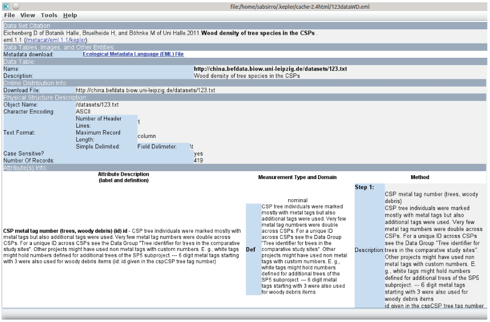
Figure 1. The EML 2 dataset component in use for the integration of the wood density dataset in the workflow.
On the right side the opened metadata window which displays all the additional information available for the dataset.
As the underlying analysis of the workflow continues in the projects we only provide a short insight in the still preliminary findings here. The carbon pool in the observational plots ranged from 5321.18 kg to 51,095.95 kg. The linear model revealed both species richness as well as stand age increased the carbon pool. In addition, there was a significant interaction between stand age and species richness in that the increase of carbon with stand age was less steep in plots with higher species richness (p-values for stand age: 0.0006, species richness: 0.0568 and their interaction: 0.0236).
Workflow design
We use the Kepler workflow system (version 2.4) to build our workflow. The components in Kepler fall into two categories: “actors”, which handle all kinds of data related tasks, and “directors”, which direct the execution of components in the workflow. The components in Kepler can “talk” to each other via a port system. Output ports of components hand over their data to input ports of another component2.
The “SDF” director was used to execute our workflow as it handles sequential workflows. The data was imported into Kepler using the “eml2dataset” actor. This actor can import datasets along the conventions of the Ecological Metadata Language16. The component reads the information available in the metadata file and uses it to automatically set up output ports to allow a direct consumption of the related data by other components in the workflow. The data in the underlying carbon stock analysis is manipulated mainly by using the rich statistics environment R17. From within Kepler we use the “RExpression” actor that offers an interface to R. We aimed at a uniform and low complexity for each workflow component. As a rule of thumb we set a limit of 5 lines of code per component.
Quantifying workflow complexity
To quantify the component complexity we used the number of code lines (loc), the number of R commands (cc) and R packages (pc) used, as well as the number of input and output ports (cp) of the component (equation 1). We further calculated a relative component complexity as the ratio of absolute complexity to total workflow complexity given by the sum of all component complexities (equation 2).
As each component in the workflow starts its operation only if all input port variables have arrived, the longest port connection of a component back to a data source defines its absolute position in the workflow sequence (Figure 2). We could thus explore total workflow complexity, individual component complexities, the number of components, and the number of identical tasks (see below) along the sequence of the workflow. For this we used linear models and compared them using Akaike Information Criteria (AIC)18.

Figure 2. This figure shows assigned component positions using the example of the herb layer dataset of the workflow.
The absolute position in a workflow is defined by the distance back to the data source. The numbers on the components display the distance count back to the data source. The assignment of positions starts with 0.
Quantifying component identity
Based on our analysis, we classified workflow components into 12 tasks a priori (Table 1). We then used text mining tools to characterize the components automatically. For this we used the presence/absence of R commands and libraries as qualitative values, the number of input and output ports, the number of datasets a component is connected with, as well as the count of code lines. This allowed us to match the a priori tasks with the automatically gathered characteristics. We used non metric multidimensional scaling (NMDS)19 to find the two main axes of variation in the multidimensional space defined by the characteristics. We then performed linear regression to identify which of the characteristics and which of the a-priori tasks could explain variation of the two NMDS axes. We could further compare task complexities. For this we used a Kruskal-Wallis test and a post-hoc Wilcoxon test, since residuals where not normally distributed (Shapiro-Wilk test).
Table 1. Workflow component tasks defined a priori in the analysis of a biodiversity effect on forest carbon pools and their relation to the data oriented motifs identified by
10
.
| Identities | Description | Motif |
|---|
| data source | Access (remote or local data) | Data retrieval |
| type transformation | Transform the type of a variable (e.g to numeric) | Data preparation |
| merge data | Match and merge data | Data organization |
| data aggregation | Aggregate of data | Data organization |
| create new vector | Create a vector filled with new data | Data curat./clean |
| data imputation | Impute data (e.g linear regressions on data
subsets) | Data curat./clean |
| modify a vector | Modify a complete vector by a factor or basic
arithmetic operation | Data organization |
| create new factor | Create a new factor | Data organization |
| data extraction | Extract data values (e.g from comment strings) | Data curat./clean |
| sort data | Sort data | Data organization |
| data modeling | All kinds of model comparison related operations
(ANOVA, AIC) | Data analysis |
Quantifying quality and usage of data sources
Data for the workflow comes from several data sources, differing in the number of columns as well as the number of processing steps needed within the workflow. We here introduce two measures of data column usage, one relative to the data source and one relative to the number of workflow components processing the data. We further introduce a quality measure of a data column by identifying a critical component within the workflow that signifies the actual analyses that answers our scientific question. We thus have workflow components that prepare data for the analysis and we have (few) workflow components that consume data for the analyses (Figure 3).
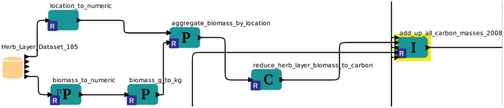
Figure 3. The usage and quality measure on an example dataset.
The components marked with a P represent preparation steps of a variable. Here we see three preparation steps so the quality is 4. The components marked with C and I represent direct consumption and an indirect influence. Those together build the variable usage together with all following influenced components.
As explained above, output ports of a data source in the workflow directly relate to data columns in the data set. Thus, the number of available ports of a data source is the “width” of a dataset, or the number of data columns. Thus, the usage of a data column in relation to the data source was calculated as the ratio of ports actually used in the workflow to the ports that were not used. This allowed us to relate the number of unused ports to the number of available ports of a data source.
In contrast, the usage of a data column in relation to the workflow is quantified by the total number of workflow components processing the data, before and after the actual analysis (equation 3). Similarly, the quality of a data column in relation to the workflow is quantified by the number of workflow components before the critical analysis, including this workflow component itself (equation 4). Thus, the higher the quality value, the lower the column’s quality. We can now compare datasets based to the usage and quality of their data as it is processed in the workflow. We did this using Kruskal-Wallis and post-hoc Wilcoxon tests.
The beginning matters - results from our workflow meta analysis
The workflow analysing carbon pools on a gradient of biodiversity consisted of 71 components in 16 workflow positions consuming the data of 8 datasets (Table 2). The data in the workflow was manipulated via 234 lines of R code. The number of code lines per component ranged between 1 (e.g component plot_2_numeric) and 23 (component impute_missing_tree_heights) with an overall mean of 3.3 (± 3.98 SD). See Figure 3 for a graphical representation of the workflow.
Table 2. The workflow positions listed along with the unique component tasks they contain and the count of components per position.
| Position | Tasks | Component
count |
|---|
| 0 | data source | 8 |
| 1 | data type transformation, data
extraction, create new vector | 20 |
| 2 | merge data, data imputation, modify
a vector, create new vector, data
aggregation, sort data | 10 |
| 3 | create new factor, merge data, data
aggregation | 7 |
| 4 | merge data, create new vector, data
imputation, modify a vector | 7 |
| 5 | create new vector, merge data, modify
a vector | 5 |
| 6 | merge data, data imputation, modify a
vector | 3 |
| 7 | data imputation, create new vector,
data aggregation | 3 |
| 8 | create new vector | 2 |
| 9 | merge data | 1 |
| 10 | modify a vector | 1 |
| 11 | data aggregation | 1 |
| 12 | modify a vector | 1 |
| 13 | create new vector | 1 |
| 14 | data modeling | 1 |
Although we aimed to keep the components streamlined and simple, the absolute and relative component complexity varied markedly. The absolute complexity ranged between 4 and 41 with an overall mean of 9.25 (± 6.77 SD), (Summary: Min. 4.0, 1st Qu. 4.0, Median 8.0, Mean 9.2, 3rd Qu. 12.0, Max. 41.0). Relative component complexity ranged between 0.69% (e.g component calculate_carbon_mass_from_biomass) and 7.03% (e.g component: add_missing_height _-broken_trees) with an overall mean of 1.59 (± 1.16 SD), (Summary: Min. 0.69, 1st Qu. 0.69, Median 1.37, Mean 1.59, 3rd Qu. 2.05, Max. 7.03).
Total workflow complexity decreased exponentially from the beginning to the end (Figure 4). The exponential decrease means that the decrease in complexity is steeper in the beginning of the workflow than at the end of the workflow, showing that complexity at the end of the workflow did not differ as much as at the beginning of the workflow. From the three models relating the sum of relative component complexities to workflow position, the one including position as logarithm (AIC = 64.69) was preferred over the one including a linear and a quadratic term for position (AIC = 65.67, delta AIC = 0.71), and the one including position as linear term only (AIC = 72.26, delta AIC = 7.3).
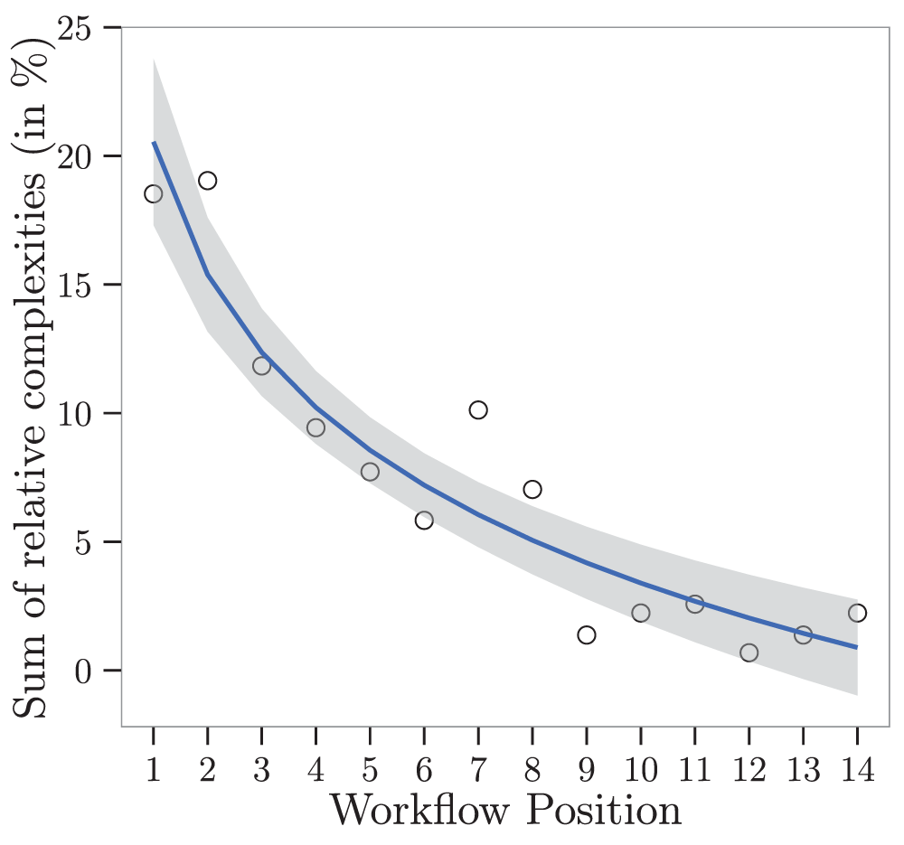
Figure 4. Relative workflow complexity along workflow positions could be best described by an exponential model including position as logarithm (R-squared=0.9, F-statistic: 29.16 on 3 and 10 DF, p-value: smaller than 0.001 ***).
This figure shows the model back transformed to the original workflow positions. The gray shading displays the standard error.
At the same time, relative complexity increased in the course of the analysis (Figure 5), since our model with an intercept and linear term for workflow position (AIC = 325.85) was preferred. However, we will argue later, that this increase was mainly due to a group of workflow components of extreme simplicity at the very beginning of data import, visible in the bottom left of Figure 5. These workflow components convert text columns into numeric columns in the “data type transformation” task. As we will outline later, we took this as an opportunity to program a feature for our data portal, to convert columns mixed with text and numbers to numeric columns for the EML output.
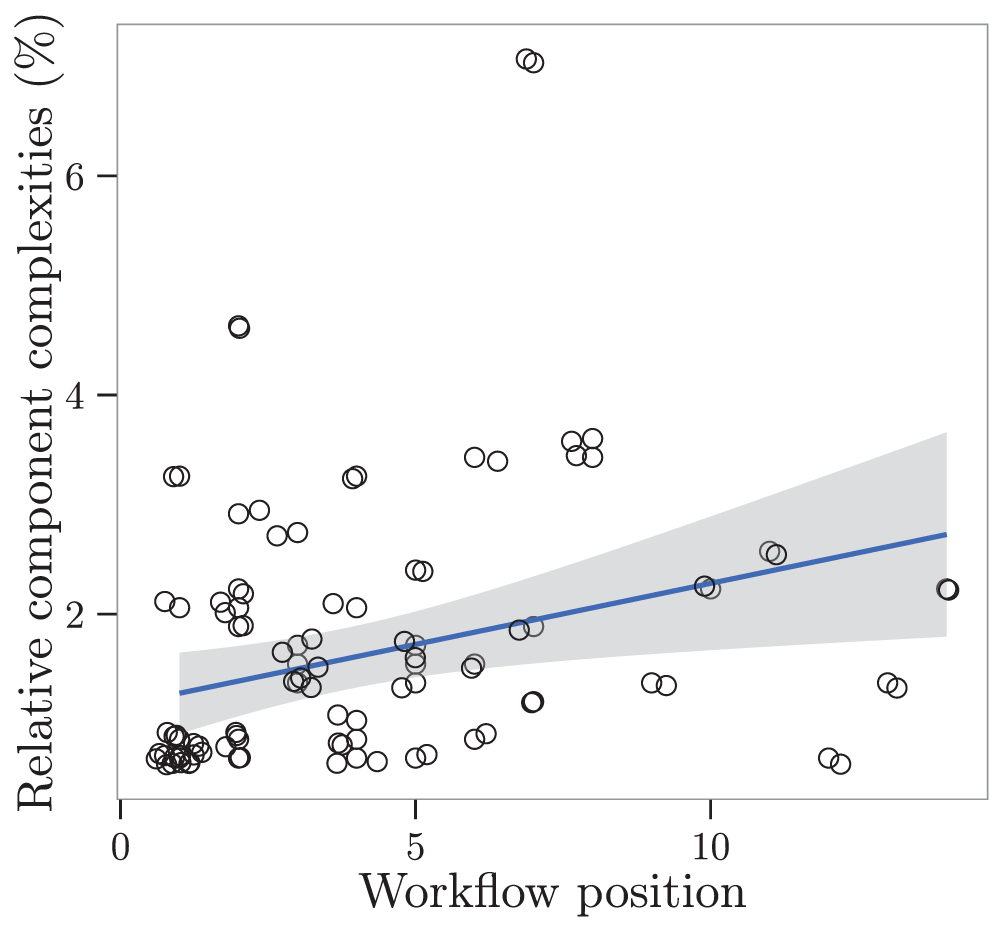
Figure 5. Relative component complexities along the workflow of the carbon analysis.
The points are slightly jittered to handle over plotting. At each position in the workflow there are components of different type and complexity. Linear model with positions as predictor for relative components complexity. R-squared: 0.09, F-statistic: 6.57 on 1 and 61 DF, p-value: 0.01285.
We could group workflow components according to their a priori assigned tasks using text mining. The non metric multidimensional scaling had a stress value of 0.17 using 2 main axes of variation. Several of the parameters, including specific commands of R code, were correlated to axes scores (Table 3). Our a priori defined tasks could be significantly separated in the parameter space (r2 0.58, p-value 0.001): the first axis spans between the workflow tasks “data aggregation” and “modify a vector” while the second one spans between the tasks “data extraction” and “data type transformation” (Figure 6).
Table 3. Results of the non metric multidimensional scaling of the component characteristics.
Signif. codes: 0 ‘***’ 0.001 ‘**’ 0.01 ‘*’ 0.05 ‘.’ 0.1 ‘ ’ 1. P-values based on 999 permutations.
| Characteristics | NMDS1 | NMDS2 | r2 | Pr(>r) | sig. |
|---|
| abline | -0.595118 | 0.803639 | 0.0879 | 0.024 | * |
| as.numeric | 0.229379 | -0.973337 | 0.3536 | 0.001 | *** |
| attach | -0.485526 | 0.874222 | 0.0535 | 0.113 | |
| data.frame | -0.902072 | -0.431586 | 0.8074 | 0.001 | *** |
| ddply | -0.802096 | -0.597195 | 0.3456 | 0.001 | *** |
| detach | -0.485526 | 0.874222 | 0.0535 | 0.113 | |
| grep | -0.211367 | 0.977407 | 0.2885 | 0.001 | *** |
| ifelse | -0.663695 | 0.748004 | 0.3222 | 0.001 | *** |
| is.na | -0.759568 | 0.650428 | 0.2800 | 0.001 | *** |
| length | -0.601172 | 0.799120 | 0.0526 | 0.182 | |
| lm | -0.199313 | 0.979936 | 0.0578 | 0.157 | |
| match | 0.445922 | 0.895072 | 0.0057 | 0.849 | |
| mean | -0.994320 | 0.106435 | 0.1346 | 0.016 | * |
| none | 0.977510 | 0.210891 | 0.5095 | 0.001 | *** |
| plot | -0.689676 | 0.724118 | 0.0478 | 0.254 | |
| predict | -0.595118 | 0.803639 | 0.0879 | 0.024 | * |
| sort | -0.417914 | -0.908487 | 0.0071 | 0.954 | |
| strsplit | 0.016877 | 0.999858 | 0.0633 | 0.059 | . |
| subset | -0.788938 | -0.614472 | 0.0212 | 0.821 | |
| sum | -0.658793 | -0.752324 | 0.1278 | 0.004 | ** |
| summary | 0.022488 | -0.999747 | 0.0043 | 0.969 | |
| unique | -0.485526 | 0.874222 | 0.0535 | 0.113 | |
| unlist | 0.016877 | 0.999858 | 0.0633 | 0.059 | . |
| vector | -0.269756 | 0.962929 | 0.4583 | 0.001 | *** |
| which | -0.421341 | 0.906902 | 0.4582 | 0.001 | *** |
| write.csv | 0.022488 | -0.999747 | 0.0043 | 0.969 | |
count of R
functions | -0.796351 | 0.604834 | 0.4893 | 0.001 | *** |
count of
codelines | -0.530470 | 0.847704 | 0.5392 | 0.001 | *** |
| domain count | 0.920778 | -0.390087 | 0.0142 | 0.704 | |
count packages
per component | -0.781994 | -0.623286 | 0.4004 | 0.001 | *** |
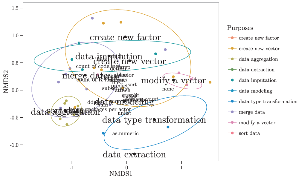
Figure 6. Non metric multi-dimensional scaling using the qualitative and quantitative component characteristics.
The scaling was created using the R package vegan with the Bray-Curtis distance. The large labels represent the workflow tasks. The smaller text annotations represent the characteristics used. They are slightly jittered by a factor of 0.2 horizontally and vertically to handle over plotting.
Our workflow tasks had similar complexity, with only one exception: the task “data type transformation” was less complex (Kruskal-Wallis chi-squared = 41.97, df = 9, p < 0.001) than the tasks create new vector, data aggregation, data imputation and merge data (Figure 7). Again, data type transformation was only used at the beginning of the workflow to transform columns mixing numbers and text to numbers.
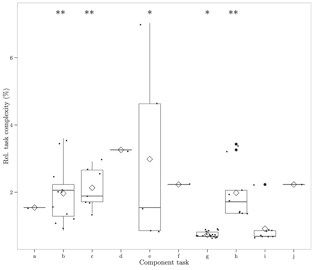
Figure 7. The median, 25% and 75% quantiles of the relative component complexities for the component tasks.
Letters refer to: a=create new factor, b=create new vector, c=data aggregation, d=data extraction, e=data imputation, f=data modeling, g=data type transformation, h=merge data, i=modify a vector, j=sort data. The small dots are the relative complexities, the diamonds the means. The whiskers are 25% quantile - 1.5 * IQR and 75% quantile + 1.5 * IQR, big black circles are outliers. Signific.: * = 0.05, ** = 0.001.
Data usage in relation to data sources was higher in smaller data sources. “Wide” data sources, those consisting of many columns, contributed less to the analysis than “smaller” data sources with fewer columns. While on average 37.4% of the columns in the data sources were used, a linear regression showed that the number of columns not used increased with the total number of columns available per data source (Figure 8).
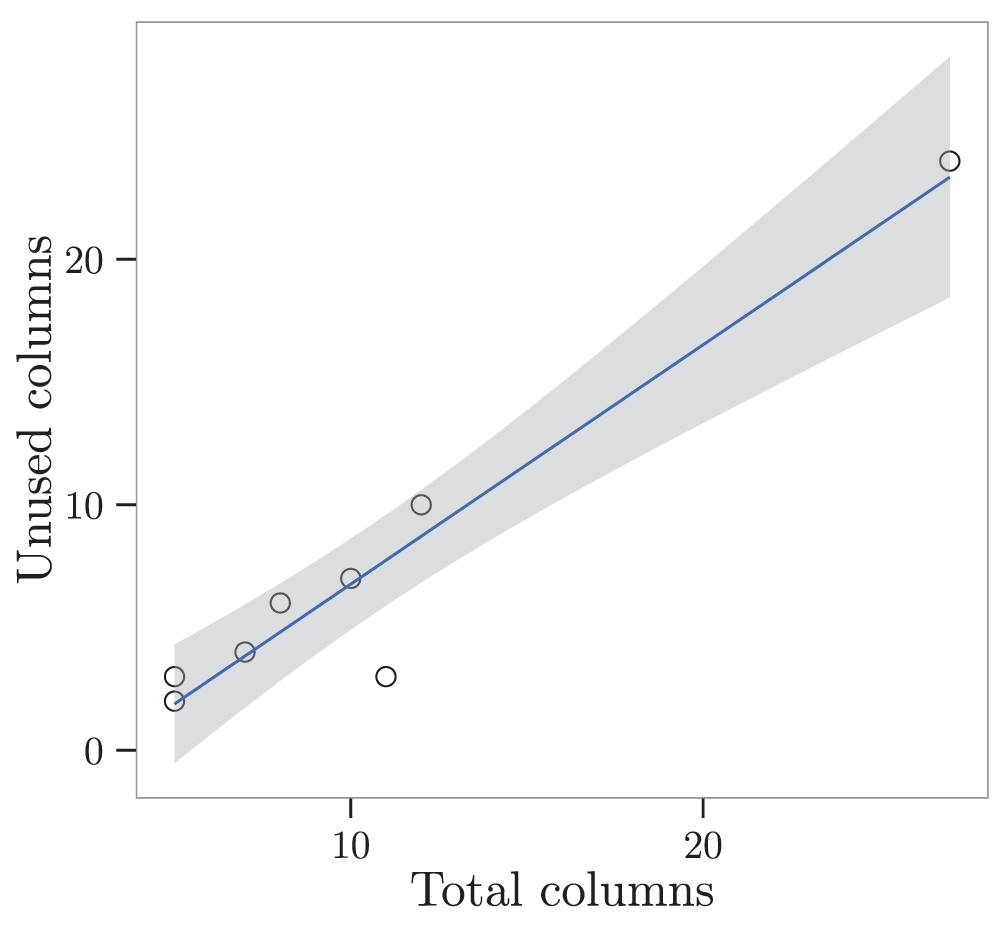
Figure 8. The linear regression shows the dependency between the total column count of the datasets and the count of unused columns.
The gray shaded area represents the standard error. Linear model with total columns as predictor for unused columns: R-squared: 0.925, F-statistic: 74.02 on 1 and 6 DF, p-value: 0.0001.
At the same time, data usage in relation to the workflow was similar for all data sources. Data column usage within the workflow ranged between a minimum of 1 and a maximum of 16 with an overall mean of 6.38 (± 4.25 SD). Although usage was different between datasets (Kruskal-Wallis, chi-squared = 18.05, df = 7, p-value = 0.012), a post hoc group wise comparison could not identify the differences (Wilcoxon test). The data column quality, the amount of processing steps needed to transform data for the analysis (see above), was also similar for all data sources. It ranged between a minimum of 1 and a maximum of 10 with an overall mean of 3.54 (± 2.44 SD). There were no differences in the data column quality between data sources (Kruskal-Wallis, chi-squared = 10.9, df = 7, p-value = 0.14).
Discussion
We showed that workflow complexity and data usage of a typical analysis in BEF can be quantified using relatively simple qualitative and quantitative measures based on commands, code lines, and variable numbers. It is the data aggregation, merging, and subsetting part at the beginning that complicates workflows. In our case, workflow complexity decreased exponentially in the course of the analysis (Figure 4). Similarly,10 found that the data transformation, merging and aggregation steps at the beginning of an analysis complicate workflows. Thus, simplifying data processing steps would greatly increase workflow simplicity. Here we argue that data simplicity could be fostered by providing feedback to data providers on the usage and quality values of the columns in their datasets14.
In our workflow, “wide” datasets consisting of many columns, contributed less to the analysis than smaller datasets with fewer columns (Figure 8). The more data columns a dataset has, the more difficult it is to understand what the dataset is about. The more data columns it has, the more difficult it is to describe it. The high number of columns in datasets resulting from fieldwork in ecology is a result of the effort to provide comprehensive information in one file only, often including different experimental designs and methodologies. These datasets result from copying field notes that are related to the same research objects, but combine information from different experiments. For example, a field campaign on estimating the amount of woody debris on a study site might count the number and size of branches found. At the same time, as one is already in the field, other branches might be used to find general rules for branch allometries. Thus, the same sheet of paper will be used for two different purposes. While this approach is efficient in terms of time and field work effort, it leads to highly complicated datasets. Separating the datasets into two, one for the dead matter, the other for branch allometries would decrease the number of columns of a dataset and increase the value of the dataset for the analysis of carbon budgets.
Combining data from different sources for meta-analyses could especially benefit from a more atomic way of storing data. Atomic means data particles (e.g. columns) stored separately, described via metadata and linked to ontological concepts. But in ecology the linking of data is rarely performed due to the high heterogeneity of data and concepts. With emerging technologies and a broader acceptance of metadata and ontological frameworks in ecology, datasets could be created automatically using logical constraints built from available atomic data particles. So, a query could return horizontal and vertically subsetted data products (facets) that, in the best case scenario, represent a 100% match directly usable in a meta-analysis20.
Providing feedback to data providers about the complexity of their data may thus be an important step in leveraging the readability of scientific workflows and supporting the reproducibility of data-driven science. This is especially true for “dark” data, the small and complex datasets in the long tail of big data4. We are presently witnessing a growing concern over the loss of data21, which is mostly due to the illegibility of datasets due to missing metadata and the lack of adherence to standard formats. Researchers still do not have training in data management. This concern in losing complex data has led to the invention of tools like DataUP that help to annotate data within Excel, or BEFdata to import Excel files, since this spreadsheet software is mainly used for data storage by researchers. At the same time, opportunities are emerging to publish datasets (Ecological Archives is only one alternative, there are also data journals http://www.hindawi.com/dpis/ecology/) and to provide measures of impact for data22.
Providing means for data quality feedback may also be helpful for propagating data ownership, which remains an unsolved problem14 and a major concern in data sharing23,24. We show that in our analysis, all data columns had a similar usage factor in relation to the workflow. Such usage factors could help to quantify data ownership as they allow one to quantify the amount a certain column or dataset has contributed to derive the results of an analysis.
Since we used the Kepler workflow software to execute R scripts, we made use of Kepler’s interface components. Our text-based approach of quantifying complexity will thus be useful mainly in the context of workflows that work with custom scripts. However, the Kepler workflows are stored as XML files and our approach could thus be generalized to other components in Kepler, or other workflow systems working with XML as an exchange format. Even if workflow programs do not store their workflows in human readable form, their source code could be analysed using similar text-based measures. Providing complexity measures at the level of workflow components might help in re-using and adapting workflows.
To date, the workflow platform “MyExperiment” is used by 7500 members and presents 2500 workflows for reuse and adaption, however, there is only a rating for the workflow. Offering complexity measures for workflow components may help to identify bottlenecks in existing workflows and help users to adapt components of workflows25, http://www.myexperiment.org/workflows?query=ecology).
A further step in finding and adapting workflows would be the possibility to identify useful workflow components. Here we show that we could identify workflow tasks using text mining (Figure 6). In our case, we could identify one task of very low complexity (data type transformation). This task was very simple and constituted the second axis of our NMDS (Figure 6). Components of this task mostly convert text vectors into numeric vectors. Having text vectors that could actually be interpreted as numbers stems from a “weakness” of EML, in that it does not allow text in data columns that store numbers. However, it is very common that scientists comment missing values or numbers below or above a measuring uncertainty threshold using text. To store the datasets in EML format forces the data provider to label the whole column as a text column.
As a consequence of having identified this simple and repetitive task of converting text to numbers, we have now added a feature to the BEFdata platform application that automates the conversion. We now offer two ways of exporting the data as comma separated values (CSV), one using the original data and one duplicating numeric columns that contain text, one column containing only the numbers, the other containing only the text. This is also the procedure suggested by DataUP for dealing with columns mixing text and numbers26. The BEFdata EML export now only offers the data in the latter format, so that numbers are no longer mixed with text. This is an example of how the analysis of a scientific workflow can guide towards useful automation features for data repositories.
Summary
Simplicity of data sources is the key to simple workflows, but we currently lack feedback mechanisms for quantifying data simplicity. We show that simple text-based measures could already be helpful in quantifying data and workflow complexity. Providing feedback on data complexity as well as the complexity of workflow components may not only foster simplicity and reuse, but additionally may present a means of propagating data ownership through interdisciplinary synthesis efforts and highlights the importance of the underlying primary research data.
Data availability
figshare: Data used to quantify the complexity of the workflow on biodiversity-ecosystem functioning, http://dx.doi.org/10.6084/m9.figshare.100831927
Author contributions
C.T.P., K.N., S.R., C.W. and H.B. substantially contributed to the work including the conceptualization of the work, the acquisition and analysis of data as well as critical revision of the draft towards the final manuscript.
Competing interests
No competing interests were disclosed.
Grant information
The data was collected by 7 independent projects of the biodiversity - ecosystem functioning - China (BEF-China) research group funded by the German Research Foundation (DFG, FOR 891).
Acknowledgements
Thanks to all the data owners from the BEF-China experiment who contributed their data to make this analysis possible. The research data is not all publicly available currently but will be in future. The datasets are linked and the ones publicly available are marked accordingly and can be downloaded using the following links. By dataset these are: Wood density of tree species in the Comparative study plot (CSPs): David Eichenberg, Martin Böhnke, Helge Bruelheide. Tree size in the CSPs in 2008 and 2009: Bernhard Schmid, Martin Baruffol. Biomass of herb layer plants in the CSPs, separated into functional groups (public): Alexandra Erfmeier, Sabine Both. Gravimetric Water Content of the Mineral Soil in the CSPs: Stefan Trogisch, Michael Scherer-Lorenzen. Coarse woody debris (CWD): Collection of data on dead wood with special regard to snow break (public): Goddert von Oheimb, Karin Nadrowski, Christian Wirth. CSP information to be shared with all BEF-China scientists: Helge Bruelheide, Karin Nadrowski. CNS and pH analyses of soils depth, increments of 27 Comparative Study Plots: Peter Kühn, Thomas Scholten, Christian Geißler.
Faculty Opinions recommendedReferences
- 1.
Michener WK, Jones MB:
Ecoinformatics: supporting ecology as a data-intensive science.
Trends Ecol Evol.
2012; 27(2): 85–93. PubMed Abstract
| Publisher Full Text
- 2.
Altintas I, Berkley C, Jaeger E, et al.:
Kepler: an extensible system for design and execution of scientific workflows. Proceedings. 16th International Conference on Scientific and Statistical Database Management. 2004; 423–424. Publisher Full Text
- 3.
Ewa D, Gurmeet S, Mei-hui S, et al.:
Pegasus: a framework for mapping complex scientific workflows onto distributed systems. 2005; 13: 219–237. Reference Source
- 4.
Heidorn PB:
Shedding light on the dark data in the long tail of science.
Library Trends.
2008; 57(2): 280–299. Publisher Full Text
- 5.
Gries C, Porter JH:
Moving from custom scripts with extensive instructions to a workflow system: use of the Kepler workflow engine in environmental information management. In M B Jones and C Gries, editors, Environmental Information Management Conference 2011. Santa Barbara, CA University of California. 2011; 70–75. Reference Source
- 6.
Ewa D, Gurmeet S, Mei-hui S, et al.:
Pegasus: a framework for mapping complex scientific workflows onto distributed systems. 2005; 13: 219–237. Reference Source
- 7.
Oinn T, Greenwood M, Addis M, et al.:
Taverna: lessons in creating a workflow environment for the life sciences.
Concurrency Computation: Pract Exp.
2006; 18(10): 1067–1100. Publisher Full Text
- 8.
Bowers S, Ludäscher B:
Towards Automatic Generation of Semantic Types in Scientific Workflows. Web Information Systems Engineering–WISE 2005 Workshops Proceedings. 2005; 3807. : 207–216. Publisher Full Text
- 9.
McCabe TJ:
A complexity measure. In Proceedings of the 2nd international conference on Software engineering. ICSE ’76, Los Alamitos, CA USA. IEEE Computer Society Press. 1976; 2(4): 308–320. Publisher Full Text
- 10.
Garijo D, Alper P, Belhajjame K, et al.:
Common motifs in scientific workflows: An empirical analysis. IEEE 8th International Conference on E-Science. 2012; 1–8. Publisher Full Text
- 11.
Gil Y, González-Calero PA, Kim J, et al.:
A semantic framework for automatic generation of computational workflows using distributed data and component catalogues.
J Experimental Theoretical Artificial Intelligence.
2011; 23(4): 389–467. Publisher Full Text
- 12.
Nadrowski K, Ratcliffe S, Bönisch G, et al.:
Harmonizing, annotating and sharing data in biodiversityecosystem functioning research.
Methods Ecol Evol.
2013; 4(2): 201–205. Publisher Full Text
- 13.
Parsons MA, Godoy O, LeDrew E, et al.:
A conceptual framework for managing very diverse data for complex, interdisciplinary science.
J Info Sci.
2011; 37(6): 555–569. Publisher Full Text
- 14.
Ingwersen P, Chavan V:
Indicators for the Data Usage Index (DUI): an incentive for publishing primary biodiversity data through global information infrastructure.
BMC Bioinformatics.
2011; 12(Suppl 15): S3. PubMed Abstract
| Publisher Full Text
| Free Full Text
- 15.
Bruelheide H:
The role of tree and shrub diversity for production, erosion control, element cycling, and species conservation in Chinese subtropical forest ecosystems. 2010. Reference Source
- 16.
Fegraus EH, Andelman S, Jones MB, et al.:
Maximizing the value of ecological data with structured metadata: an introduction to ecological metadata language (eml) and principles for metadata creation.
Bulletin of the Ecological Society of America.
2005; 86(3): 158–168. Publisher Full Text
- 17.
R Development Core Team. R: A Language and Environment for Statistical Computing. R Foundation for Statistical Computing, Vienna, Austria, ISBN 3-90005107-0, 2008. Reference Source
- 18.
Burnham KP, Anderson DR:
Model selection and multimodel inference: a practical information-theoretic approach. Springer. 2002; 172. Reference Source
- 19.
Dixon P:
Vegan, a package of r functions for community ecology.
J Vegetation Sci.
2003; 14(6): 927–930. Publisher Full Text
- 20.
Leinfelder B, Bowers S, Jones MB, et al.:
Using Semantic Metadata for Discovery and Integration of Heterogeneous Ecological Data.
Language.
2011; 92–97.
- 21.
Nelson B:
Data sharing: Empty archives.
Nature.
2009; 461(7261): 160–163. PubMed Abstract
| Publisher Full Text
- 22.
Piwowar H:
Altmetrics: Value all research products.
Nature.
2013; 493(7431): 159–159. PubMed Abstract
| Publisher Full Text
- 23.
Cragin MH, Palmer CL, Carlson JR, et al.:
Data sharing, small science and institutional repositories.
Philos Trans A Math Phys Eng Sci.
2010; 368(1926): 4023–38. PubMed Abstract
| Publisher Full Text
- 24.
Xiaolei H, Hawkins BA, Fumin L, et al.:
Willing or unwilling to share primary biodiversity data: results and implications of an international survey.
Conservation Letters.
2012; 5(5): 399–406. Publisher Full Text
- 25.
De Roure D, Goble C, Bhagat J, et al.:
myexperiment: Defining the social virtual research environment. In eScience, 2008. eScience ’08. IEEE Fourth International Conference on. 2008; 182–189. Publisher Full Text
- 26.
DataUp. The dataup tool. developed by the california digital library and microsoft research connections with funding from gordon and betty moore foundation. 2013. Reference Source
- 27.
Pfaff CT, Nadrowski K, Ratcliffe S, et al.:
Data used to quantify the complexity of the workflow on biodiversity-ecosystem functioning.
Figshare.
2014. Data Source
Comments on this article Comments (0)