Revised
Amendments from Version 1
I would like to thank the reviewers for their comments. In response to the referees I made available a pre-compiled version of the executables for Windows and a corrected version of the R scripts tested under that operative system (available at https://github.com/lsaravia/mfsba/releases and doi: 10.5281/zenodo.8481). I added the description of the program to perform a randomization confidence envelope that is included in mfSBA. The following is a summary of the changes made to the manuscript:
• I have added some examples and clarifications to the introduction.
• I have explained that the SRS/MFA methodology is novel; I do not intend to make a comparison with other methods here, but present a description of the capabilities of the software. I also included an interpretation of multifractal spectra Dq based on Hill’s generalized diversity.
• The limitations of mfSBA have been more clearly stated.
• I have included an explanation on why Dq’s are different for Figure 2, which also helps the interpretation of SRS.
• I have included a supplementary figure comparing a multispecies spatial distribution generated by a neutral model.
To read any peer review reports and author responses for this article, follow the "read" links in the Open Peer Review table.
Introduction
Multifractals and fractals are related techniques mainly used in physics to characterize the scaling behavior of a system; they differ in that fractals look at the geometry of presence/absence patterns, while multifractals look at the arrangement of quantities such as population densities or biomass1. Scaling laws are an emergent general feature of ecological systems, and there is no a priori reason that power laws apply to ecological communities. If they do apply, they reflect constraints in their organization that can provide clues about the underlying mechanisms2,3. For example: in semi-arid vegetation patterns, power-laws are produced by facilitative interactions between plants against water scarcity4,5. In inter-tidal mudflat ecosystems the loss of power-law patterns is indicative of a degradation of the system6. Changes in power-law vegetation patterns can signal the transition from a facilitation-dominated regime to a competition-dominated one7. The previous examples deal with patch-size distributions but in several cases the definition of patches is not simple. Such cases are handled naturally by multifractals because they use densities or biomass directly.
Multifractals require that the object under study should be statistically self-similar, which means that a power-law could be fitted to data in a range of scales. But that does not mean that the power-law must be the best possible model. We can analyze the data without claiming that it is an exact multifractal8. One of the advantages of multifractals is that they require fewer conditions on data than more classical statistics such as autocorrelation and variograms. These usually require isotropy and stationarity9 but multifractals can be used with anisotropic data10 and are inherently non-stationary11,12. Anisotropy and non-stationarity are often seen in spatial ecological distributions13.
Multifractals are associated with systems governed by random multiplicative processes14. In ecological systems, these processes can be given as the interaction of survival probabilities and compound growth15. Moreover, the presence of multiplicative process is argued to produce the log-normal-like shape of species-abundance distributions16. Also, random processes with spatial correlations can generate multifractals14; these kind of processes are part of neutral community models17,18 and are observed in natural communities19. Thus there are a priori reasons to think that multifractals can be applied to spatial ecological data. Indeed, they have been applied to vegetal communities20, tropical forest21, microphytobentos and periphyton biomass patterns1,22, and to the characterization of species-area relationships23–25.
Rank-abundance distributions are a representation of species-abundance distributions (SAD) that are a classical description of communities26. These have been used to compare different communities and to compare models and data, but different mechanisms can produce nearly identical SADs27. SADs are often presented using rank-abundance diagrams (RAD) where the log-abundance is plotted on the y-axis vs. rank on the x-axis26. RADs are equivalent to cumulative distributions28 and thus are a robust way to visualize the SAD without losing information29. If the rank of each species is incorporated in its spatial distribution, it forms a surface: the species-rank surface (SRS). This SRS can be analyzed and compared using multifractals.
Here I present an open source software package that can be used for quantitative multifractal analysis (MFA) of densities, biomass or other continuous variables distributed in space. In addition the software can analyze SRS using MFA, though this kind of analysis is completely novel. A detailed description of the advantages of using SRS and MFA is outside the scope of this work and will be presented elsewhere. This software represents a step to make easier the use of multifractals for spatial pattern analysis in ecology. One of its advantages is that it can be integrated with another widely used software for quantitative analysis: the R statistical software30.
Multifractal analysis
Several good introductions to multifractal methods applied to ecology are available20,31; thus I will only give a brief overview. Multifractals analyze the scaling properties of quantities distributed in a space that we assume to be two dimensional (a plane), but MFA can be used with one dimensional (time series) or three dimensional data32. A classical way to characterize multifractals is using the generalized dimensions Dq33, also called Renyi dimensions34. Dq has been used to portray the probabilistic structure of attractors derived from dynamical systems10.
Another way to characterize multifractals is using the so called spectrum of singularities. This spectrum describes multifractals as interwoven sets each one with a singularity exponent α and a fractal dimension f(α)35. The two multifractal representations are equivalent, they display the same information in a different format. But with the spectrum of singularities, two quantities are estimated (α & f (α)) from data and are obtained with error. Instead, with generalized dimension only one quantity is estimated Dq, thus this method is preferred for statistical comparisons.
The multifractal spectra Dq, is related to the Hill’s generalized diversity index Nq, where q is an arbitrary real number36. There are special cases of q that are of common use in ecology: for q = 0 Nq corresponds to the number of species, q = 1 to the Shannon index, and q = 2 to the reciprocal of the Simpson’s diversity index. Thus Nq defines different diversity measures as q changes, which vary in their sensitivity to rare species. In a similar way Dq focuses on regions of the plane with higher densities if q is greater and in regions with lower densities if q is lower or negative.
There are two important differences, the first is that Nq is calculated at one predetermined scale of measurement, and Dq is related to how Nq changes with scale37. The second difference is that Dq can be calculated on any quantity distributed in space, not only the number of species. The multifractal formalism was originally developed for additive quantities38, and was later extended to non-additive quantities39. This means that to apply MFA, the quantity distributed over space must increase in a mathematical sense. For example, if you have ten species in an area A1 and ten species in an area A2 the number of species in the sum A1+A2 will be greater than or equal to ten. If the number of species were additive the sum A1+A2 has to be 20, but that is not generally true. A limitation of mfSBA in its present version is that it only estimates multifractal spectra for additive quantities.
Estimation
To estimate multifractal spectra I used the method of moments based on box-counting38. I estimate generalized dimensions and the spectrum of singularities at the same time using the canonical method35. Here I describe only the Dq estimation; the steps for α and f (α) estimation are identical (only the formulae to calculate the quantities are different and can be found in the appendix of Saravia et al. (2012)1).
The spatial distribution that we are analyzing is covered with a grid, which is divided into N (∈) squares of side ∈. The contents of each square is called μi(∈). Then the so called partition function is computed as:
Where q is called moment order. The operation is performed for different values of ∈ and q, within a predetermined range. The generalized dimension is calculated as:
When q = 1, the denominator of the first term in Dq is undefined, so it must be replaced by the following expression:
In practical cases, as the limit can not be assessed, the dimensions are estimated as the slope of log(Zq) versus log(∈) (Figure 1) divided by q – 1 as shown in equation (1). This is done for different q, provided that it is a real number which yields a graph of Dq in terms of q, called the spectrum of generalized dimensions (Figure 2).
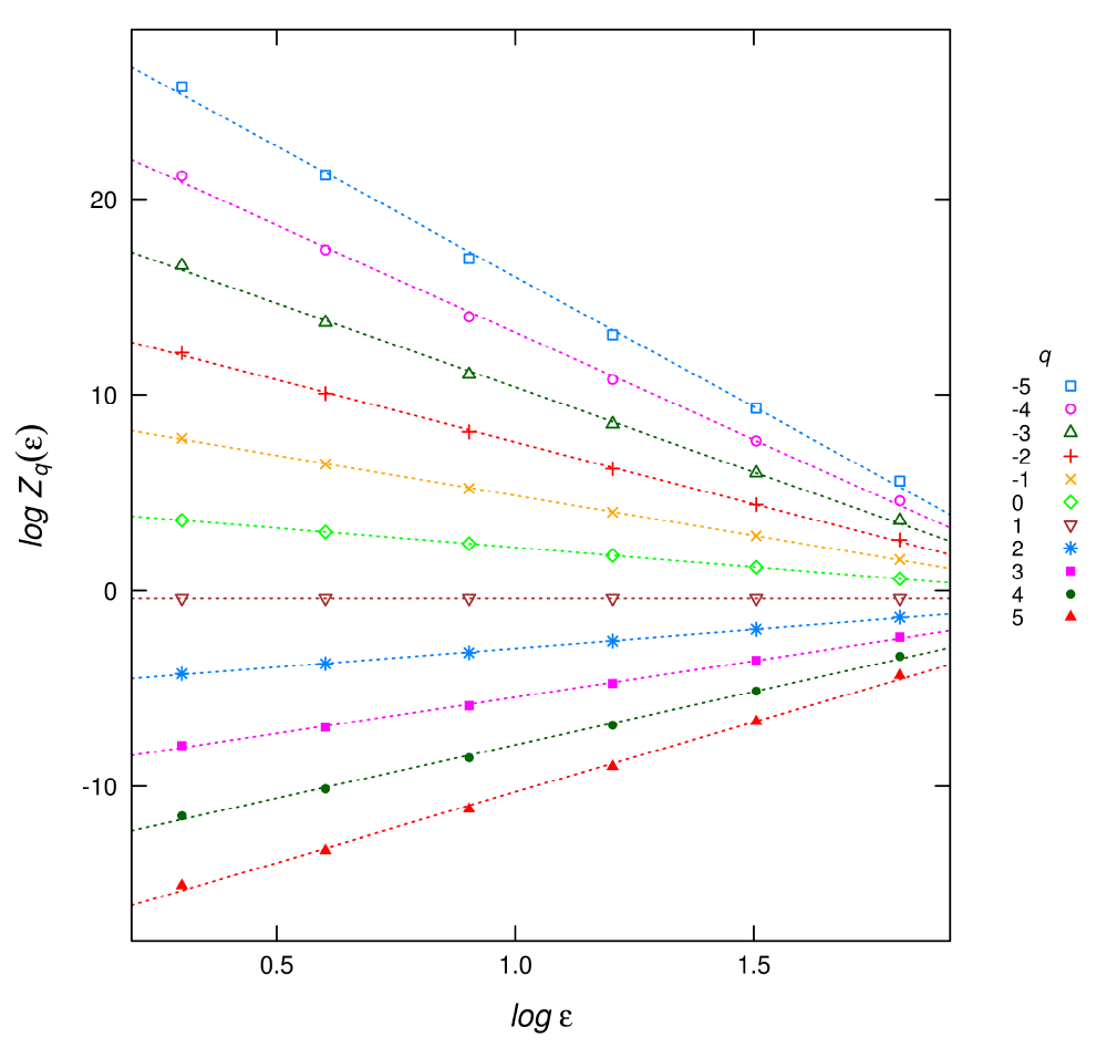
Figure 1. Plot of the linear regressions for different q used to estimate the Dq multifractal spectrum.
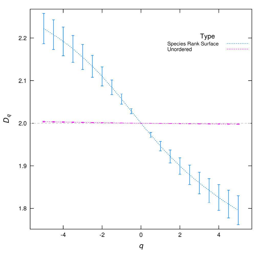
Figure 2.
Dq multifractal spectrum calculated from species spatial distributions.
If the multispecies distribution is analyzed unordered (with species numbers assigned by the simulation software) the Dq is almost flat corresponding to a uniform plus random noise distribution. But when the species rank surface (SRS) is used the Dq spectrum has a wide range of values, corresponding with a highly heterogeneous distribution, formed of valleys for the most abundant species and peaks for rare species. The error bars are the standard deviation obtained from the linear regressions used to estimate Dq.
To be an approximate multifractal, the relationship log(Zq) versus log(∈) should be well described by a linear relationship, although a linear relationship with superimposed oscillations is also acceptable31. A range of q and ∈ is fixed and then Dq is estimated using linear regressions. The coefficient of determination (R2) can be used as a descriptive measure of goodness of fit23.
Use of mfSBA software
The software was built and tested under Ubuntu 12.04 LTS Linux environment, using the GNU C++ compiler (v4.6.3). It requires the libtiff library for reading tiff images (http://www.libtiff.org/). It can be compiled under Windows environments using the GNU compiler and utilities for that operative system (http://www.mingw.org/).
You can download or clone mfSBA from https://github.com/lsaravia/mfsba (using git clone or as a zip file) and build it using the make utility.
make -f mfSBA.mak
You can run it from the command line using the following command structure:
mfSBA inputFile qFile minBox maxBox numBoxSizes option
the parameters are:
inputFile: this file can have only two formats: 1) one-layer tiff 2) “sed” file format. Sed is an ascii format I invented to use with my own stochastic cellular automata models to represent a square grid of values. It has a header of two lines: the first line describes the two dimensions X Y of the data, and the second line describes the type of data. For this program, the type must be BI, which means that the values stored in the grid are real numbers with double precision. See the example file with a “.sed” extension.
qFile: this is a sed file with a vector of values representing the q’s used to calculate the multifractal spectrum.
minBox,maxBox,numBoxSizes: Minimum box size, maximum box size and maximum number of box sizes. The program uses box sizes in powers of two: if maxBox is greater than half of the image size, it is set to that value. If the number of boxes between minBox and maxBox is greater than numBoxSizes, the latter number of boxes will be used, discarding the biggest ones.
option: is an upper case character with four possibilities: N,S,D,A.
– N: analyze the input file as is.
– S: normalize the input file then analyze it. Normalization is done summing all the pixels values and dividing each pixel by that total. After that the sum of all values is one.
– D: add 1 to all the pixels then normalize as in S.
– A: normalize as in S and save the normalized image as a sed file.
Examples of input files are included with the source code, thus after compiling you could run the following command assuming a linux system:
./mfSBA b4-991008bio.sed q21.sed 2 256 20 S
Output
The program generates four output files, attaching a prefix to the original input file name:
t.inputFile: this file has a header line with field names and q + 2 columns. The first two columns are the box sizes and log box sizes used in the estimation. After that, each column corresponds to log (Zq (∈)) of equation (2) with the q’s specified in the qFile. This file could be used to visually check the linearity assumptions to calculate Dq as in Figure 1.
a.inputFile & f.inputFile: are similar to the previous file, but used to calculate α and f (α). The formulae are described in the appendix of Saravia et al. (2012)1.
s.inputFile: this file has a header line with field names and 10 columns. The first column is q. The second column is called Tau and is the result of the regression to calculate the limit in equation 2. Thus to obtain Dq we have to divide it by q − 1, except in the case of q = 1 that we take the value of the next column to get Dq. The third column is the value of α and the forth column f (α). After that, columns are the corresponding coefficients of determination R2 and standard deviations.
Species rank surface
I propose to extend the analysis of SAD attaching the rank of each species to its spatial distribution. In this way, the multivariate spatial distribution of all species can be summarized into a univariate distribution. I called this spatial distribution the species-rank surface (SRS), and it can be analyzed and compared using MFA. To construct the SRS, I first calculate the rank-ordering of the species by their abundance from biggest to smallest, starting from one. Then the rank is assigned to the spatial position of the individuals of each species, forming a surface. This landscape has valleys formed by the most abundant species and peaks determined by the rarest species, and the standard MFA can be applied. SRS is additive, in the sense explained earlier, because ranks are not recalculated when the scale changes. The program used to calculate this is called multiSpeciesSBA, and is included with the mfSBA source code. You can compile it using the following command:
make -f multiSpeciesSBA.mak
Then all the input files and parameters are identical to mfSBA except that the program expects an inputFile containing a multispecies distribution. So the inputFile should be composed of integer numbers each one representing one species. An example of a sed file with a multispecies spatial distribution is given in t64-0100.sed, this file was obtained using a spatially explicit neutral model with 64 species (available at https://github.com/lsaravia/neutral). You can use the following command to perform the MFA:
./multiSpeciesSBA t64-0100.sed q21.sed 2 128 20 N
A confidence envelope for spatial randomness
To determine if Dq spectra are different from ones produced by a random spatial distribution of the quantity analyzed, I developed a randomization test. I shuffled all the positions of the original distribution and recalculated Dq. The procedure is repeated many times (e.g. 1000) and the highest and lowest tails determine a confidence envelope40. If the actual values of Dq falls outside the envelope the spatial pattern is not random for that particular q. This program can be compiled using the following command:
make -f mfSBArnz.mak
The command to run the analysis has a similar structure to the previous:
mfSBArnz inputFile outFile qFile minBox maxBox numBoxSizes option numSimul P
All the parameters previously mentioned have the same meaning, I will explain only the new ones:
outFile: this is the name of a file with all the Dq calculations specified with the numSimul parameter. It has the same format as the s.inputFile with an additional first column labeling the original Dq or a randomization. This file could be used to calculate the confidence envelope with a different P without doing the randomizations again. The program generates another file with an added “.rnz” extension, which contains the summarized results: the first row contains the number of randomizations and the size of the tail, the second row the p-value requested, the third row the field names, and from the fourth row there are five columns: the original values of q and Dq, two colums representing the randomization envelope at the requested p-level (DqMax & DqMin) and a column with 1/-1 indicating if the original Dq falls outside the envelope or 0 if it was inside the envelope.
numSimul: the number of randomizations, a bigger number will give a more accurate confidence envelope at the requested p-level41.
P: a two tailed p-value for the confidence envelope, that is the chance than Dq falls outside the envelope if the spatial pattern is random (Type I error).
An example of this analysis can be performed with the following command:
./mfSBArnz t64-0100.sed t64-0100 q21.sed 2 256 20 S 1000 0.05
If the software is used under Windows the name of the executable program should be changed, deleting “./” and adding the “.exe” extension, for this last example it should be mfSBArnz.exe.
R integration
Included with the source is a set of functions as an example to integrate the mfSBA software with the R language (http://www.r-project.org/). You should have compiled or downloaded the executables in the same folder as the R scripts. Then you can load the functions inside R with:
source('Fun_MFA.r')
and then run the same given examples:
dq1<− calcDq_mfSBA("b4-991008bio.sed","q21.sed 2 256 20 S")
An interesting example is to compare the Dq from the example multispecies spatial distribution untransformed
dq1<− calcDq_mfSBA("t64-0100.sed","q21.sed 2 512 20 S",T)
dq1$Site <− "Untransformed"
with the Dq from SRS
dq<− calcDq_multiSBA("t64-0100.sed","q21.sed 2 512 20 S",T)
dq$Site <− "Species Rank Surface"
dq <− rbind(dq,dq1)
and plot Dq with
plot_DqCI(dq)
In this plot (Figure 2), we can see that the two Dq spectra are different. The Dq calculated from the unordered distribution is nearly flat, this corresponds to an almost constant spatial distribution with uncorrelated random noise. The structure of SRS is lost when species are assigned with a different order, valleys are formed by the most abundant species and peaks of rare species are destroyed. This is similar to comparing a RAD with a figure made with the ranks disordered on the x axis. Although the species distribution is the same, the two surfaces are different (Supplementary Figure 1), which is reflected in their Dq spectra.
The plot of the t.inputFile (Figure 1) gives a visual check of the regressions to obtain Dq:
plotDqFit("t.t64-0100.sed","q21.sed")
additionally the R2 values could be easily checked:
hist(dq1$R.Dq)
All the examples and more graphics are included in the file testMFA.r, you should change this file to reflect the folder where you downloaded the software.
Conclusion
The multifractal spectrum can be used to describe and compare spatial patterns of biomass, density, height, point patterns, or any continuous variable. The condition is that the distribution of the variable in space must be additive. The mfSBA software is especially useful for remote sensing data because it can be used with tiff images. Multifractal patterns could be produced by the existence of multiplicative interaction between species and by spatially correlated random processes such as dispersal and growth14. Plant and animal species are generally aggregated in space thus is very likely that multifractal analysis can be used in a wide range of cases.
The analysis of SRS using Dq adds a new dimension to the comparison of species spatial distributions, because it can be used to compare spatial distributions of all species at the same time and also the abundances are accounted. An exploration of the results of different spatial patterns should be needed as a continuation of the present work.
The analysis of SRS using Dq adds a new dimension to the comparison of species spatial distributions, because it can be used to compare spatial distributions of all species at the same time and as the species ranks are used, this is a spatial version of SAD. The method presented here analyzes SRS as a surface, which is different to SAR and to multifractals calculated with the number of species as in Borda-de-Agua (2002)23. An exploration of SRS analysis resulting from different spatial patterns combined with different SADs will be needed as a continuation of the present work. Also the software should be extended to calculate MFA for non-additive distributions such as the number of species.
The software presented here is oriented to obtain multifractal spectra for comparisons, rather than to obtain the true value. While the estimation methods used in mfSBA could be improved31,42, it has been used without trouble with the kind of data obtained in ecological studies1,43.
Multifractals can be successfully used to analyze several aspects of community spatial structure. With the advent of the big data era in ecology44 and the use of new technology to acquire spatial data45
, new methods to analyze complex data sets are needed and multifractals could be an interesting addition to the ecologist’s toolbox.
Software availability
Zenodo: Multifractal estimation using a standard box-counting algorithm: version 2, doi: 10.5281/zenodo.848146
GitHub: Multifractal estimation using a standard box counting algorithm, https://github.com/lsaravia/mfsba
Competing interests
No competing interests were disclosed.
Grant information
The author(s) declared that no grants were involved in supporting this work.
Acknowledgments
I am grateful to Fernando R. Momo for our great conversations about ecological theory and David J. Harris for his language revision.
Supplementary material
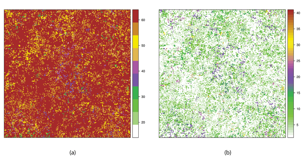
Supplementary Figure 1. Comparison of a multiespecies spatial distribution generated by a neutral model with 64 possible species.
Both figures represent the same species distribution but with diferent numeric values assigned to species. (a) The values are assigned by the simulation program. The most abundant species have higher values and the range 1–64 represents all posible species. (b) Spatial Rank Surface: each species is assigned to its rank as explained in the main text: the most abundant species has the lowest value and represent valleys, rare species represent peaks. The range is lower because some species did not appear.
Faculty Opinions recommendedReferences
- 1.
Saravia LA, Giorgi A, Momo F:
Multifractal growth in periphyton communities.
Oikos.
2012; 121(11): 1810–1820. Publisher Full Text
- 2.
Brown JH, Gupta VK, Li BL, et al.:
The fractal nature of nature: power laws, ecological complexity and biodiversity.
Philos Trans R Soc Lond B Biol Sci.
357(1421): 2002; 619–626. PubMed Abstract
| Publisher Full Text
| Free Full Text
- 3.
Solé RV, Bascompte J:
Self-organization in complex ecosystems. Princeton University Press, 2006. Reference Source
- 4.
Scanlon TM, Caylor KK, Levin SA, et al.:
Positive feedbacks promote power-law clustering of Kalahari vegetation.
Nature.
2007; 449(7159): 209–212. PubMed Abstract
| Publisher Full Text
- 5.
Kéfi S, Rietkerk M, Alados CL, et al.:
Spatial vegetation patterns and imminent desertification in Mediterranean arid ecosystems.
Nature.
2007; 449(7159): 213–217. PubMed Abstract
| Publisher Full Text
- 6.
Weerman EJ, Van Belzen J, Rietkerk M, et al.:
Changes in diatom patch-size distribution and degradation in a spatially self-organized intertidal mudflat ecosystem.
Ecology.
2012; 93(3): 608–618. PubMed Abstract
| Publisher Full Text
- 7.
Manor A, Shnerb NM:
Facilitation, competition, and vegetation patchiness: From scale free distribution to patterns.
J Theor Biol.
2008; 253(4): 838–842. PubMed Abstract
| Publisher Full Text
- 8.
Lévy Véhel J:
Introduction to the multifractal analysis of images. In: Fisher Y editor. Fractal Image Encoding and Analysis. Springer Verlag. 1998; 299–341.
- 9.
Fortin MJ, Dale MRT, ver Hoef J:
Spatial Analysis in Ecology.
Encyclopedia of Environmetrics.
John Wiley & Sons, Ltd. 2006. Publisher Full Text
- 10.
Harte D:
Multifractals: Theory and Applications. Chapman & Hall/CRC, 2001. Reference Source
- 11.
Laurie H, Perrier E:
A multifractal model for spatial variation in species richness.
Ecological Complexity.
2010; 7(1): 32–35. Publisher Full Text
- 12.
Bez N, Bertrand S:
The duality of fractals: roughness and self-similarity.
Theoretical Ecology.
2011; 4(3): 371–383. Publisher Full Text
- 13.
Plotkin JB, Chave J, Ashton PS:
Cluster analysis of spatial patterns in Malaysian tree species.
Am Nat.
2002; 160(5): 629–644. PubMed Abstract
| Publisher Full Text
- 14.
Stanley HE, Meakin P:
Multifractal phenomena in physics and chemistry.
Nature.
1988; 335: 405–409. Publisher Full Text
- 15.
McGill BJ:
Strong and weak tests of macroecological theory.
Oikos.
2003; 102(3): 679–685. Publisher Full Text
- 16.
May RM, Crawley MJ, Sugihara G:
Communities: patterns. In: May RM, McLean AR, editors. Theoretical ecology: principles and applications. New York: Oxford University Press. 2007; 111–131. Reference Source
- 17.
Houchmandzadeh B, Vallade M:
Clustering in neutral ecology.
Phys Rev E Stat Nonlin Soft Matter Phys.
2003; 68(6 Pt 1): 1–7. PubMed Abstract
| Publisher Full Text
- 18.
Yakimov BN, Iudin DI, Solntsev LA, et al.:
Multifractal analysis of neutral community spatial structure.
J Theor Biol.
2014; 343: 44–53. PubMed Abstract
| Publisher Full Text
- 19.
Condit R, Ashton PS, Baker P, et al.:
Spatial patterns in the distribution of tropical tree species.
Science.
2000; 288(5470): 1414–1418. PubMed Abstract
| Publisher Full Text
- 20.
Scheuring I, Riedi RH:
Application of multifractals to the analysis of vegetation pattern.
Journal of Vegetation Science.
1994; 5(4): 489–496. Publisher Full Text
- 21.
Manrubia SC, Solé RV:
Self-organized criticality in rainforest dynamics.
Chaos, Solitons & Fractals.
1996; 7(4): 523–541. Publisher Full Text
- 22.
Seuront L, Spilmont N:
Self-organized criticality in intertidal microphytobenthos patch patterns.
Physica A.
2002; 313(3–4): 513–539. Publisher Full Text
- 23.
Borda-de-Água L, Hubbell SP, McAllister M:
Species-Area Curves, Diversity Indices, and Species Abundance Distributions: A Multifractal Analysis.
Am Nat.
2002; 159(2): 138–155. PubMed Abstract
| Publisher Full Text
- 24.
Yakimov BN, Bossuyt B, Iudin DI, et al.:
Multifractal diversity-area relationship at small scales in dune slack plant communities.
Oikos.
2008; 117(1): 33–39. Publisher Full Text
- 25.
Laurie H, Perrier E:
Beyond species area curves: application of a scale-free measure for spatial variability of species richness.
Oikos.
2011; 120(7): 966–978. Publisher Full Text
- 26.
McGill BJ, Etienne RS, Gray JS, et al.:
Species abundance distributions: moving beyond single prediction theories to integration within an ecological framework.
Ecol Lett.
2007; 10(10): 995–1015. PubMed Abstract
| Publisher Full Text
- 27.
Chave J, Muller-Landau HC, Levin SA:
Comparing Classical Community Models: Theoretical Consequences for Patterns of Diversity.
Am Nat.
2002; 159(1): 1–23. PubMed Abstract
| Publisher Full Text
- 28.
Newman MEJ:
Power laws, Pareto distributions and Zipf’s law.
Contemporary Physics.
2005; 46(5): 323–351. Publisher Full Text
- 29.
Li L, Alderson D, Doyle JC, et al.:
Towards a Theory of Scale-Free Graphs: Definition, Properties, and Implications.
Internet Mathematics.
2005; 2(4): 431–523. Publisher Full Text
- 30.
R Core Team: R:
A Language and Environment for Statistical Computing. Vienna, Austria: R Foundation for Statistical Computing. 2013. Reference Source
- 31.
Borda-de-Água L, Hubbell SP, He F:
Scaling biodiversity under neutrality.
Scaling Biodiversity.
2007; 347–375. Reference Source
- 32.
Lopes R, Betrouni N:
Fractal and multifractal analysis: A review.
Med Image Anal.
2009; 13(4): 634–649. PubMed Abstract
| Publisher Full Text
- 33.
Grassberger P:
Generalized dimensions of strange attractors.
Phys Lett A.
1983; 97(6): 227–230. Publisher Full Text
- 34.
Renyi A:
Probability Theory. Amsterdam: North-Holland. 1970. Reference Source
- 35.
Chhabra AB, Jensen RV:
Direct determination of the f(alfa) singularity spectrum.
Phys Rev Lett.
1989; 62(12): 1327–1330. Publisher Full Text
- 36.
Hill MO:
Diversity and Evenness: A Unifying Notation and Its Consequences.
Ecology.
1973; 54(2): 427–432. Publisher Full Text
- 37.
Ricotta C:
From theoretical ecology to statistical physics and back: self-similar landscape metrics as a synthesis of ecological diversity and geometrical complexity.
Ecol Model.
2000; 125(2–3): 245–253. Publisher Full Text
- 38.
Halsey TC, Jensen MH, Kadanoff LP, et al.:
Fractal measures and their singularities: The characterization of strange sets.
Phys Rev A.
1986; 33(2): 1141–1151. PubMed Abstract
| Publisher Full Text
- 39.
Lévy Véhel J, Vojak R:
Multifractal Analysis of Choquet Capacities.
Adv Appl Math.
1998; 20(1): 1–43. Publisher Full Text
- 40.
Crowley PH:
Resampling methods for computation-intensive data analysis in ecology and evolution.
Ann Rev Ecol Syst.
1992; 23: 405–447. Publisher Full Text
- 41.
Wiegand T, Moloney KA:
Rings, circles, and null-models for point pattern analysis in ecology.
Oikos.
2004; 104(2): 209–229. Publisher Full Text
- 42.
De Bartolo SG, Primavera L, Gaudio R, et al.:
Fixed-mass multifractal analysis of river networks and braided channels.
Phys Rev E Stat Nonlin Soft Matter Phys.
2006; 74(2 pt 2): 26101. PubMed Abstract
| Publisher Full Text
- 43.
Saravia LA, Giorgi A, Momo F:
Multifractal spatial patterns and diversity in an ecological succession.
PLoS ONE.
2012; 7(3): e34096. PubMed Abstract
| Publisher Full Text
| Free Full Text
- 44.
Hampton SE, Strasser CA, Tewksbury JJ, et al.:
Big data and the future of ecology.
Front Ecol Environ.
2013; 11(3): 156–162. Publisher Full Text
- 45.
Michener WK, Jones MB:
Ecoinformatics: supporting ecology as a data-intensive science.
Trends Ecol Evol.
2012; 27(2): 85–93. PubMed Abstract
| Publisher Full Text
- 46.
Saravia LA:
Multifractal estimation using a standard box-counting algorithm.
ZENODO.
2014. Data Source


- I
... Continue reading I appreciate Dr. Yakimov's comments on the manuscript. As a response to them and to the reviewer's comments, I have made several changes in the version 2 of the article:About the neutral model, I used it as an example of a not random distribution of species, I added a more complete description in its github repository https://github.com/lsaravia/Neutral
References
1. Borda-de-Água L, Hubbell SP, He F, (2007). Scaling biodiversity under neutrality. Scaling biodiversity. Cambridge: Cambridge University Press. pp. 347–375.
About the neutral model, I used it as an example of a not random distribution of species, I added a more complete description in its github repository https://github.com/lsaravia/Neutral
References
1. Borda-de-Água L, Hubbell SP, He F, (2007). Scaling biodiversity under neutrality. Scaling biodiversity. Cambridge: Cambridge University Press. pp. 347–375.