Keywords
Feature selection, algorithms, R package, computational efficiency
Feature selection, algorithms, R package, computational efficiency
Given a target (response or dependent) variable Y of n measurements and a set X of p features (predictor or independent variables) the problem of feature (or variable) selection (FS) is to identify the minimal set of features with the highest predictability on the target variable (outcome) of interest. Why should researchers and practitioners perform FS? For a variety of reasons1: a) many features may be expensive (and/or unnecessary) to measure, especially in the clinical and medical domains; b) FS may result in more accurate models (of higher predictability) by removing noise while treating the curse-of-dimensionality; c) the produced parsimonious models are computationally cheaper and easier to understand and interpret; d) future experiments can benefit from prior feature selection tasks and provide more insight into the problem of interest, its characteristics and structure.
R contains thousands of packages, but only a small portion of them are dedicated to the task of FS, yet offering limited or narrow capabilities. For example, packages that accept few or specific types of target variables (e.g. binary and multi-class only). This leaves many types of target variables, for example percentages, left censored, positive valued, matched case-control data, etc., untreated. The availability of regression models for some types of data is rather small. Count data is such an example, for which Poisson regression is the only model considered in nearly all R packages. Most algorithms including statistical tests offer limited statistical tests, e.g. likelihood ratio test only. Almost all available FS algorithms are devised for large sample sized data, thus they cannot be used in many biological settings where the number of observations rarely (or never in some cases) exceeds 100, but the number of features is in the order of tens of thousands. Finally, some packages are designed for high volume data1 only.
In this paper we present MXM2; an R package that overcomes the above shortcomings. It contains many FS algorithms2, which can handle many and diverse types of target variables, while offering a pool of regression models to choose from and employ. There is a plethora of statistical tests (likelihood-ratio, Wald, permutation based) and information criteria (BIC and eBIC) to plug into the FS algorithms. Algorithms that work with small (and large) sample sized data, algorithms that have been customized for high volume data, and an algorithm that returns multiple sets of statistically equivalent features are some of the key characteristics of MXM.
Over the next sections, a brief qualitative comparison of MXM with other packages available on CRAN and Bioconductor is presented, its (dis)advantages are discussed, its FS algorithms and related functions are mentioned. Finally a demonstration takes place, applying some FS algorithms available in MXM on real high dimensional data.
When searching for FS packages on CRAN and Bioconductor repositories using the keywords "feature selection", "variable selection", "selection", "screening" and "LASSO", we detected 184 R packages until the 7th of May 20183. Table 1 shows the frequency of the target variable types those packages accept, while Figure 1 shows the frequency of R packages whose FS algorithms can treat at least one type of target variable, of those presented in Table 1. Table 2 presents the frequency of pairwise types of target variables offered in R packages and Table 3 contains information on packages allowing for less frequent regression models. Most packages offer FS algorithms that are oriented towards specific types of target variables, methodology and regression models, offering at most 3-4 options. Out of these 184 packages, 65 (35.32%) offer LASSO type FS algorithms, while 19 (10.32%) address the problem of FS from the Bayesian perspective. Only 2 (1.08%) R packages treat the case of FS with multiple datasets while only 4 (2.17%) packages are devised for high volume data.
The percentage-wise number appears inside the parentheses.
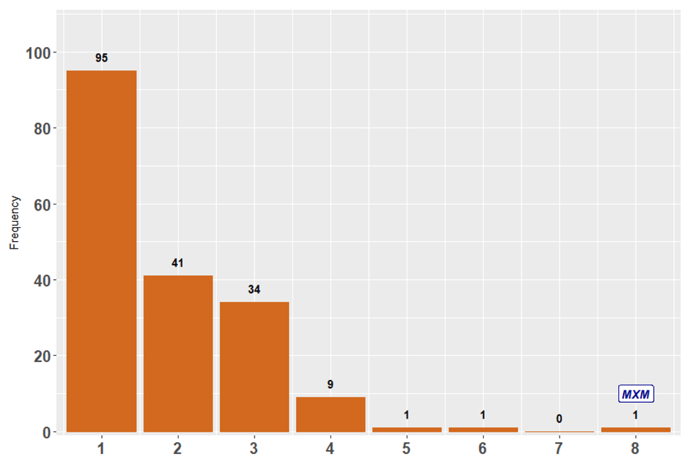
The horizontal axis shows the number of types (any combinations) of target variables from Table 1. For example, there 95 R packages that can handle only 1 type (any type) of target variable, 41 packages that can handle any 2 types of target variables, while MXM is the only one that handles all of them.
There are 108 packages which handle binary target variables, 59 packages offering algorithms for binary and continuous target variables and only one package handling ordinal and nominal target variables, etc.
The percentage-wise number appears inside the parentheses.
| Regression models | Robust | GLMM | GEE | Functional |
|---|---|---|---|---|
| Frequency (%) | 4 (2.19%) | 8 (4.37%) | 2 (1.09%) | 2 (1.09%) |
Table 4 summarizes the types of target variables treated by MXM’ FS algorithms along with the appropriate regression models that can be employed. The list is not exhaustive, as in some cases the type of the predictor variables (continuous or categorical) affects the decision of using a regression model or a test (Pearson and Spearman for continuous and G2 test of independence for categorical). With percentages for example, MXM offers numerous regression models to plug into its FS algorithms: beta regression, quasi binomial regression or any linear regression model (robust or not) after transforming the percentages using the logistic transformation. For repeated measurements (correlated data), there are two options offered, the GLMM and GEE methodologies which can also be used with various types of target variables, not mentioned here. We emphasize that MXM is the only package that covers all types of response variables mentioned on Table 1, many types of which are not available in any other FS package, such as left censored data for example. MXM also covers 3 out 4 cases that appear on Table 3.
Most of the currently available FS algorithms in the MXM package have been developed by the creators and authors of the package. These algorithms have been tested and compared with other state-of-the-art algorithms under different scenarios and types of data.
IAMB3 was on par with or outperforming competing machine learning algorithms, when both the target variable and features are categorical. MMPC and MMMB algorithms4 were tested in the context of BN learning showing great success with MMPC shown to achieve excellent false positive rates5. MMPC was also used as the basis of MMHC6, a prototypical algorithm for learning the structure of a Bayesian network which outperformed all other Bayesian network learning algorithms with categorical data. For time-to-event and nominal categorical target variable, MMPC 7, and 8 respectively, outperformed or was on par with LASSO and other FS algorithms. SES was contrasted against LASSO2 with continuous, binary and survival target variables, resulting in similar conclusions as before. With temporal and time-course data, SES9 outperformed the LASSO algorithm10 both in predictive performance and computational efficiency. FBED11 was compared with LASSO for the task of binary classification with sparse data exhibiting performance similar to that of LASSO. gOMP, a generalization of OMP12–14, has not been publicly tested, but our anecdotal experiments have showed very promising results, achieving similar or better performance, while enjoying higher computational efficiency than LASSO.
The main advantage of MXM is that all FS algorithms accept numerous and diverse types of target variables. MMPC, SES and FBED treat all types of target variables presented in Table 4, while gOMP handles fewer types4.
MXM is the only R package that offers many different regression models to be employed by the FS algorithms, even for the same type of response variable, such as Poisson, quasi Poisson, negative binomial and zero inflated Poisson regression for count data. For repeated measurements, the user has the option of using GLMM or the GEE methodology (the latter with more options in the correlation structure) and for time-to-event data, Cox, Weibull and exponential regression models are the available options.
A range of statistical tests and methodologies to select the features is offered. Instead of the usual log-likelihood ratio test, the user has the option to use the Wald test or produce a p-value based on permutations. The latter is useful and advised when the sample size is small, emphasizing the need for use of MMPC and SES, both of which are designed for small sample sized datasets. FBED on the other hand gives the option of using information criteria, BIC15 or eBIC16, instead of the log-likelihood ratio test.
Statistically Equivalent Signatures (SES)2,17 builds upon the ideas of MMPC and returns multiple (statistically equivalent) sets of predictor variables, making it one one of the few FS algorithms suggested in the literature, and available in hrefhttps://cran.r-project.org/CRAN, with this trait. 18 demonstrated that multiple, equivalent prognostic signatures for breast cancer can be extracted just by analyzing the same dataset with a different partition in training and test sets, showing the existence of several genes which are practically interchangeable in terms of predictive power. SES along with MMPC are two among the few algorithms, available on hrefhttps://cran.r-project.org/CRAN, that can be used with multiple datasets in a meta-analytic way, following 19.
MXM contains FS algorithms for small sample sized data (MMPC, MMMB, and SES) and for large sample sized data (FBED, gOMP). FBED and gOMP have been adopted for high volume data, going beyond the limits of R. The importance of these customizations can be appreciated by the fact that nowadays large scale datasets are more frequent than before. Since classical FS algorithms cannot handle such data, modifications must be made, in an algorithm level, in a memory efficient manner, in a computer architecture level, and/or in any other way. MXM is using an efficient memory handling R package.
Finally, many utility functions are available, such as constructing a model from the object an algorithm returned, construct a model in general, communication between the input and outputs of the algorithms, long verbose output with useful information, etc. Using hash objects, the computational cost of MMPC and SES is significantly reduced. The univariate associations computed from MMPC, SES and FBED can be interchanged among them and save computational time.
A disadvantage of most MXM’s algorithms is their computational efficiency. Their (algorithmic) order of complexity is comparable to state-of-art FS algorithms, but the nature of the other algorithms is such that many regression models must be fit increasing the computational burden. gOMP, for example, is the most efficient algorithm available in MXM5, because it is residual based and few regression models are fit. However, with clustered/longitudinal data, SES (and MMPC) were shown to scale to tens of thousands and be dramatically faster than LASSO9. Computational efficiency is also programming language-dependent. Most of the algorithms are currently written in R and we are constantly working towards transferring them to C++ so as to decrease the computational cost significantly.
It is impossible to cover all cases of target variables; we have no algorithms for time series, and do not treat multi-state time-to-event target variables for example, yet we search for R packages that treat other types of target variables and link them to MXM. All algorithms are limited to linear or generalized linear relationships, but we will address this issue in the future. The gOMP algorithm does not accept all types of target variables and works only with continuous predictor variables. This is a limitation of the algorithm, but we plan to address this in the future as well.
Cross-validation functions currently exist only for MMPC, SES and gOMP, but performance metrics are not available for all target variables. Left censored data, is an example of target variable whose predictive performance estimation is not offered. A last drawback is that currently MXM does not offer graphical visualization of the algorithms and of the models.
In terms of sample size, FBED and gOMP are generally advised for large-sample-sized datasets, whereas MMPC and SES are designed mainly for small-sample-sized datasets6. In the case of a large sample size and few features, forward or backward selection are also suggested. In terms of number of features, gOMP is the only algorithm that scales up when the number of features is in the order of the hundreds of thousands. gOMP is also suitable for high volume data that contain a high number of features, really large sample sizes or both. FBED has been customized to handle high volume data as well, but with large sample sizes and only a few thousand features. If the user is interested in discovering more than one set of features, SES is suitable for returning multiple solutions, which are statistically equivalent. With multiple datasets, both MMPC and SES are currently the only two algorithms that can handle some cases (both the target variable and the set of features are continuous). As for the availability of the target variable, MMPC, SES and FBED handle all types of target variables available in MXM, listed in Table 4, while gOMP accepts fewer types of target variables. Regarding the type of features, gOMP currently works with continuous features only, whereas all other algorithms accept both continuous and categorical features. All this information is presented in Table 5.
MXM is an R package that makes use of (depends or imports) many other packages offering regression models
• stats (built-in package): for generalised linear models.
• survival: for survival regression.
• MASS: for negative binomial regression, ordinal regression and MM type regression.
• ordinal: for ordinal regression.
• nnet: for multinomial regression.
• quantreg: for quantile regression.
• lme4: for mixed models.
• geepack: for GEE models.
• coxme: for mixed survival regression models.
• bigmemory: for large volume data.
• doParallel: for parallel computations.
• Rfast: for computational efficiency.
To help gain computational efficiency, since MXM is not written in C++, MXM imports Rfast21 which was initially created for this purpose. Currently, with little effort, one should be able to plug-in their own regression model into some of the algorithms. We plan to expand this possibility for all algorithms.
MXM contains functions for returning the selected features for a range of hyper-parameters for each algorithm. For example, mmpc.path runs MMPC for multiple combinations of threshold and maxk, and gomp.path runs gOMP for a range of stopping values. The exception is with FBED, for which the user can give a vector of values of K in fbed.reg instead of a single value. Unfortunately, the path of significance levels cannot be determined at a single run.
MMPC and SES have been implemented in such a way that the user has the option to store the results from a single run in a hash object. In subsequent runs, with different hyper-parameters this can lead to significant amounts of computational savings. These two algorithms give the user an extra advantage. They can search for the subset of feature(s) that rendered one more specific feature(s) independent of the target variable by using the function certificate.of.exclusion.
FBED, SES and MMPC are three algorithms sharing some common ground. The list with the results of the univariate associations (test statistic and logged p-value) can be calculated from either algorithm and be passed onto any of them. When one is interested in running many algorithms, this can reduce the computational cost significantly. Note also that the univariate associations in MMPC and SES can be calculated in parallel, with multi-core machines. More FS related functions can be found in MXM’s reference manual and vignettes section available on CRAN.
MXM is distributed as part of the CRAN R package repository and is compatible with Mac OS X, Windows, Solaris and Linux operating systems. Once the package is installed and loaded
> install.packages("MXM")
> library(MXM)
it is ready to be used without internet connection. The system requirements are documented on MXM’s webpage on CRAN.
With user-friendliness taken into consideration, extra attention has been put in keeping the functions within the MXM package as consistent as the nature of the algorithms allows for, in terms of syntax, required input objects and parameter arguments. Table 6 contains a list of the current FS algorithms, but we will demonstrate some of them here. In all cases, the arguments "target", "dataset" and "test" refer to the target variable, set of features and type of regression model to be used.
We will use a variety of target variables and in some examples, we will show the results produced with different regression models. Under no circumstances should the following examples be considered experimental or for the purpose of comparison. They are only for the purpose of algorithms’ demonstration, to give examples of different types of target variables and to show how the algorithms work. All computations took place in a desktop computer with Intel Core i5-4690K CPU @3.50GHz and 32 GB RAM.
The first dataset we used concerns breast cancer, with 295 women selected from the fresh-frozen–tissue bank of the Netherlands Cancer Institute22. The dataset contains 70 features and the target variable is time to event, with 63 censored values7. We need this information, to be passed as a numerical variable indicating the status (0 = censored, 1 = not censored), for example (1, 1, 0, 1, 1, 1, . . . ). We will make use of the R package survival23 for running the appropriate models (Cox and Weibull regression) and show the FBED algorithm with the default arguments. Part of the output is presented below. Information on the selected features, their test statistic and associated logarithmically transformed p-value, along with some information on the number of regression models fitted is displayed.
> target <- survival::Surv(y, status)
> MXM::fbed.reg(target = target, dataset = dataset, test = "censIndCR")

$res
  sel     stat      pval
1  28 8.183389 -5.466128
2   6 5.527486 -3.978164

$info
    Number of vars Number of tests
K=0              2              73
The above output was produced using Cox regression. If we used Weibull regression instead (test = "testIndWR"), the output would be slightly different.
> MXM::fbed.reg(target = target, dataset = dataset, test = "censIndWR")

$res
     sel     stat      pval
Vars  28 8.489623 -5.634692

$info
    Number of vars Number of tests
K=0              1              75
In order to avoid small p-values (less than the machine epsilon 10−16) being rounded to 0, their logarithm is computed and returned in the results. This is a crucial and key element of the algorithms because they rely on the correct ordering of the p-values.
The second dataset we used again concerns breast cancer24 and contains 285 samples over 17,187 gene expressions (features). Since the target variable is binary, logistic regression was employed.
> MXM::gomp(target = target, dataset = dataset, test = "testIndLogistic")The element res presented below is one of the elements of the returned output. The first column shows the selected variables in order of inclusion and the second column is the deviance of each regression model. The first line refers to the regression model with 0 predictor variables (constant term only).
$res
      Selected Vars  Deviance
 [1,]             0  332.55696
 [2,]          4509  156.33519
 [3,]         17606  131.04428
 [4,]          3856  113.78382
 [5,]         10101   95.76704
 [6,]         16759   80.25748
 [7,]          6466   67.78120
 [8,]         11524   54.54652
 [9,]          9794   44.17957
[10,]          4728   36.52319
[11,]          3620   20.48441
[12,] 13127 5.583645e-10The next dataset we will use is NCBI Gene Expression Omnibus accession number GSE910525, which contains 22,283 features about skeletal muscles from 12 normal, healthy glucose-tolerant individuals exposed to acute physiological hyperinsulinemia, measured at 3 distinct time points. Following 9, we will also use SES and not FBED because the sample size is small. The grouping variable, identifying the subject along with the time points are necessary in our case. If the data are repeated measurements or clustered data, i.e. families, where no time is involved, the argument "reps" need not be provided. The user has the option to use GLMM26 or GEE27.
The output of SES (and of MMPC) is long and verbose, but we present the first 10 set of equivalent signatures. The first row is the set of selected features, and every other row is an equivalent set. In this example, the last four columns are the same and only the first changes. This means, that the feature 2683 has 9 statistically equivalent features, (2, 7, ..., 836, ,1117).
> MXM::SES.temporal(target = target, reps = reps, group = group,
                         dataset = dataset, test = "testIndGLMMReg")
@signatures[1:10,]
      Var1 Var2 Var3  Var4  Var5
 [1,] 2683 6155 9414 13997 21258
 [2,]    2 6155 9414 13997 21258
 [3,]    7 6155 9414 13997 21258
 [4,]   10 6155 9414 13997 21258
 [5,]   18 6155 9414 13997 21258
 [6,]  213 6155 9414 13997 21258
 [7,]  393 6155 9414 13997 21258
 [8,]  699 6155 9414 13997 21258
 [9,]  836 6155 9414 13997 21258
[10,] 1117 6155 9414 13997 21258The next dataset we consider is from Human cerebral organoids recapitulate gene expression programs of fetal neocortex development28. The data are pre-processed RNA-seq, thus continuous data, with 729 samples and 58,037 features. We selected the first feature as the target variable and all the rest were considered to be the features. In this case we used FBED and gOMP, employing the Pearson correlation coefficient because all measurements are continuous.
FBED performed 123, 173 tests and selected 63 features.
> MXM::fbed.reg(target = target, dataset = dataset, test = "testIndFisher")

$info
    Number of vars Number of tests
K=0             63          123173
gOMP on the other has was more parsimonious, selecting only 8 features. At this point we must highlight the fact that the selection of a feature was based on the adjusted R2 value. If the increase in the adjusted R2 due to the candidate feature was more than 0.01 or (1/%), the feature was selected.
> MXM::gomp(target = target, dataset = dataset, test = "testIndFisher",
method = "ar2", tol = 0.01)

$res
       Vars adjusted R2
 [1,]     0   0.0000000
 [2,] 11394   0.3056431
 [3,]  4143   0.4493530
 [4,] 49524   0.4744709
 [5,]     8   0.4936872
 [6,] 29308   0.5096887
 [7,]  8619   0.5287238
 [8,]  3194   0.5411237
[9,] 5958 0.5513510The final example is on discrete valued target variable (count data) for which Poisson and quasi-Poisson regression models will be employed by the gOMP algorithm. The dataset with GEO accession number GSE4777429 contains RNA-seq data with 256 samples and 43,919 features. We selected the first feature to be the target variable and all the rest are the features.
We ran gOMP using Poisson (test="testIndPois") and quasi Poisson (test="testIndQPois") regression models, but we changed the stopping value to tol=12. Due to over-dispersion (variance > mean), quasi Poisson is appropriate8 because Poisson regression assumes these two quantities are equal. When Poisson was used, 107 features were selected; since the wrong model was used, many false positive features were included, while with the quasi Poisson regression only 10 were selected.
> MXM::gomp(target = target, dataset = dataset, test = "testIndQPois",
tol = 12)

$res
      Selected Vars   Deviance
 [1,]             0 3821661.14
 [2,]          6391  145967.17
 [3,]         12844  129639.56
 [4,]         26883  113706.51
 [5,]         32680  108387.15
 [6,]         29370  102407.46
 [7,]          4274   96817.48
 [8,]         43570   91373.77
 [9,]         43294   86125.30
[10,]         31848   81659.51
[11,] 38299 77295.71The case of ordinal target variable (i.e. very low, low, high, very high) has been treated previously30 for unrevealing interesting features measuring the user perceived quality of experience with YouTube video streaming applications applications and the Quality of Service (target variable) of the underlying network under different network conditions.
Most recently, SES and gOMP were applied in the field of fisheries for identifying the genetic SNP loci that are associated with certain phenotypes of the gilthead seabream (Sparus aurata)31. Measurements from multiple cultured seabream families were taken, thus the data are correlated and GLMM had to be applied. Several of the discovered genes have already been associated with growth in other teleosts or even mice, such as genes MBD5, ACVRIIA and IRF7. The study led to a catalogue of genetic markers that set the ground for understanding growth and other traits of interest in Gilthead seabream, in order to maximize the aquaculture yield.
We presented the R package MXM and some of its feature selection algorithms. We discussed its advantages and disadvantages and compared it, at a high level, with other competing R packages. We then demonstrated, using real high-dimensional data with a diversity of types of target variables, four FS algorithms, including different regression models in some cases.
The package is constantly being updated with new functions and improvements being added and algorithms being transferred to C++ to decrease the computational cost. Computational efficiency was mentioned as one of MXM’ disadvantage which we are trying to address. However, computational efficiency is one aspect, and flexibility another. To this end we plan to add of more regression models, more functionalities, options and graphical visualizations.
• The first dataset we used (survival target variable) is available from Computational Cancer Biology.
• The second dataset we used (unmatched case control target variable) is available from GEO.
• The third dataset we used (longitudinal data) is available from GEO.
• The fourth dataset we used (continuous target variable) is available from GEO.
• The fifth dataset we used (count data) is available from GEO.
MXM is available from: https://cran.r-project.org/web/packages/MXM/index.html.
Source code available from: https://github.com/cran/MXM.
Archived source code at time of publication: http://doi.org/10.5281/zenodo.141004332.
License: GPL-2.
| Views | Downloads | |
|---|---|---|
| F1000Research | - | - |
|
PubMed Central
Data from PMC are received and updated monthly.
|
- | - |
Provide sufficient details of any financial or non-financial competing interests to enable users to assess whether your comments might lead a reasonable person to question your impartiality. Consider the following examples, but note that this is not an exhaustive list:
Sign up for content alerts and receive a weekly or monthly email with all newly published articles
Already registered? Sign in
The email address should be the one you originally registered with F1000.
You registered with F1000 via Google, so we cannot reset your password.
To sign in, please click here.
If you still need help with your Google account password, please click here.
You registered with F1000 via Facebook, so we cannot reset your password.
To sign in, please click here.
If you still need help with your Facebook account password, please click here.
If your email address is registered with us, we will email you instructions to reset your password.
If you think you should have received this email but it has not arrived, please check your spam filters and/or contact for further assistance.
Comments on this article Comments (0)