FDTool: a Python application to mine for functional dependencies and candidate keys in tabular data

Matt Buranosky; Elmar Stellnberger; Emily Pfaff; David Diaz-Sanchez; Cavin Ward-Caviness

doi:10.12688/f1000research.16483.1

Home Browse FDTool: a Python application to mine for functional dependencies and...

ALL Metrics

-

Views

-

Downloads

Get PDF

Get XML

Export

▬

✚

Software Tool Article

FDTool: a Python application to mine for functional dependencies and candidate keys in tabular data

[version 1; peer review: 2 approved]

Matt Buranosky ¹, Elmar Stellnberger², Emily Pfaff³, David Diaz-Sanchez¹, Cavin Ward-Caviness¹

Matt Buranosky ¹, Elmar Stellnberger², [...] Emily Pfaff³, David Diaz-Sanchez¹, Cavin Ward-Caviness¹

PUBLISHED 19 Oct 2018

Author details Author details

¹ National Health and Environmental Effects Research Laboratory, United States Environmental Protection Agency, Chapel Hill, NC, USA
² University of Klagenfurt, Klagenfurt, Austria
³ University of North Carolina at Chapel Hill, Chapel Hill, NC, USA

Matt Buranosky
Roles: Software, Writing – Original Draft Preparation

Elmar Stellnberger
Roles: Software

Emily Pfaff
Roles: Data Curation

David Diaz-Sanchez
Roles: Funding Acquisition

Cavin Ward-Caviness
Roles: Supervision, Writing – Review & Editing

OPEN PEER REVIEW

REVIEWER STATUS

This article is included in the Python collection.

Abstract

Functional dependencies (FDs) and candidate keys are essential for table decomposition, database normalization, and data cleansing. In this paper, we present FDTool, a command line Python application to discover minimal FDs in tabular datasets and infer equivalent attribute sets and candidate keys from them. The runtime and memory costs associated with seven published FD discovery algorithms are given with an overview of their theoretical foundations. We conclude that FD_Mine is the most efficient FD discovery algorithm when applied to datasets with many rows (> 100,000 rows) and few columns (< 14 columns). This puts it in a special position to rule mine clinical and demographic datasets, which often consist of long and narrow sets of participant records. The structure of FD Mine is described and supplemented with a formal proof of the equivalence pruning method used. FDTool is a re-implementation of FD Mine with additional features added to improve performance and automate typical processes in database architecture. The experimental results of applying FDTool to 12 datasets of different dimensions are summarized in terms of the number of FDs checked, the number of FDs found, and the time it takes for the code to terminate. We find that the number of attributes in a dataset has a much greater effect on the runtime and memory costs of FDTool than does row count. The last section explains in detail how the FDTool application can be accessed, executed, and further developed.

Keywords

Functional dependencies, Data mining, Electronic health records, Relational database, FDTool, Rule discovery

Corresponding author: Matt Buranosky

Competing interests: No competing interests were disclosed.

Grant information: This work was funded by the US Environmental Protection Agency. The work presented here does not necessarily reflect the views or policy of the EPA. Any mention of trade names does not constitute endorsement by the EPA.
The funders had no role in study design, data collection and analysis, decision to publish, or preparation of the manuscript.

Copyright: © 2018 Buranosky M et al. This is an open access article distributed under the terms of the Creative Commons Attribution License, which permits unrestricted use, distribution, and reproduction in any medium, provided the original work is properly cited.

How to cite: Buranosky M, Stellnberger E, Pfaff E et al. FDTool: a Python application to mine for functional dependencies and candidate keys in tabular data [version 1; peer review: 2 approved]. F1000Research 2018, 7:1667 (https://doi.org/10.12688/f1000research.16483.1) First published: 19 Oct 2018, 7:1667 (https://doi.org/10.12688/f1000research.16483.1) Latest published: 19 Jun 2019, 7:1667 (https://doi.org/10.12688/f1000research.16483.2)

Introduction

Functional dependencies (FDs) are key to understanding how attributes in a database schema relate to one another. An FD defines a rule constraint between two sets of attributes in a relation¹ r(U), where U = {v₁,v₂,…,v_m} is a finite set of attributes (Yao et al., 2002). A combination of attributes over a dataset is called a candidate (Yao et al., 2002). An FD X → Y asserts that the values of candidate X uniquely determine those of candidate Y (Yao et al., 2002). For example, the social security number (SSN) attribute in a dataset of public records functionally determines the first name attribute. Because the FD holds, we write {SSN} → {first_name}.

Definition 1. A functional dependency X → Y, where X,Y ⊆ U, is satisfied by r(U), if for all pairs of tuples t_i, t_j ∈ r(U), we have that t_i [X] = t_j [X] implies t_i [Y] = t_j [Y] (Yao & Hamilton, 2008).

In this case, X is the left-hand side of an FD, and Y is the right-hand side (Yao et al., 2002). If Y is not functionally dependent on any proper subset of X, then X → Y is minimal (Yao et al., 2002). Minimal FDs are our only concern in rule mining FDs, since all other FDs are logically implied. For instance, if we know {SSN} → {first_name}, then we can infer that {SSN, last_name} → {first_name}.

Power set lattice

The search space for FDs can be represented as a power set lattice of nonempty attribute combinations. Figure 1 gives the nonempty attribute combinations of a relation r(U) such that U = {A,B,C,D}. There are 2ⁿ – 1 = 2⁴ – 1 = 15 attribute subsets in the power set lattice (Yao & Hamilton, 2008). Each combination X of the attributes in U can be the left-hand side of an FD X → Y such that X → Y is satisfied by relation r(U) (Yao & Hamilton, 2008). Since the attribute set itself U trivially determines each one of its proper subsets, it can be ignored as a candidate. There remain 2ⁿ – 2 = 2⁴ – 2 = 14 nonempty subsets of U that are to be considered candidates.

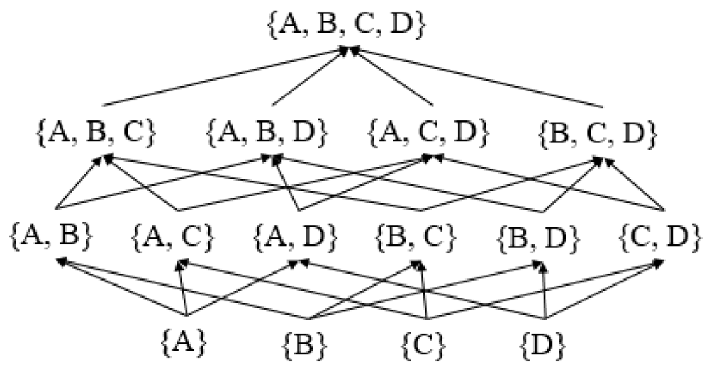
Figure 1. Nonempty combinations of attributes A, B, C, and D by k-level.

There are n · 2^n–1 – n = 4 · 2^4–1 – 4 = 28 edges (or arrows) in the semi-lattice of the complete search space for FDs in relation r(U) (Yao & Hamilton, 2008). The size of the search space for FDs is exponentially related to the number of attributes in U. Hence, the search space for FDs increases quite significantly when there is a greater number of attributes in U. For instance, when there are 12 attributes in a relation, the search space for FDs climbs to 24,564. This gives reason to be cautious of runtime and memory costs when deploying a rule mining algorithm to discover FDs.

Partition

The algorithms used to discover FDs differ in their approach to navigating the complete search space of a relation. Their candidate pruning methods vary and sometimes the methods used to validate FDs do as well. These differences affect runtime and memory behavior when used to process tables of different dimensions.

A common data structure used to validate FDs is the partition. A partition places tuples that have the same values on an attribute into the same group (Yao et al., 2002).

Definition 2. Let X ⊆ U and let t₁,…,t_n be all the tuples in a relation r(U). The partition over X, denoted ∏_X, is a set of the groups such that t_i and t_j, 1 ≤ i, j ≤ n, i 1≠ j, are in the same group if and only if t_i [X] = t_j [X] (Yao et al., 2002).

It follows from Definition 2 that the cardinality of the partition card(∏_A(r)) is the number of groups in partition ∏_A (Yao & Hamilton, 2008). The cardinality of the partition offers a quick approach to validating FDs in a dataset.

Theorem 1. An FD X → Y is satisfied by a relation r(U) if and only if card(∏_X) = card(∏_XY) (Huhtala et al., 1999).

Theorem 1 provides an efficient method to check whether an FD X → Y holds in a relation². Huhtala et al. (1999) proved it to support a fast validation method for relations consisting of a large number of tuples.

Closure

Efforts in relational database theory have lead to more runtime and memory efficient methods to check the complete search space of a relation for FDs. In place of needing each arrow in a semi-lattice checked, we can infer the FDs that logically follow from those already discovered. Such FDs are to be discovered as a consequence of Armstrong’s Axioms (Maier, 1983) and the inference axioms derivable from them (Ramakrishnan & Gehrke, 2000), which are

– Reflexivity: Y ⊆ X implies X → Y;
– Augmentation: X → Y implies XZ → YZ;
– Transitivity: X → Y and Y → Z imply X → Z;
– Union: X → Y and X → Z imply X → YZ;
– Decomposition: X → YZ implies that X → Y and X → Z.

These axioms signal the distinction between FDs that can be inferred from already discovered FDs and those that cannot (Maier, 1983). Exploiting what can be derived from Armstrong’s Axioms allows us to avoid having to check many of the candidates in a search space.

Definition 3. Let F be a set of functional dependencies over a dataset D and X be a candidate over D. The closure of candidate X with respect to F, denoted X⁺, is defined as {Y | X → Y can be deduced from F by Armstrong’s Axioms} (Yao & Hamilton, 2008).

The nontrivial closure³ of candidate X with respect to F is defined as X* = X⁺ \ X and written X* (Yao & Hamilton, 2008). Definition 3 gives room to elegantly define keys. Informally, a key implies that a relation does not have two distinct tuples with the same values on those attributes. Keys uniquely identify all tuple records.

Definition 4. Let R be a relational schema and X be a candidate of R over a dataset D. If X ∪ X* = R, then X is a key (Yao et al., 2002).

A candidate key X of a relation is a minimal key for that relation. This means that there is no proper subset of X for which Definition 4 holds.

Rule mining algorithms

Existing functional dependency algorithms are split between three categories: Difference- and agree-set algorithms (e.g., Dep-Miner, FastFDs), Dependency induction algorithms (e.g., FDEP), and Lattice traversal algorithms (e.g., TANE, FUN, FD_Mine, DFD) (Papenbrock et al., 2015).

Difference- and agree-set algorithms model the search space of a relation as the cross product of all tuple records (Papenbrock et al., 2015). They search for sets of attributes agreeing on the values of certain tuple pairs. Attribute sets only functionally determine other attribute sets whose tuple pairs agree, i.e., agree-sets (Asghar & Ghenai, 2015; Papenbrock et al., 2015). Then, agree-sets are used to derive all minimal FDs.

Dependency induction algorithms assume a base set of FDs in which each attribute functionally determines each other attribute (Papenbrock et al., 2015). While iterating through row data, observations are made that require certain FDs to be removed from the base set and others added to it. These observations are made by comparing tuple pairs based on the equality of their projections. After each record in a dataset is compared, the FDs left in the base set are considered valid, minimal and complete (Papenbrock et al., 2015).

Lattice traversal algorithms model the search space of a relation as a power set lattice. Most of such algorithms, (i.e., TANE, FUN, FD_Mine) use a level-wise approach to traversing the search space of a relation from the bottom-up (Papenbrock et al., 2015). They start by checking⁴ for FDs that are singleton sets on the left-hand side and iteratively transition to candidates of greater cardinality.

Performance

Papenbrock et al. (2015) released an experimental comparison of the aforementioned FD discovery algorithms. The seven algorithms were re-implemented in Java based on their original publications and applied to 17 datasets of various dimensions. They found that none of the algorithms are suited to yield the complete result set of FDs from a dataset consisting of 100 columns and 1 million rows (Papenbrock et al., 2015). Hence, it is a matter of discretion to choose the algorithm best fitting the dimensions of a dataset.

The experimental results show that lattice traversal algorithms are the least memory efficient, since each k-level⁵ can be a factor greater than the size of the previous level (Papenbrock et al., 2015). Difference- and agree-set algorithms and dependency induction algorithms perform favorably in memory experiments as a result of their operating directly on data and efficiently storing result sets. Lattice traversal algorithms scale poorly on tables with many columns (≥ 14 columns) due to memory limits (Papenbrock et al., 2015).

Lattice traversal algorithms are the most effective on datasets with many rows, because their validation method⁶ operates on attribute sets as opposed to data (Papenbrock et al., 2015). This puts such algorithms in a special position to rule mine clinical and demographic record datasets, which often consist of long and narrow sets of participant records. Difference- and agree-set algorithms and dependency induction algorithms commonly reach time limits when applied to datasets of these dimensions (> 100,000 rows) (Papenbrock et al., 2015).

Lattice traversal algorithms

Lattice traversal algorithms iterate through k-levels represented in a power set lattice. If the lattice is traversed from the bottom-up, we say the algorithm is level-wise.

Definition 5. Let X₁, X₂,…, X_k, X_k₊₁ be (k + 1) attributes over a database D. If X₁X₂… X_k → X_k₊₁ is an FD with k attributes on its left hand side, then it is called a k-level FD (Yao et al., 2002).

The search space for FDs is reduced at the end of each iteration using pruning rules. Pruning rules check the validity of candidates not yet checked with FDs already discovered and those inferred from Armstrong’s Axioms (Yao & Hamilton, 2008). After a search space is pruned, an Apriori_Gen principle generates k-level candidates with the (k – 1)-level candidates that were not pruned (Yao & Hamilton, 2008).

Apriori_Gen:

– oneUp: generates all possible candidates in C_k from those in C_k_–1.
– oneDown: generates all possible candidates in C_k_–1 from those in C_k.

Level-wise lattice traversal algorithms stop iterating after all candidates in a search space are pruned. In this case, Apriori_Gen generates the null set ∅ raising a flag for the algorithm to terminate. This has the effect of shortening runtime to the degree that FDs are discovered and others are inferred.

Tane

The level-wise lattice traversal algorithms TANE, FUN, and FD_Mine differ in terms of pruning rules. FUN and FD_Mine expand on the pruning rules of TANE. Released by Huhtala et al. (1999), TANE prunes a search space on the basis that only minimal and non-trivial⁷ FDs need be checked. TANE restricts the right-hand side candidates C⁺ for each attribute combination X to the set

C^{+} (X) = {A \in R | \forall B \in X : X \ {A, B} \to B does not hold},

which contains all the attributes that the set X may still functionally determine (Papenbrock et al., 2015). The set C⁺ is used in the following pruning rules (Papenbrock et al., 2015).

• Minimality pruning: If an FD X \ A → A holds, A and all B ∈ C⁺ (X) \ X can be removed from C⁺ (X).

• Right-hand side pruning: If C⁺ (X) = ∅, the attribute combination X can be pruned from the lattice, as there are no more right-hand side candidates for a minimal FD.

• Key pruning: If the attribute combination X is a key, it can be pruned from the lattice.

Key pruning implies that all supersets of a key, i.e., super keys, can be removed, since they are by definition non-minimal (Huhtala et al., 1999).

FD_Mine

Like TANE and FUN, FD_Mine is structured around the level-wise lattice traversal approach and the aforemented pruning rules. Unlike the other two algorithms, FD_Mine, authored by Yao et al. (2002), uses the concept of equivalence as means to more exhaustively prune the search space of a candidate (Papenbrock et al., 2015). Informally, attribute sets are equivalent if and only if they are functionally dependent on each other (Papenbrock et al., 2015).

The proofs demonstrating that no useful information is lost in pruning candidates from equivalent attribute sets are reproduced in this section and were originally developed by Yao & Hamilton (2008). The equivalence pruning method can be derived directly from Armstrong’s Axioms.

Definition 6. Let X and Y be candidates over a dataset D. If X → Y and Y → X hold, then we say that X and Y are an equivalence and denote it as X ↔ Y.

After a k-level is fully validated, i.e., each k-level candidate is checked, FD_Mine determines equivalent attribute sets with the FDs already discovered.

Theorem 2. Let X, Y ⊆ U. If Y ⊆ X⁺ and X ⊆ Y⁺, then X ↔ Y (Yao & Hamilton, 2008).

Proof. Since X → X⁺ and Y ⊆ X⁺, Decomposition implies that X → Y. By a similar argument, Y → X holds. Because X → Y and Y → X, we have by definition that X ↔ Y holds.

Lemma 3 and Lemma 4 are derived from Armstrong’s Axioms with the assumption of the equivalence X ↔ Y.

Lemma 3. Let W,X,Y,Y',Z ⊆ U and Y ⊆ Y'. If X ↔ Y and XW → Z, then Y'W → Z (Yao & Hamilton, 2008).

Proof. Suppose that X ↔ Y and XW → Z. This implies that X → Y. By Augmentation, YW → XW. By Transitivity, YW → XW and XW → Z give that YW → Z. By Augmentation, Y' \ Y can be added to both sides of YW → Z to give that YW(Y' \ Y) → Z(Y' \ Y). By Y ⊂ Y', we know that Y'W → Z(Y' \ Y). Then, by Decomposition, Y'W → Z.

Lemma 4. Let W,X,Y,Z ⊆ U. If X ↔ Y and WZ → X, then WZ → Y (Yao & Hamilton, 2008).

Proof. By X ↔ Y, we know that X → Y. By Transitivity, WZ → X and X → Y imply WZ → Y.

Theorem 2 checks attribute sets X and Y for the equivalence X ↔ Y. FD_Mine assumes that the attribute set Y is generated before X. By Lemma 3 and Lemma 4, we know that for equivalence X ↔ Y, no further attribute sets Z such that Y ⊆ Z need be checked (Yao & Hamilton, 2008). Hence, Y is deleted as a result of the following pruning rule.

• Equivalence pruning: If X ↔ Y is satisfied by relation r(U), then candidate Y can be deleted. (Yao & Hamilton, 2008).

Exploiting the equivalence pruning method leaves FD_Mine in a more aggressive position to prune candidates than TANE. This offers an advantage in terms of runtime and memory behavior (Yao et al., 2002).

Non-minimal FDs

The pseudo-code proposed in the second version of FD_Mine (Yao & Hamilton, 2008) will under certain circumstances output non-minimal FDs (Papenbrock et al., 2015). FD_Mine references an Apriori_Gen method (Agrawal et al., 1996) stating that for each pair of candidates p, q ∈ C_k_–1 the set p ∪ q is to be placed in C_k if card(p ∪ q) = k. Example 1 shows that the Apriori_Gen method referenced and utilized by FD_Mine can violate minimality pruning by checking supersets that need not be checked. Figure 2 gives the power set lattice of the relation described in Example 1 pruned by FD_Mine.

Figure 2. A pruned power set lattice.

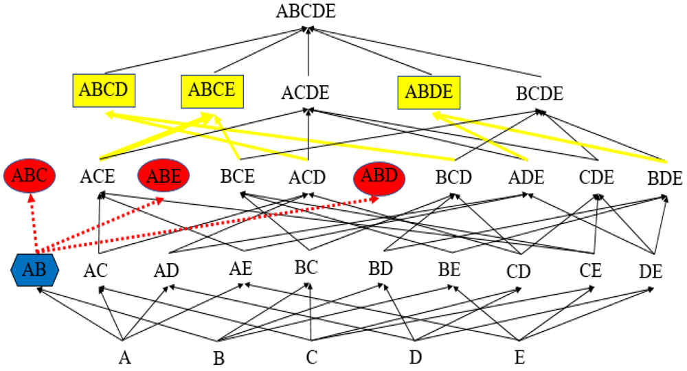
FD_Mine deletes the candidates ABC, ABE, and ABD (red ovals) as a result of finding the candidate key AB (blue hexagon). It generates supersets of AB (yellow rectangles) at the next level.

Example 1. Let r(U) be a relation such that U = {A,B,C,D,E}. Suppose that AB is a key and that there are no other FDs in r(U). Since AB is a key, we know by definition that AB ∪ AB* = U. Provided this and that there are no other FDs in r(U), the candidates ABC, ABD and ABE are deleted from C₃, and so C₃ = Prune(Apriori_Gen(C₂)) = {ACE, BCE, ACD, BCD, ADE, CDE, BDE}⁸. Then, C₄ = {ABCD, ABCE, ACDE, ABDE, BCDE}. Because it must be that AB* = {C, D, E}, the algorithm validates the FDs ABCD → E, ABCE → D, and ABDE → C. Since E, for example, is functionally dependent on the proper subset AB ⊆ ABCD, ABCD → E is non-minimal.

The Apriori_Gen principle presented in TANE (Huhtala et al., 1999) more effectively generates candidate level C_k₊₁ from C_k. It requires that C_k₊₁ only contains the attribute sets of size k + 1 which have all their subsets of size k in C_k (Huhtala et al., 1999); i.e.,

C_{k + 1} = {X | card (X) = k + 1 and for all ϒ with ϒ \subseteq X and card (ϒ) = k we have ϒ \in C_{k}} \cdot

In reference to Example 1, this method does not insert the candidate ABCD in C₄, without loss of generality, because ABC ⊆ ABCD but ABC ∉ C₃. Thus, the non-minimal FD ABCD → E is not checked.

Prune(C_k, E, Closure)^9–11

$\begin{array}{l} 01 for each S \in C_{k} : \\ 02 for each X \in o n e D o w n [C_{k}] : \\ 03 if (X \subset S) then: \\ 04 if (X \in {Z | ϒ \leftrightarrow Z \in E}) then: # Pruning rule 1 \\ 05 delete S from C_{k} \\ 06 if S \subset X^{+} then: # Pruning rule 2 \\ 07 delete S from C_{k} \\ 08 S^{+} = S^{+} \cup X^{*} # Pruning rule 3 \\ 09 if U == S^{+} then: # Pruning rule 4 \\ 10 delete S from C_{k} \\ 11 return C_{k}, C l o s u r e; \end{array}$

FD_Mine will under the circumstance described in Example 1 set closure values incorrectly. In line 2, FD_Mine iterates through C_k_–1, as opposed to oneDown [C_k], which can cause the Prune() function to ignore setting the closure values of certain candidates. In Example 1, FD_Mine does not accurately set the closure ABCD* to E, since E is not saved to the closure values of the candidates ACD, BCD ⊆ ABCD at the previous level. Iterating through oneDown [C_k] sets the closure of a candidate to the union of the closure values of its proper subsets, so that the closure values of deleted candidates are not lost among their supersets.

Properly assigned closure values can allow the algorithm to avoid checking many non-minimal FDs. This is because the ObtainFDs module, i.e., the validation method, only checks¹² the right-hand side attributes v_i for which v_i ∈ U \ X⁺ (Yao & Hamilton, 2008). Hence, provided that Pruning rule 3 asserts the equality ABCD* = E, ABCD → E need not be checked.

Operation

FDTool (Buranosky, 2018) is a command line Python application executed with the following statement: $ fdtool /path/to/file¹³. For Windows users, this is to be run from the directory in which the executable fdtool.exe resides, which will likely be C:\Python27\Scripts for those installing with pip install fdtool. For other systems, installation automatically inserts the file path to the fdtool command in the PATH variable. /path/to/file is the absolute or relative path to a .txt, .csv, or .pkl file containing a tabular dataset. If the data file has the extension .txt or .csv, FDTool detects the following separators: comma (‘,’), bar (‘|’), semicolon (‘;’), colon (‘:’), and tilde (‘∼’). The data is read in as a Pandas data frame₁₄.

Dependencies:

1. Python2 (https://www.python.org/), recommended version 2.7.8 or later.
2. Pandas data analysis library (https://pandas.pydata.org/) via: pip install pandas.

FDTool provides the user with the minimal FDs, equivalent attribute sets and candidate keys mined from a dataset. This is given with the time (s) it takes for the code to terminate (after reading in data), the row count and attribute count of the data, the number of FDs and equivalent attribute sets found, and the number of FDs checked. This is printed on the terminal after the code is executed as shown in Figure 3. The information is saved to a .FD_Info.txt file.

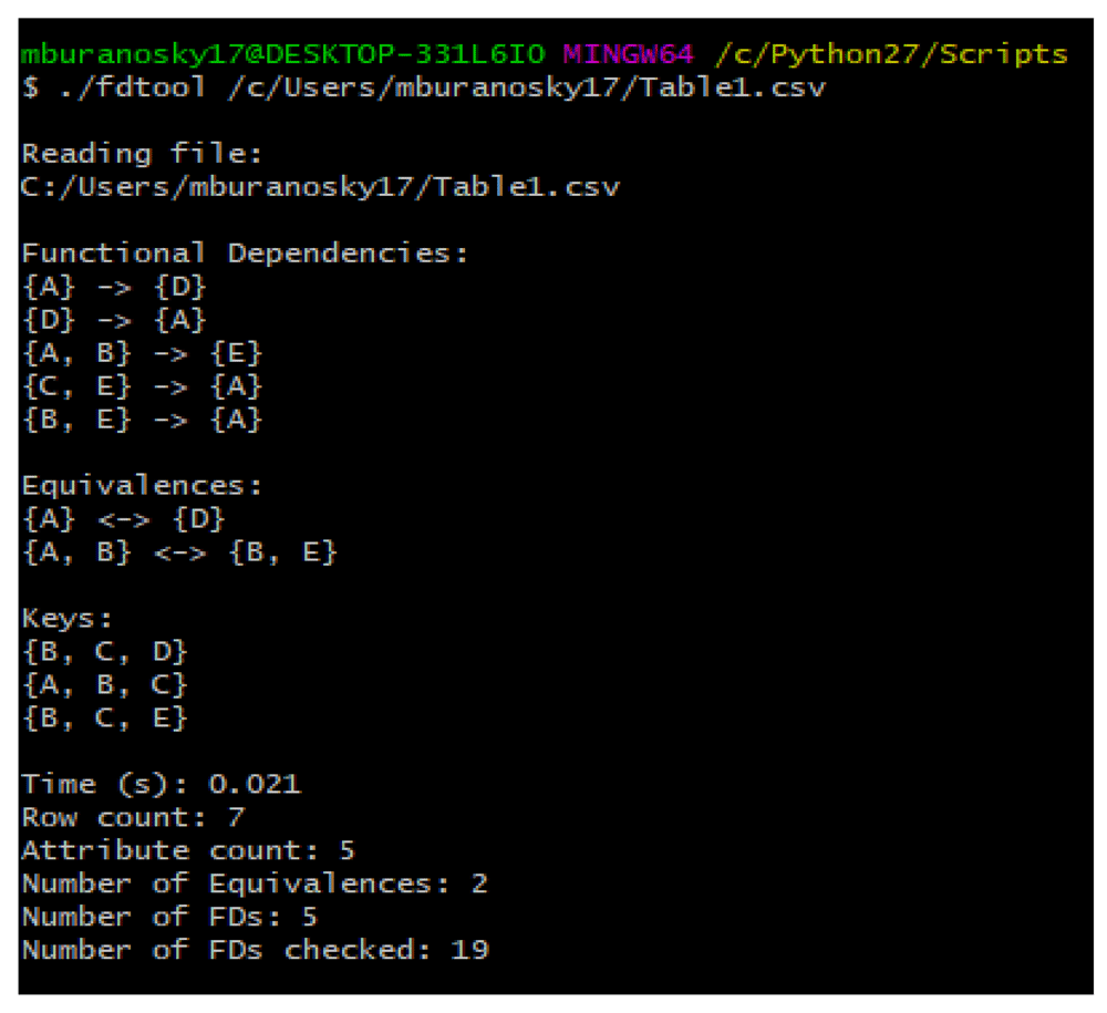
Figure 3. Printed output of FDTool.exe.

Figure 3 shows the printed output of FDTool.exe applied to the contents of Table 1. The output file Table1. FD_Info.txt is saved to the directory from which the executable is run.

Table 1.

A	B	C	D	E
0	0	0	2	0
0	1	0	2	0
0	2	0	2	2
0	3	1	2	0
4	1	1	1	4
4	3	1	1	2
0	0	1	2	0

Implementation

FDTool is a Python based re-implementation of the FD_Mine algorithm with additional features added to automate typical processes in database architecture. FD_Mine was published in two papers with more detail given to the scientific concepts used in algorithms of its kind (Yao et al., 2002; Yao & Hamilton, 2008). The two versions of FD_Mine were released with different structures but make use of the same theoretical foundation (Papenbrock et al., 2015), which is fully supported in mathematical proofs of the pruning rules used (Yao & Hamilton, 2008). FDTool was coded¹⁵ with special attention given to the pseudo-code presented in the second version of FD_Mine (Yao & Hamilton, 2008).

The Python script dbschema.py in FDTool/fdtool/modules/dbschema is taken from dbschemacmd (https://www.elstel.org/database/dbschemacmd.html.en): a tool for database schema normalization working on functional dependencies (Elmasri & Navathe, 2011). It is used to take sets of FDs and infer candidate keys from them. The operation first assigns the left-hand side attribute combinations of a set of FDs to dictionary keys and their closures to the corresponding values. It then reduces the set of FDs to a minimum coverage¹⁶. Candidate keys are assembled using the minimum coverage and closure structure by adding attributes to key candidates until each minimal attribute set X for which X⁺ = U is found. Details on the dbschema operations are described in FDTool/fdtool/modules/dbschema/Docs.

Use cases

FDTool was initially created to help decompose datasets of medical records as part of Clinical Archived Records research for Environmental Studies (CARES). CARES currently contains 12 datasets obtained from the medical software firms Epic and Legacy. The attribute count in this database ranges from 4 to 18; the row count ranges from 42,369 to 8,201,636.

Experimental results

To limit the strain on computational resources, FDTool has a built in time limit of 4 hours. FDTool reaches this preset limit (triggering program termination) when applied to the PatientDemographics dataset (42369 rows × 18 columns) and the EpicVitals_TobaccoAlcOnly dataset (896962 rows × 18 columns). The remaining 10 CARES datasets are given in Table 2¹⁷.

Table 2. Experimental results of FDTool on 10 CARES datasets, which terminate in less than 4 hours (preset limit)

Dataset Name	Attribute Count	Row Count	No. of FDs checked	No. of FDs found	No. of Equivalences	Time (s)
AllDxs	7	8201686	112	7	1	577.9
AllLabs	10	1294106	818	43	4	999.8
AllVisits	9	2019117	346	44	7	804.1
EpicMeds	10	1281731	453	26	0	551.9
EpicVitals2015	7	1246303	127	2	0	86.5
EpicVitals2016	7	988327	127	2	0	63.0
FamHx	4	93725	15	0	0	0.7
LegacyIPMeds	8	647122	79	14	1	28.2
LegacyOPMeds	7	740616	33	18	1	7.7
LegacyPayors	4	1465233	15	4	1	9.4
LegacyVitals	8	1453927	146	7	0	134.4

Experimental summary

The results from Table 2 show that runtime is primarily determined by the number of attributes in a dataset. For instance, the LegacyPayors dataset (1465233 rows × 4 columns) has slightly more rows (13% increase) but far fewer attributes (60% decrease) as compared to the AllLabs dataset (1294106 rows × 10 columns). The runtime of LegacyPayers (9.4 s.) is much less than that of AllLabs (999.8 s.), because AllLabs has many more arrows in its powerset lattice,

n . 2^{n - 1} - n = 10 . 2^{10 - 1} - 10 = 5110,

than does LegacyPayers (28). Hence, FDTool has more FDs to check when applied to AllLabs. It is clear that the attribute count of a dataset has a much greater effect on the runtime of FDTool than does row count.

Many of the arrows in the powerset lattice of a candidate are pruned by FDTool. AllLabs has 5110 arrows in its powerset lattice. However, FDTool only checks 818 FDs, as there are many inferred from the 43 FDs found. This follows from the Prune() function, which deletes many of the candidates to check partially as a result of mining 4 equivalent attribute sets. FDTool terminates after 5 k-levels when applied to AllLabs.

Future development

We want to improve its performance so that FDTool is better equipped to handle datasets of different dimensions. Using the dependency induction algorithm FDEP, the reach of FDTool could be extended to datasets with fewer rows and more than 100 columns (Papenbrock et al., 2015). This might also require upgrading the source code with multicore processing methods, such as a Java API, to reduce runtime and avoid reaching memory limits. A formal proof of the the dbschema operations is also desired.

Another goal is to increase the functionality provided by FDTool. This would mean implementing the pen and paper methods typically used to normalize relational schema and decompose tables. Our intent is to incorporate these changes in newer versions of FDTool, released at regular periods, so as to develop it as Python software that could automate much of what is done in the database design process.

Data availability

While the authors fully support the open dissemination of data for verification and replication purposes, CARES data cannot be released as it contains Protected Health Information. However, the CARES data is accessible to any researcher who has an approved IRB and submits a data request to the Carolina Data Warehouse for Health (https://tracs.unc.edu/index.php/services/informatics-and-data-science/cdwh; use the “Submit a CDW-H Project Data Request” link). The authors will be happy to send the CARES data exactly as utilized in this manuscript to any researcher with an approved request from the Carolina Data Warehouse for Health.

Software availability

FDTool is available from the Python Package Index: https://pypi.org/project/fdtool/

Latest source code: https://github.com/USEPA/FDTool.git

Source code at time of publication: https://zenodo.org/record/1442843

License: CC0 1.0 Universal. Module FDTool/fdtool/modules/dbschema released under a modified C-FSL license.

Author contributions

MB and ES designed and implemented the software. MB wrote the manuscript. CWC supervised MB, and reviewed the manuscript. EP maintained the research data. DDS coordinated the funding for the project. All authors agreed to the final content of the manuscript.

Grant information

This work was funded by the US Environmental Protection Agency. The work presented here does not necessarily reflect the views or policy of the EPA. Any mention of trade names does not constitute endorsement by the EPA.

The funders had no role in study design, data collection and analysis, decision to publish, or preparation of the manuscript.

Footnotes

¹Each attribute v_i has a finite domain, written dom(v_i), representing the values that v_i can take on. For a subset X = {v_i,…,v_j} of U, we write dom(X) for the Cartesian product of the domains of the individual attributes in X, namely, dom(X) = dom(v_i) × … × dom(v_j) (Yao & Hamilton, 2008). A relation r on U, denoted r(U), is a finite set of mappings {t₁,…,t_n} from U to dom(U) with the restriction that for each mapping t ∈ r(U), t[v_i] must be in dom(v_i), 1 ≤ i ≤ m, where t[v_i] denotes the value obtained by restricting the mapping t to v_i. Each mapping t is called a tuple and t(v_i) is called the v_i-value of t (Maier, 1983).

²FDTool uses Theorem 1 as means to check FDs in the GetFDs module with the pandas data analysis library functions nunique() and dropduplicates.count().

³FDTool saves the closure of candidates at each level before releasing it from memory at levels that follow.

⁴ We say that an FD is checked when Theorem 1 is used to see if it holds or not (Yao et al., 2002).

⁵Definition 5.

⁶Theorem 1.

⁷An FD X → A is non-trivial if and only if X ∉ A (Huhtala et al., 1999).

⁸Since E = ∅ in this example, we can ignore the argument E in the function Prune(). For simplicity’s sake, we ignore the argument Closure.

⁹Closure = {X⁺ | X ∈ C_k V X ∈ oneDown [C_k]}.

¹⁰Equivalent candidates are stored in E.

¹¹All candidates at level k are stored in C_k.

¹² Assume the left-hand side attribute set X.

¹³Edit FDTool/fdtool/config.py prior to building setup with python setup.py install to change preset time limit or max k-level.

¹⁴The data is read in with the Pandas function read_csv(), which is subject to the usual spacing errors associated with reading in delimiter-separated values.

¹⁵FDTool was tested regularly throughout the implementation process so as to accomodate to changes made to improve runtime and memory behavior.

¹⁶A set of FDs F is a coverage of another set of FDs G if every FD in G can be inferred from F; i.e., G⁺ ⊆ F⁺ (Soule, 2014). F is a minimum coverage of G if F is the smallest set of FDs that covers G (Soule, 2014).

¹⁷OS: Windows 10; Installed memory (RAM): 256 GB; Processor: Intel Core, 1 CPU; Clock speed: 2.19 GHz; Python: 2.7.12; Pandas: 0.18.1.

Faculty Opinions recommended

References

Agrawal R, Mannila H, Srikant R, et al.: Fast discovery of association rules. Advances in knowledge discovery and data mining. 1996; 12(1): 307–328. Reference Source
Asghar N, Ghenai A: Automatic discovery of functional dependencies and conditional functional dependencies: A comparative study. 2015. Reference Source
Buranosky M: USEPA/FDTool: FDTool (Version v0.1.7). Zenodo. 2018. http://www.doi.org/10.5281/zenodo.1442843
Elmasri R, Navathe SB: Database Systems: Models, Languages, Design, and Application Programming. Pearson. 2011. Reference Source
Huhtala Y, Kärkkäinen J, Porkka P, et al.: Tane: An efficient algorithm for discovering functional and approximate dependencies. Comput J. 1999; 42(2): 100–111. Publisher Full Text
Maier D: Theory of Relational Databases. Computer Science Pr. 1983. Reference Source
Papenbrock T, Ehrlich J, Marten J, et al.: Functional dependency discovery: An experimental evaluation of seven algorithms. Proc VLDB Endow. 2015; 8(10): 1082–1093. Publisher Full Text
Ramakrishnan R, Gehrke J: Database Management Systems. McGraw-Hill, Inc., New York, NY, USA, 2nd edition, 2000. Reference Source
Soule R: Functional dependencies and finding a minimal cover. 2014. Reference Source
Yao H, Hamilton HJ: Mining functional dependencies from data. Data Min Knowl Discov. 2008; 16(2): 197–219. Publisher Full Text
Yao H, Hamilton H, Butz C: Fd_mine: Discovering functional dependencies in a database using equivalences. 2002. Publisher Full Text

Comments on this article Comments (0)

Version 2

VERSION 2 PUBLISHED 19 Oct 2018

Author details Author details

¹ National Health and Environmental Effects Research Laboratory, United States Environmental Protection Agency, Chapel Hill, NC, USA
² University of Klagenfurt, Klagenfurt, Austria
³ University of North Carolina at Chapel Hill, Chapel Hill, NC, USA

Matt Buranosky
Roles: Software, Writing – Original Draft Preparation

Elmar Stellnberger
Roles: Software

Emily Pfaff
Roles: Data Curation

David Diaz-Sanchez
Roles: Funding Acquisition

Cavin Ward-Caviness
Roles: Supervision, Writing – Review & Editing

Competing interests

No competing interests were disclosed.

Grant information

This work was funded by the US Environmental Protection Agency. The work presented here does not necessarily reflect the views or policy of the EPA. Any mention of trade names does not constitute endorsement by the EPA.
The funders had no role in study design, data collection and analysis, decision to publish, or preparation of the manuscript.

Article Versions (2)

version 2

Revised

Published: 19 Jun 2019, 7:1667

https://doi.org/10.12688/f1000research.16483.2

version 1

Published: 19 Oct 2018, 7:1667

https://doi.org/10.12688/f1000research.16483.1

Copyright

© 2018 Buranosky M et al. This is an open access article distributed under the terms of the Creative Commons Attribution License, which permits unrestricted use, distribution, and reproduction in any medium, provided the original work is properly cited.

Download

Export To

metrics

	Views	Downloads
F1000Research	-	-
PubMed Central Data from PMC are received and updated monthly.	-	-

Citations

0

SEE MORE DETAILS

CITE

how to cite this article

Buranosky M, Stellnberger E, Pfaff E et al. FDTool: a Python application to mine for functional dependencies and candidate keys in tabular data [version 1; peer review: 2 approved]. F1000Research 2018, 7:1667 (https://doi.org/10.12688/f1000research.16483.1)

NOTE: If applicable, it is important to ensure the information in square brackets after the title is included in all citations of this article.

track

receive updates on this article

Track an article to receive email alerts on any updates to this article.

Open Peer Review

Version 1

VERSION 1

PUBLISHED 19 Oct 2018

Views

19

Reviewer Report 29 Apr 2019

Sayan Mukherjee, Department of Statistical Science, Duke University, Durham, NC, USA

Approved

https://doi.org/10.5256/f1000research.18017.r46574

This paper outlines in detail FDTool: a Python application to mine for functional dependencies. The paper is about developing a database tool that improves FD Mine a previous tool for functional dependencies

The definitions, problem statement and explanations ... Continue reading

This paper outlines in detail FDTool: a Python application to mine for functional dependencies. The paper is about developing a database tool that improves FD Mine a previous tool for functional dependencies

The definitions, problem statement and explanations in this paper are well written and clear. The authors also provide a good comparison of several functional dependence discovery algorithms.

In my opinion, it would be nice to have the experimental results and summary in some more detail. Also since the CARES data is not public it would be nice to have some results on available data.

Is the rationale for developing the new software tool clearly explained?

Yes
Is the description of the software tool technically sound?

Yes
Are sufficient details of the code, methods and analysis (if applicable) provided to allow replication of the software development and its use by others?

Partly
Is sufficient information provided to allow interpretation of the expected output datasets and any results generated using the tool?

Yes
Are the conclusions about the tool and its performance adequately supported by the findings presented in the article?

Yes

Competing Interests: No competing interests were disclosed.

Reviewer Expertise: Statistical and computation methods.a

I confirm that I have read this submission and believe that I have an appropriate level of expertise to confirm that it is of an acceptable scientific standard.

CITE

Report a concern

Respond or Comment

Views

33

Reviewer Report 10 Dec 2018

Howard J. Hamilton, Department of Computer Science, University of Regina, Regina, SK, Canada

Shubhashis Shil, University of Regina, Regina, SK, Canada

Approved

https://doi.org/10.5256/f1000research.18017.r39685

The article is well-structured and well-written. It contains nice presentations of appropriate definitions, theorems, algorithms, examples, and use-cases.

The article has clear contributions:

In the theory part: It enhances the FD_Mine algorithm by improving ... Continue reading

The article is well-structured and well-written. It contains nice presentations of appropriate definitions, theorems, algorithms, examples, and use-cases.

The article has clear contributions:

In the theory part: It enhances the FD_Mine algorithm by improving performance and automating typical processes.

In the implementation part: The authors re-implement the FD_Mine algorithm, which is otherwise not publicly available as a software tool.

In the experiment part: The authors apply FDTool to 12 datasets of different dimensions.

Findings: The effect of the attributes is greater than the records on the runtime and memory costs of the FDTool.

Additional contributions:

The article clearly describes the features of the FDTool, such as its usage and execution. It also depicts future research opportunities with respect to the further development of the FDTool.

Major Comment:

In the abstract, it says, “We conclude that FD_Mine is the most efficient FD discovery algorithm when applied to datasets with many rows (> 100,000 rows) and few columns (< 14 columns).” The word “conclude” does not seem appropriate here. If this result indeed follows from your research, please explain how the results shown in Table 2 support this claim with respect to all datasets shown in the table [This explanation could be added in the experimental results or experimental summary section]. However, if the conclusion is in fact being taken from Papenbrock, then wording might be adjusted to “Previous research established that FD_Mine ….” You may want to state your conclusions about your software tool.

Minor corrections:

Please use either "FD_Mine" or "FD Mine" everywhere. The original paper had FD_Mine.

Please use same format (comma or no comma) for large numbers [e.g. “the row count ranges from 42,369 to 8,201,636” in the use cases section versus “AllLabs dataset (1294106” and “AllLabs has 5110 arrows in its powerset lattice” in the experimental summary]. Also please check the experimental results section.

In Definition 2, please correct “i 1≠ j”, presumably to “i ≠ j”.

In the text immediately after Definition 6, please change “determines equivalent attribute sets with” to “determines attribute sets equivalent to”.

In the first line of the closure section, please change “lead” to “led”.

In the future development section, please remove the extra "the" from "A formal proof of the the dbschema operations is also desired".

Table 1 has no title. Please give a title for Table 1.

Table 2 shows 11 datasets but the table title [and the description in the experimental results section] mentions 10 datasets. Could you please correct this inconsistency.

Is the rationale for developing the new software tool clearly explained?

Yes
Is the description of the software tool technically sound?

Yes
Are sufficient details of the code, methods and analysis (if applicable) provided to allow replication of the software development and its use by others?

Yes
Is sufficient information provided to allow interpretation of the expected output datasets and any results generated using the tool?

Yes
Are the conclusions about the tool and its performance adequately supported by the findings presented in the article?

Partly

Competing Interests: No competing interests were disclosed.

Reviewer Expertise: knowledge discovery, data mining, machine learning

We confirm that we have read this submission and believe that we have an appropriate level of expertise to confirm that it is of an acceptable scientific standard.

CITE

Report a concern

Respond or Comment

Comments on this article Comments (0)

Version 2

VERSION 2 PUBLISHED 19 Oct 2018

Open Peer Review

Reviewer Status

Reviewer Reports

	Invited Reviewers
	1	2
Version 2 (revision) 19 Jun 19
Version 1 19 Oct 18	read	read

Howard J. Hamilton, University of Regina, Regina, Canada

Shubhashis Shil, University of Regina, Regina, Canada
Sayan Mukherjee, Duke University, Durham, USA

Comments on this article

All Comments(0)

Add a comment

Sign up for content alerts

Browse by related subjects

Back to all reports

Reviewer Report

19 Views

29 Apr 2019 | for Version 1

Sayan Mukherjee, Department of Statistical Science, Duke University, Durham, NC, USA

19 Views Cite this report Responses(0)

Approved

This paper outlines in detail FDTool: a Python application to mine for functional dependencies. The paper is about developing a database tool that improves FD Mine a previous tool for functional dependencies

The definitions, problem statement and explanations in this paper are well written and clear. The authors also provide a good comparison of several functional dependence discovery algorithms.

In my opinion, it would be nice to have the experimental results and summary in some more detail. Also since the CARES data is not public it would be nice to have some results on available data.

Is the rationale for developing the new software tool clearly explained?

Yes
Is the description of the software tool technically sound?

Yes
Are sufficient details of the code, methods and analysis (if applicable) provided to allow replication of the software development and its use by others?

Partly
Is sufficient information provided to allow interpretation of the expected output datasets and any results generated using the tool?

Yes
Are the conclusions about the tool and its performance adequately supported by the findings presented in the article?

Yes

Competing Interests

No competing interests were disclosed.

Reviewer Expertise

Statistical and computation methods.a

I confirm that I have read this submission and believe that I have an appropriate level of expertise to confirm that it is of an acceptable scientific standard.

Respond to this report

Responses (0)

Back to all reports

Reviewer Report

33 Views

10 Dec 2018 | for Version 1

Howard J. Hamilton, Department of Computer Science, University of Regina, Regina, SK, Canada

Shubhashis Shil, University of Regina, Regina, SK, Canada

33 Views Cite this report Responses(0)

Approved

The article is well-structured and well-written. It contains nice presentations of appropriate definitions, theorems, algorithms, examples, and use-cases.

The article has clear contributions:

In the theory part: It enhances the FD_Mine algorithm by improving performance and automating typical processes.

In the implementation part: The authors re-implement the FD_Mine algorithm, which is otherwise not publicly available as a software tool.

In the experiment part: The authors apply FDTool to 12 datasets of different dimensions.

Findings: The effect of the attributes is greater than the records on the runtime and memory costs of the FDTool.

Additional contributions:

The article clearly describes the features of the FDTool, such as its usage and execution. It also depicts future research opportunities with respect to the further development of the FDTool.

Major Comment:

In the abstract, it says, “We conclude that FD_Mine is the most efficient FD discovery algorithm when applied to datasets with many rows (> 100,000 rows) and few columns (< 14 columns).” The word “conclude” does not seem appropriate here. If this result indeed follows from your research, please explain how the results shown in Table 2 support this claim with respect to all datasets shown in the table [This explanation could be added in the experimental results or experimental summary section]. However, if the conclusion is in fact being taken from Papenbrock, then wording might be adjusted to “Previous research established that FD_Mine ….” You may want to state your conclusions about your software tool.

Minor corrections:

Please use either "FD_Mine" or "FD Mine" everywhere. The original paper had FD_Mine.

Please use same format (comma or no comma) for large numbers [e.g. “the row count ranges from 42,369 to 8,201,636” in the use cases section versus “AllLabs dataset (1294106” and “AllLabs has 5110 arrows in its powerset lattice” in the experimental summary]. Also please check the experimental results section.

In Definition 2, please correct “i 1≠ j”, presumably to “i ≠ j”.

In the text immediately after Definition 6, please change “determines equivalent attribute sets with” to “determines attribute sets equivalent to”.

In the first line of the closure section, please change “lead” to “led”.

In the future development section, please remove the extra "the" from "A formal proof of the the dbschema operations is also desired".

Table 1 has no title. Please give a title for Table 1.

Table 2 shows 11 datasets but the table title [and the description in the experimental results section] mentions 10 datasets. Could you please correct this inconsistency.

Is the rationale for developing the new software tool clearly explained?

Yes
Is the description of the software tool technically sound?

Yes
Are sufficient details of the code, methods and analysis (if applicable) provided to allow replication of the software development and its use by others?

Yes
Is sufficient information provided to allow interpretation of the expected output datasets and any results generated using the tool?

Yes
Are the conclusions about the tool and its performance adequately supported by the findings presented in the article?

Partly

Competing Interests

No competing interests were disclosed.

Reviewer Expertise

knowledge discovery, data mining, machine learning

We confirm that we have read this submission and believe that we have an appropriate level of expertise to confirm that it is of an acceptable scientific standard.

Respond to this report

Responses (0)

[1] Agrawal R, Mannila H, Srikant R, et al.: Fast discovery of association rules. Advances in knowledge discovery and data mining. 1996; 12(1): 307–328. Reference Source

[2] Asghar N, Ghenai A: Automatic discovery of functional dependencies and conditional functional dependencies: A comparative study. 2015. Reference Source

[3] Buranosky M: USEPA/FDTool: FDTool (Version v0.1.7). Zenodo. 2018. http://www.doi.org/10.5281/zenodo.1442843

[4] Elmasri R, Navathe SB: Database Systems: Models, Languages, Design, and Application Programming. Pearson. 2011. Reference Source

[5] Huhtala Y, Kärkkäinen J, Porkka P, et al.: Tane: An efficient algorithm for discovering functional and approximate dependencies. Comput J. 1999; 42(2): 100–111. Publisher Full Text

[6] Maier D: Theory of Relational Databases. Computer Science Pr. 1983. Reference Source

[7] Papenbrock T, Ehrlich J, Marten J, et al.: Functional dependency discovery: An experimental evaluation of seven algorithms. Proc VLDB Endow. 2015; 8(10): 1082–1093. Publisher Full Text

[8] Ramakrishnan R, Gehrke J: Database Management Systems. McGraw-Hill, Inc., New York, NY, USA, 2nd edition, 2000. Reference Source

[9] Soule R: Functional dependencies and finding a minimal cover. 2014. Reference Source

[10] Yao H, Hamilton HJ: Mining functional dependencies from data. Data Min Knowl Discov. 2008; 16(2): 197–219. Publisher Full Text

[11] Yao H, Hamilton H, Butz C: Fd_mine: Discovering functional dependencies in a database using equivalences. 2002. Publisher Full Text

FDTool: a Python application to mine for functional dependencies and candidate keys in tabular data

Abstract

Keywords

Introduction

Power set lattice

Figure 1. Nonempty combinations of attributes A, B, C, and D by k-level.

Partition

Closure

Rule mining algorithms

Performance

Lattice traversal algorithms

Tane

FD_Mine

Non-minimal FDs

Figure 2. A pruned power set lattice.

Operation

Figure 3. Printed output of FDTool.exe.

Table 1.

Implementation

Use cases

Experimental results

Table 2. Experimental results of FDTool on 10 CARES datasets, which terminate in less than 4 hours (preset limit)

Experimental summary

Future development

Data availability

Software availability

Author contributions

Grant information

Footnotes

References

Comments on this article Comments (0)

Open Peer Review

Comments on this article Comments (0)

Open Peer Review

Reviewer Status

Reviewer Reports

Comments on this article

Browse by related subjects

Competing Interests Policy

Stay Updated