Keywords
orthologs, paralogs, hierarchical orthologous groups, comparative genomics, orthologous matrix, oma, API, R, python, REST, bioconductor
This article is included in the RPackage gateway.
This article is included in the Bioconductor gateway.
This article is included in the University College London collection.
This article is included in the Python collection.
This article is included in the The OMA collection collection.
orthologs, paralogs, hierarchical orthologous groups, comparative genomics, orthologous matrix, oma, API, R, python, REST, bioconductor
Version 2 of our manuscript addresses the points from the peer-reviewers, whom we thank for their constructive feedback.
We clarified the installation procedure for the package, which is currently in the development version of Bioconductor, due to be released in Spring 2019. Furthermore, we corrected typos, improved the documentation, and clarified potential differences in the output of the code examples that can arise due to updates of the OMA database.
See the authors' detailed response to the review by Laurent Gatto
See the authors' detailed response to the review by Bastian Greshake Tzovaras and Ngoc-Vinh Tran
Orthologs are pairs of protein coding genes that have common ancestry and have diverged due to speciation events1. The detection of orthologs is of fundamental importance in many fields in biology, such as comparative genomics, as it allows us to propagate existing biological knowledge to ever growing newly sequenced data2,3.
The Orthologous Matrix (OMA) is a method and resource for the inference of orthologs among complete genomes4. The OMA database (https://omabrowser.org) features broad scope and size with currently over 2,100 species from all three domains of life.
The OMA browser has supported multiple ways of exporting the underlying data from its beginning. Users can download data either via bulk archives or interactively through the browser—using where possible standard file formats, such as FASTA, OrthoXML5, or PhyloXML6. For programmatic access, early OMA database releases offered an Application Programming Interface (API) in the form of the Simple Object Access Protocol (SOAP). However, the complexity and limited adoption of SOAP has prompted us to recently switch to the simpler, faster, and more widely used Representational State Transfer (REST) protocol for the OMA API4. Here, we provide a description of this new OMA REST API.
Furthermore, the R environment is widely used in bioinformatics due to its flexibility as a high-level scripting language, statistical capabilities, and numerous bioinformatics libraries. In particular, the Bioconductor open source framework contains over 2,000 packages to facilitate either access to or manipulation of biological data7. This motivated us to develop the OmaDB Bioconductor package which provides a more idiomatic and user-friendly access to OMA data in R implemented on top of the REST API.
Finally, to also enable Python users to easily interact with the database, we have developed a similar package in that language, compliant with the conventions and with support of typical complementary Python packages as outlined below.
We start by describing the OMA REST API, before moving on to detail the OmaDB Bioconductor package, and finally outline the omadb Python package.
The REST framework is an API architectural style that is based on URLs and HTTP protocol methods. It was designed to be stateless and thus is context independent. That is, it does not save data internally between the HTTP requests which minimises server-side application state, thus easing parallelism. The combination of the HTTP and JSON data formats makes it particularly suitable for web applications and easily supported by most programming languages.
Since the backend of the OMA browser is almost fully based on Python and its frontend is supported by the Django web framework8, we have opted to use the Django Rest Framework (DRF) to implement a REST API in our latest release4. Most API calls require querying the OMA database, stored in HDF59, using a custom Python library (“pyoma”). The query results are serialised in the format requested by the user — typically JSON.
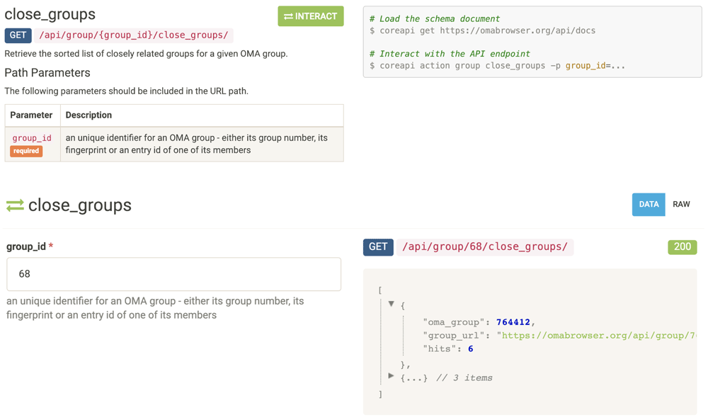
Most data available through the OMA browser is now also accessible via the API, with the exception of the local synteny data. This includes individual genes and their attributes such as protein or cDNA sequences, cross-references, pairwise orthologs, hierarchical orthologous groups10, as well as species trees and the corresponding taxonomy. The API documentation as well as the interactive interface can be found at https://omabrowser.org/api/docs (Figure 1).
To facilitate simplified access to the API and downstream analyses in the R environment, we have also developed an API wrapper package in R, now available in Bioconductor7 (http://bioconductor.org/packages/OmaDB/). This allowed for abstraction of the server interface, eliminating the need to know structure of the database or the URL endpoints to access the required data.
The package consists of a collection of functions that import OMA data into R objects, the type of which depends on the query supplied. Due to the volume of the data available, some selected object attributes are at first given as URL endpoints. However, these are automatically loaded upon accession. OmaDB also facilitates further downstream analyses with other Bioconductor packages, such as GO enrichment analysis with topGO11, sequence analysis with BioStrings12, phylogenetic analyses using ggtree13 or gene locus analyses with the help of GenomicRanges14.
The open source code is hosted at https://github.com/DessimozLab/OmaDB/. In the results section we showcase usage of the latest version of the package (v2.0), which requires R version >= 3.6 and Bioconductor version >= 3.9. Note that as of the time of publication, this is in the Bioconductor development version. For details, see the Software Availability section.
Package Installation
if (!requireNamespace("BiocManager"))
    install.packages("BiocManager")
BiocManager::install("OmaDB")
# Load the package
library(OmaDB)
For Python users, we provide an analogous package named omadb. Results are supplied to users as a hybrid attribute-dictionary object. As such, both attribute and key-based access is possible. Where the URL of a further API call is listed in a response, this has been designed to be automatically requested for the user.
For data that can be represented as a table, the pandas package15 is supported. HOGs can be analysed or displayed using the pyham library16. Trees are retrievable as DendroPy17 or ETE318 Tree objects. Gene Ontology enrichment analyses are possible through the use of the goatools package19.
The open source code is hosted at https://github.com/DessimozLab/pyomadb/. The package requires Python >=3.6, as well as a stable internet connection. It is also available to download from PyPI, installable using pip.
Package Installation
# Install in shell, using pip
$ pip install omadb

# In Python, load the package
>>> from omadb import Client
# Initialise the client
>>> c = Client()
We provide six illustrative examples in R. The first shows a direct call to the REST API, while the other five showcase the OmaDB R package (version 2.0). These examples are also available as a Jupyter notebook20 as part of the OmaDB R code repository. We have also provided analogous examples in Python, also in the form of a Jupyter notebook, included in its code repository—with the exception of Example 6, which uses a package only available in R.
Note that the results of the queries using the API and the packages may change as we continue to update the OMA database. The OMA database release of June 2018 was used to generate the examples below.
One way to access the API is to directly send a request using httr21 in R. This approach requires the user to know the URL of the API endpoint, as well as the URL of the API function of interest. Some additional processing steps of the resultant response is usually needed. A simple example to retrieve information on the P53_RAT protein is provided below.
Here we first formulate our URL of interest and use it to send a GET request to the API. This gives us the response JSON object, which can then be parsed into an R list.
library(httr)

url <- "https://omabrowser.org/api/protein/P53_RAT/"
response <- GET(url)

response_content_list <- httr::content(response, as = "parsed")
Below is a simple workflow using the OmaDB package to annotate a given protein sequence, using the mapSequence() function.
library(OmaDB)

sequence <- 'MKLVFLVLLFLGALGLCLAGRRRSVQWCAVSQPEATKCFQWQRNMRKVRGPPVSCIKRD
SPIQCIQAIAENRADAVTLDGGFIYEAGLAPYKLRPVAAEVYGTERQPRTHYYAVAVVKKGGSFQLNELQGL
KSCHTGLRRTAGWNVPIGTLRPFLNWTGPPEPIEAAVARFFSASCVPGADKGQFPNLCRLCAGTGENKCAFS
SQEPYFSYSGAFKCLRDGAGDVAFIRESTVFEDLSDEAERDEYELLCPDNTRKPVDKFKDCHLARVPSHAVV
ARSVNGKEDAIWNLLRQAQEKFGKDKSPKFQLFGSPSGQKDLLFKDSAIGFSRVPPRIDSGLYLGSGYFTAI
QNLRKSEEEVAARRARVVWCAVGEQELRKCNQWSGLSEGSVTCSSASTTEDCIALVLKGEADAMSLDGGYVY
TAGKCGLVPVLAENYKSQQSSDPDPNCVDRPVEGYLAVAVVRRSDTSLTWNSVKGKKSCHTAVDRTAGWNIP
MGLLFNQTGSCKFDEYFSQSCAPGSDPRSNLCALCIGDEQGENKCVPNSNERYYGYTGAFRCLAENAGDVAF
VKDVTVLQNTDGNNNEAWAKDLKLADFALLCLDGKRKPVTEARSCHLAMAPNHAVVSRMDKVERLKQVLLHQ
QAKFGRNGSDCPDKFCLFQSETKNLLFNDNTECLARLHGKTTYEKYLGPQYVAGITNLKKCSTSPLLEACEF
LRK'

seq_annotation <- mapSequence(sequence)
length(seq_annotation$targets)                               # 1
The identified targets can be found in the seq_annotation$targets. As the length of this object attribute is 1, in this example the sequence mapping identified a single target sequence. From this object further information can be obtained as follows:
seq_annotation$targets[[1]]$canonicalid # 'TRFL_HUMAN'
Thus, our sequence is human lactotransferrin (also known as lactoferrin). Lactotransferrin is one of four subfamilies of transferrins in mammals22.
To investigate the evolutionary history of genes more precisely, we turn to Hierarchical Orthologous Groups (HOGs)—sets of genes which have descended from a single common ancestral gene within a taxonomic range of interest10. For an introduction to HOGs, we refer the interested reader to the following short video: https://youtu.be/5p5x5gxzhZA.
By knowing the ID of the HOG to which our sequence belongs, we can obtain a list of all the HOG members (i.e. all genes in the HOG), as follows:
hog_id <- seq_annotation$targets[[1]]$oma_hog_id   # 'HOG:0413862.1a.1b'
hog <- getHOG(id = hog_id, members = TRUE, level = 'Mammalia')
hog$members
Note that it is also possible to access information on a HOG using the getHOG() function. A HOG can be identified by its ID or the ID of one of its member proteins. Therefore the below will produce the same output.
hog <- getHOG(id = 'TRFL_HUMAN', members = TRUE, level = 'Mammalia')
We can easily retrieve the Gene Ontology (GO) terms23 that are associated to each of the members using OmaDB.
go_annotations <- getProtein(hog$members$omaid,
    attribute = 'gene_ontology')
The resultant list of GO terms per gene is in the “geneID2GO” format by default, which is used by the topGO11 package.
To compare the function of lactotransferrins with their paralogous counterparts, we can retrieve a background set consisting of all members of the transferring HOG defined at the root of the eukaryotes
bgHOG <- getHOG(id = 'TRFL_HUMAN', members = TRUE, level = 'Eukaryota')
bgAnnnot <- getProtein(bgHOG$members$omaid, attribute = 'gene_ontology')
We can now construct a topGO object using the getTopGO function as seen below. Note that the background set of terms is set by getTopGO to all terms appearing in the list of annotations. This may not be appropriate in all cases—the choice of background set requires careful consideration24.
bgAnnnotFormatted = formatTopGO(bgAnnnot, format = 'geneID2GO')

library(topGO)
myGO <- getTopGO(annotations = bgAnnnotFormatted, format = 'geneID2GO',
     foregroundGenes = hog$members$entry_nr, ontology = 'BP')

myRes <- runTest(myGO, algorithm = 'classic', statistic = 'fisher')
print(GenTable(myGO, myRes))
As the output in Table 1 indicates, several enriched terms in the mammalian lactotransferrin are related to bone formation, consistent with previous reports in the literature (e.g. 25). So is the role of lactotransferrin in antimicrobial activity (e.g. 26).
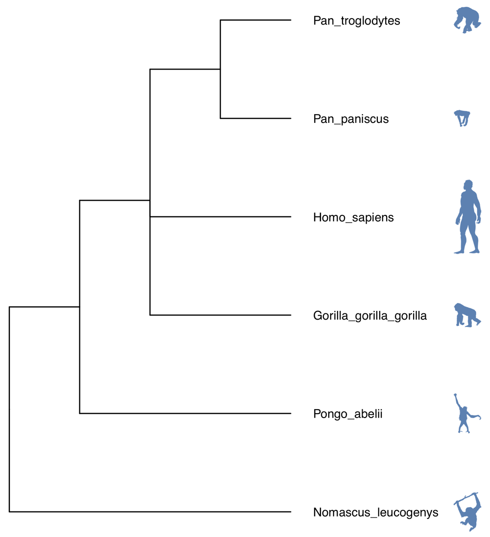
The taxonomic data obtained using the OmaDB package can easily be plugged into ggtree13 for phylogenetic tree visualisation. First, the tree is obtained using the getTaxonomy() function. In this example, the tree is rooted at the Hominoidea taxonomic level. The default format of the object returned is newick.
tax <- getTaxonomy(root = 'Hominoidea')
The resultant object can directly be used to build a phylogenetic tree using the ggtree package as below:
library(ggtree)
tree <- getTree(tax$newick)

mytree <- ggtree(tree)
The tree can be further annotated using species silhouettes from PhyloPic (http://phylopic.org/). This functionality is already enabled within the ggtree package and just requires obtaining the relevant image codes. The workflow to produce Figure 2 is below.
library(rphylopic)

labels <- tree$tip.label

labelsFormatted <- sapply(labels, FUN = function(x)
           gsub("_", " ", x, fixed = TRUE))

ids <- sapply(labelsFormatted, FUN = function(x)
           name_search(x)$canonicalName[1,1])

images <- sapply( as.character(ids), FUN = function(x)
           tryCatch(name_images(x)$same[[1]]$uid, error =
           function(w) name_images(x)$supertaxa[[1]]$uid) )

d <- data.frame(label = labels, images = as.character(images))

library(dplyr)
library(ggimage)
mytree %<+% d + geom_tiplab(aes(image = images), geom = 'phylopic',
    offset = 2.3, color = 'steelblue') + geom_tiplab(offset = 0.3)
    + ggplot2::xlim(0, 7)
To obtain all orthologous pairs between two genomes, we can use the getGenomePairs() function. To limit server load, the resultant response is paginated and by default only returns the first page, capped at 100 entries. This is easily adjustable by setting the ‘per_page’ parameter to either the number of orthologs required or simply to ‘all’.
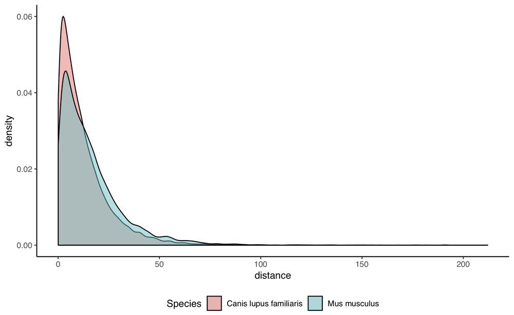
In this example, we compare the distribution of PAM distances (Point accepted mutations; 27) between orthologs of two species-pairs, namely human-dog and human-mouse. First, we request the required data:
mouse_id = getGenome(id='Mus musculus')$taxon_id
human_id = getGenome(id='Homo sapiens')$taxon_id
dog_id = getGenome(id='Canis lupus familiaris')$taxon_id

human_mouse <- getGenomePairs(genome_id1 = human_id,
    genome_id2 = mouse_id, rel_type = '1:1')

human_dog <- getGenomePairs(genome_id1 = human_id,
    genome_id2 = dog_id, rel_type = '1:1')
We can then bind the two resultant data frames and plot the results (Figure 3), as so:
human_mouse$Species <- 'Mus musculus'
human_dog$Species <- 'Canis lupus familiaris'

all_pairs <- rbind(human_mouse, human_dog)
all_pairs$Species <- as.factor(all_pairs$Species)

library(ggplot2)

g <- ggplot(all_pairs, aes(x = distance, fill = Species)) +
    geom_density(alpha = 0.5) +
    xlab('evolutionary distance [PAM]') +
    theme(legend.position = 'bottom', panel.grid.major =
    element_blank(), panel.grid.minor = element_blank(),
    panel.background = element_blank(), axis.line = element_line(colour
    = 'black'))
print(g)
The two-sample Kolmogorov-Smirnov test can be performed on the two distributions, using the command:
ks.test(human_dog$distance, human_mouse$distance)This returns p-value < 2.2e-16. The median distance between dog and human is shorter than that of mouse and human (8.8 vs. 11.8). This is consistent with previous observations that the rodent has a longer branch than humans and carnivores, in part due to their shorter generation time28.
Although the OMA database currently analyses over 2,100 genomes, many more have been sequenced, and the gap keeps on widening. It is nevertheless possible to use OMA to infer the function of custom protein sequences through a fast approximate search against all sequences in OMA4.
# Our mystery sequence is cystic fibrosis transmembrane conductance
# regulator in the Emperor penguin (UniProt ID: A0A087RGQ1_APTFO)
mysterySeq <-
'FFFLLRWTKPILRKGYRRRLELSDIYQIPSADSADNLSEKLEREWDRELATSKKKPKLINALRRCFFWKFM
FYGIILYLGEVTKSVQPLLLGRIIASYDPDNSDERSIAYYLAIGLCLLFLVRTLLIHPAIFGLHHIGMQMRI
AMFSLIYKKILKLSSRVLDKISTGQLVSLLSNNLNKFDEGLALAHFVWIAPLQVALLMGLLWDMLEASAFSG
LAFLIVLAFFQAWLGQRMMKYRNKRAGKINERLVITSEIIENIQSVKAYCWEDAMEKMIESIRETELKLTRK
AAYVRYFNSSAFFFSGFFVVFLAVLPYAVIKGIILRKIFTTISFCIVLRMTVTRQFPGSVQTWYDSIGAINK
IQDFLLKKEYKSLEYNLTTTGVELDKVTAFWDEGIGELFVKANQENNNSKAPSTDNNLFFSNFPLHASPVLQ
DINFKIEKGQLLAVSGSTGAGKTSLLMLIMGELEPSQGRLKHSGRISFSPQVSWIMPGTIKENIIFGVSYDE
YRYKSVIKACQLEEDISKFPDKDYTVLGDGGIILSGGQRARISLARAVYKDADLYLLDSPFGHLDIFTEKEI
FESCVCKLMANKTRILVTSKLEHLKIADKILILHEGSCYFYGTFSELQGQRPDFSSELMGFDSFDQFSAERR
NSILTETLRRFSIEGEGTGSRNEIKKQSFKQTSDFNDKRKNSIIINPLNASRKFSVVQRNGMQVNGIEDGHN
DPPERRFSLVPDLEQGDVGLLRSSMLNTDHILQGRRRQSVLNLMTGTSVNYGPNFSKKGSTTFRKMSMVPQT
NLSSEIDIYTRRLSRDSVLDITDEINEEDLKECFTDDAESMGTVTTWNTYFRYVTIHKNLIFVLILCVTVFL
VEVAASLAGLWFLKQTALKANTTQSENSTSDKPPVIVTVTSSYYIIYIYVGVADTLLAMGIFRGLPLVHTLI
TVSKTLHQKMVHAVLHAPMSTFNSWKAGGMLNRFSKDTAVLDDLLPLTVFDFIQLILIVIGAITVVSILQPY
IFLASVPVIAAFILLRAYFLHTSQQLKQLESEARSPIFTHLVTSLKGLWTLRAFGRQPYFETLFHKALNLHT
ANWFLYLSTLRWFQMRIEMIFVVFFVAVAFISIVTTGDGSGKVGIILTLAMNIMGTLQWAVNSSIDVDSLMR
SVGRIFKFIDMPTEEMKNIKPHKNNQFSDALVIENRHAKEEKNWPSGGQMTVKDLTAKYSEGGAAVLENISF
SISSGQRVGLLGRTGSGKSTLLFAFLRLLNTEGDIQIDGVSWSTVSVQQWRKAFGVIPQKVFIFSGTFRMNL
DPYGQWNDEEIWKVAEEVGLKSVIEQFPGQLDFVLVDGGCVLSHGHKQLMCLARSVLSKAKILLLDEPSAHL
DPVTSQVIRKTLKHAFANCTVILSEHRLEAMLECQRFLVIEDNKLRQYESIQKLLNEKSSFRQAISHADRLK
LLPVHHRNSSKRKPRPKITALQEETEEEVQETRL'
myAnnotations <- annotateSequence(mysterySeq)
This results in 54 GO annotations. By comparison, this sequence has merely 15 GO annotations in UniProt-GOA29 — all of which are also predicted by this method in OMA.
We go back to the lactotransferrin gene family from Example 2. We can use OmaDB in conjunction with the BgeeDB Bioconductor package30 to retrieve expression data from the Bgee database31 as follows.
BiocManager::install("BgeeDB")
library(BgeeDB)

# Bgee uses Ensembl gene IDs, obtainable using OmaDB’s cross-references.
trfl_xrefs <- getProtein(id='TRFL_HUMAN')$xref
trfl_ens_id <- subset(trfl_xrefs, source == 'Ensembl Gene')$xref
# The Ensembl gene IDs need to be without version suffix
trfl_ens_id <- strsplit(trfl_ens_id,'.',fixed=TRUE)[[1]][1]

my_stage <- 'UBERON:0034920' # Infant stage
bgee.expr <- Bgee$new(species='Homo_sapiens')
expr.data <- loadTopAnatData(bgee.expr, stage = my_stage)
gene.expr.tissue.ids <-
    unlist(expr.data$gene2anatomy[trfl_ens_id], use.names = F)
tissues <- expr.data$organ.names
print(tissues[tissues$ID %in% gene.expr.tissue.ids, ])
Among the tissues in which lactotransferrin is expressed according to Bgee (Table 2), we note the bone marrow and the palpebral conjunctiva (the eyelid inner surface). This is consistent with the aforementioned involvement of lactotransferrin in bone formation and anti-microbial activity.
| ID | Name |
|---|---|
| UBERON:0001812 | palpebral conjunctiva |
| UBERON:0000178 | blood |
| UBERON:0002371 | bone marrow |
| UBERON:0001154 | vermiform appendix |
| UBERON:0002084 | heart left ventricle |
Further tutorials on the OmaDB package can be found in the accompanying vignettes:
browseVignettes('OmaDB')
Orthology is used for various purposes, such as species tree inference, gene evolution dynamic, or protein function prediction. The retrieval of orthologs is thus typically just the starting point of a larger analysis. Therefore, this overhaul and expansion of the OMA programmatic interface will facilitate the incorporation of OMA data in such larger analyses.
Our R package will continue to be maintained in line with the biannual Bioconductor releases. Further work to improve the package includes improvement in performance. For example, the responses are currently fully loaded into an R object of choice which, depending on the response size, may create some time lag in the response. We will also continue to update the package and the API in sync with the OMA browser to incorporate new functionalities of OMA.
Likewise, we will also maintain and further develop the Python package. In particular, we will explore the possibility of further integration with the BioPython library32.
More generally, in OMA we will keep supporting the various ways of accessing the underlying data, including the interactive web browser and flat files in a variety of formats. The REST API is also complemented by a new SPARQL interface that enables highly specific queries, as well as federated queries over multiple resources4. However, the query language is more complex.
We very much welcome feedback and questions from the community. We also highly appreciate contributions to the code in the form of pull requests. Our preferred channel for support is the BioStar website33, where we monitor all posts with keyword “oma”.
Please note that this manuscript uses version 2.0 of the OmaDB R package, which is in the development version of Bioconductor (v.3.9). Until the release of Bioconductor v.3.9 in Spring 2019, there are two possible ways of installing it:
1) Install the development version of R (v.3.6) — required for Bioconductor v.3.9 — and install OmaDB using the command:
BiocManager::install('OmaDB', version = 'devel')
–or–
2) Install OmaDB 2.0 directly from the github repo using the devtools R package:
install.packages('devtools')
library(devtools)
install_github('dessimozlab/omadb')
REST API available from: https://omabrowser.org/api
Documentation available from: https://omabrowser.org/api/docs
R OmaDB package available from: http://bioconductor.org/packages/OmaDB/
Source code available from: https://github.com/DessimozLab/OmaDB/
Archived source code as at time of publication: http://doi.org/10.5281/zenodo.259508634
License: GPL-2
omadb Python package available from: https://pypi.org/project/omadb/
Source code available from: https://github.com/DessimozLab/pyomadb/
Archived source code as at time of publication: http://doi.org/10.5281/zenodo.253025035
License: GPL-3
We also provide a binder to reproduce in Python the analyses done in R. This is available from: https://mybinder.org/v2/gh/DessimozLab/pyomadb/master?filepath=examples%2Fpyomadb-examples.ipynb
| Views | Downloads | |
|---|---|---|
| F1000Research | - | - |
|
PubMed Central
Data from PMC are received and updated monthly.
|
- | - |
Provide sufficient details of any financial or non-financial competing interests to enable users to assess whether your comments might lead a reasonable person to question your impartiality. Consider the following examples, but note that this is not an exhaustive list:
Sign up for content alerts and receive a weekly or monthly email with all newly published articles
Already registered? Sign in
The email address should be the one you originally registered with F1000.
You registered with F1000 via Google, so we cannot reset your password.
To sign in, please click here.
If you still need help with your Google account password, please click here.
You registered with F1000 via Facebook, so we cannot reset your password.
To sign in, please click here.
If you still need help with your Facebook account password, please click here.
If your email address is registered with us, we will email you instructions to reset your password.
If you think you should have received this email but it has not arrived, please check your spam filters and/or contact for further assistance.
Comments on this article Comments (0)