Keywords
Structural Variant, Graph Genome, Human Genomics, Clinical Annotation, Quality Control, Codeathon
This article is included in the Hackathons collection.
Structural Variant, Graph Genome, Human Genomics, Clinical Annotation, Quality Control, Codeathon
Structural variants (SVs) are large-scale genomic alterations, frequently defined as greater than 50 bases (bp) in length, involving deletions, duplications, insertions, inversions and/or translocations, and can occur in combinations. SVs have been linked to multiple phenotypic differences between organisms, as well as within populations of the same species1,2. SVs are known to play roles in myriad diseases, including neurological (e.g. Parkinson, Huntington), Mendelian3, and other genomic alterations such as those seen in many cancers and constitutional diseases4–7. In contrast to single nucleotide variants (SNVs), involving substitution of a single nucleotide, SVs remain understudied due to their more complex nature1. Our understanding of these larger forms of genomic alterations is limited by the sequencing technology and computational methods available to analyze ever-increasing amounts of sequence or similar data. A special type of SV is copy number variant (CNV). These are unbalanced SVs that could either increase or decrease total DNA content through duplications and deletions, respectively. CNVs of high importance are associated with different physical diseases like obesity8,9, type 1 diabetes10, rheumatoid arthritis10, and neurological disorders such as autism11, schizophrenia12, Mendelian diseases and other genomic disorders. More general studies examine the relationship between copy number variation and a range of diseases13,14.
Recent studies report between 20,000 to 25,000 SVs per human genome1. Although the number of SVs per individual is smaller than that for SNVs, SVs account for more altered nucleotides per diploid genome15. Recently, there has been a prominent shift towards studying SVs at the population level. The most prominent and early example of this was the 1000 Genomes Project16, representing different ethnic groups. Other projects include National Institutes of Health (NIH)-sponsored programs such as the National Human Genome Research Institute (NHGRI)’s Centers for Common Disease Genomics (CCDG), and National Heart, Lung, and Blood Institute (NHLBI)’s Trans-Omics for Precision Medicine (TOPMed) program that includes ~155,000 participants sequenced. With data from newer, high-throughput sequencing platforms, investigators are able to capture the genetic variability at a genomic scale of SVs across more geographically and genetically distinct populations. The Icelandic project17 studied 1,817 Icelandic individuals, including 369 trios (mother+father+child). Accordingly, many tools exist to study SVs in cohorts (e.g. svtools18 and the StructURal Variant majorIty VOte (SURVIVOR)19).
Our understanding of genomic variability in humans is tied to the technologies used to study those genomes, typically involving DNA sequencing. Short-read (SR) DNA sequencing (resulting in reads usually less than 150 bp in length) has been the most common way to evaluate DNA samples directly, and RNA samples indirectly after cDNA conversion20,21. When short reads are mapped to reference genomes, they either map entirely or partially22. Partial mapping can be accomplished by locally aligning part of the read and dropping the rest. This is known as soft-clipping. However, short reads do not align well to large variants when there is a significant gap between the last anchored reference position of the read and position of the soft-clipped portion (e.g. a variant with repetitive sequences longer than the read itself)23. Therefore, the aligner may not produce a global alignment between the read and reference, either choosing not to map the entire read or leaving the soft-clipped portion unmapped1.
The linear reference genome (LRG), which is based on a linear coordinate system, is a common way to represent variability within a genome24,25. While this may be efficient for applications using one or few genomes, more complex applications using multiple LRGs do not scale well. For example, when mapping reads from RNA sequencing (RNA-seq) to a single genome, the use of an LRG requires a baseline amount of compute resources. However, if mapping to multiple linear reference genomes, the task scales roughly linearly, (increasing by a factor n, where n is the number of LRGs to which data can be mapped).
By contrast, graph genomes can explicitly encode many alternate paths. Variants can be represented in this data structure, and reads can then be mapped exactly to both a reference path and variant sequences. Graphs have been shown to reduce reference bias and improve read mappings to variants26–28. Variants can also be quickly genotyped from such structures. However, adding more variations can rapidly increase the complexity of the graph. In order to make the problem computationally tractable, one must carefully choose which genomic regions to include. Tools for working with graphs are still nascent, and there are few open-source graph implementations that enable mapping directly to SVs (e.g. vg27 and Paragraph28). Graphs are a non-linear alternative to represent genomes; different paths are presented in the graph data structure. Consequently, 1.) they can decrease reference bias and improve read mappings to variants26–28; and 2.) variants can be efficiently genotyped. Adding more genomes to the graph enhances it, but increases its complexity. To decrease complexity and make this problem computationally tractable, the added regions must be chosen carefully.
Regardless of how drastically human individuals may differ in features such as their physical characteristics and behaviors, the human genomes between any two people are actually relatively well-conserved across individuals. The completion of de novo individual genomes is costly, and population-scale comparisons impossible with current technology infrastructure. There are a small number of individuals represented in the reference human genome, while in comparison any given human individual has on average ~4 million single-nucleotide polymorphisms (SNPs) and ~2,500 CNVs16,29. Consequently, there is a burgeoning awareness that the current standard reference genome assemblies do not include available human variation data. Moreover, there is an urgent need for improved tools, which more precisely represent rare genotype(s) of individuals bearing haplotype(s) absent from the human genome30,31. This is particularly relevant for genomic variants leading to clinical phenotypes such as in Mendelian diseases and genomic disorders where rare and ultra-rare variants have a prominent role. A reliable and scalable solution to this comprises developing a more comprehensive reference genome data structure that represents variations that exist in a given population, such as a graph genome8. The variants in a given cohort’s genomic sequences are represented as independent walks along the graph, allowing it to represent the reference cohort.
Overall, the quality assessment, representation, and annotation of SVs across multiple disciplines (e.g. whole-genome sequencing (WGS) and metagenomic sequencing) remain challenging. Thus, our SV codeathon groups focused on seven topics, which led to development of seven new computational methods. These topics included: 1.) quality assessment of population-scale VCF files; 2.) metagenomic assembly quality assessment; 3.) CNV detection and identification of de novo SVs using long-reads; 4.) fast genome graph generation; 5.) SV annotation; 6.) graph making and graph-based read-mapping with GPUs; and 7.) CNV detection quality control. Here we describe our progress, giving details about our tools’ implementations and applications to foster continuous development beyond the current scope of the tools as they were at the end of this codeathon. All methods are open source licensed, and have been made available on GitHub (https://github.com/NCBI-Codeathons/).
Clouseau: rapid quality assessment of population-scale VCF files. As we progress from comparing SVs between a sample and its corresponding reference (capturing differences between a given sample and its reference genome) to large cohort genomic datasets (variants across multiple hundreds to thousands of samples), large variant call format (VCF) files are being generated. Generating these large VCF files often involves customized scripts or analysis methods leaving the possibility of human or other runtime errors. For example, undetected errors such as incomplete files or artificially missing data might be mistaken for real biological phenomena (deletions/truncations). Leaving these unchecked may lead to erroneous conclusions. We developed Clouseau to address these challenges. Clouseau is a command line tool allowing users to rapidly validate VCF file formatting, generate multiple QC statistics, providing rapid QC insights from the input VCF file.
MasQ: Metagenomic assemblies-focused Quality assessment. While metagenomic assemblies have significantly improved since the early days of the Human Microbiome Project (HMP), intragenomic and intergenomic repetitive sequences remain as confounders. Individual reads spanning microbial strains (either via long-read technology or by generating synthetic long-reads) may be pieced together to resolve variation within a given microbial community. However, this process is imperfect. A major concern is that detected structural variants could actually result from misassembled genomic data instead of actual strain-specific variation. The goal of this project is to identify errors in any metagenomic assembly based on both short and long read mapping, in the hope of eliminating some of the uncertainty and error in metagenomic studies. Examples of errors to detect include falsely called (false positive) inversions, chimeras (translocation), INDELs (less than 50 bases long), and replacements (large substitutions). We created a containerized quality control pipeline called MasQ to locate, classify, and rectify errors in metagenomic assemblies. Out of concern for the integrity of current and future metagenomic studies from short-read and long-read genome sequencing data, we found that the quality control of metagenomic assemblies could be substantially improved by using a combination of sequence alignment tools and VCF file outputs from SV callers such as Sniffles v1.0.832 and Manta v1.5.033. The resulting SV call sets are subsequently compared and merged using packages like Truvari v0.1.2018.08.1 and SURVIVOR19. The current version of MasQ neatly packages this workflow and integrates it with novel correction and validation steps to fix any erroneous contigs found.
DeNovoSV: CNV detection and identification of de novo SV events using long reads. We developed a pipeline to identify de novo structural variants (SVs) from long-read (LR) sequencing data collected from trios (probands + parents). As described below, in a pilot study, we analyzed data from an individual who carries multiple de novo CNVs, initially identified by array-based comparative genomic hybridization (aCGH). Prior to this work, we lacked an integrated bioinformatics pipeline to identify high-confidence, de novo structural variants called from LR DNA sequencing (e.g., Oxford Nanopore Technology - ONT). Accordingly, to select further SV calls for orthogonal validation, we merged de novo LR SV calls with de novo SV calls independently identified by short-read (SR) DNA sequencing (i.e. PCR-free paired-end Illumina DNA sequencing, 150 paired-end reads, 40x depth of coverage) in this trio. DeNovoSV facilitates identification and prioritization of high-quality de novo SV calls that can be further validated by using targeted orthogonal methodologies such as Sanger sequencing or droplet digital PCR (ddPCR).
SWIGG (SWIft Genomes in a Graph): fast genome graph generation. There is a growing consensus across genomics that linear genome representation is suboptimal for representing variants across populations. While graph genomes have been steadily gaining popularity, many challenges remain (complexity, visualization, etc.). In this project, we developed a heuristic approach that quickly generates graphs and represents genomes in an efficient and succinct way. We created a simple algorithm and tool to build a graphical model that captures variability in the genomes at multiple scales. Moreover, there are regions across the human genome that are conserved among species while bearing modest amounts of variability that are suitable for understanding relationships of genome structure among individuals and/or organisms. We used a k-mer approach to create a sparse representation of such regions (anchors) at a large scale so as to allow visualizing the entire genome easily. These "anchored" graphs can then be further iteratively improved to include local sequence differences, and in turn, to help with genotyping existing variants and identifying new variants in new genomes.
ASAP (Automated Structural Variation Annotation Pipeline). ASAP is an automated and robust pipeline to annotate structural variations. The pipeline integrates annotations including allele frequency, colocated gene, functional features, domains, regulatory elements, and transcription levels. To facilitate further development, we took a pseudo-multistage build approach. Specifically, during stage one, we pull the main program, AnnotSV v2.234 from its remote source, as we expect this step to change relatively infrequently and the program itself is large. In stage two, based on the previously-built base image, we pull in its dependencies including BEDtools v2.29.035 and build the docker. The workflow is as follows: 1.) User provides a VCF containing SV as input into AnnotSV 2.) AnnotSV annotates the variations and outputs a tab-delimited file 3.) the R script “postprocess.R” is used to process the TSV file generated by AnnotSV and extracts essential annotations like ranking score. AnnotSV has many default annotation sources (https://lbgi.fr/AnnotSV/), and can also accept user-provided annotations as input. The output of this pipeline used the default annotation.
Super-minityper: graph making and graph-based read-mapping with GPUs in the cloud. We present a set of cloud-based workflows, composed mostly of preexisting and optimized tools, to 1.) construct graphs containing structural variants and 2.) map reads to these graphs. Our workflows allow users to make arbitrary SV calls, construct a graph, and map reads to these graphs. This workflow prioritizes ease-of-use and speed, accepting common input formats and returning results in minutes on commodity cloud virtual machines. Our approach is an example of what can be done now, and is generalizable to newer graph tools.
ScanCNV. Many current medical genomic studies still rely on CNV calling to identify de novo events that could have led to a certain disease phenotype. Nevertheless, a common problem for CNV detection is a high rate of false positives36 due to multiple biases in leading short-read sequencing technologies (e.g. GC bias, repetitiveness and general unevenness of the sequence data). To identify false positives and thus improve the reliability of CNV calling pipelines, we designed ScanCNV, which includes multiple QC steps. These QC steps currently include FASTQC v0.11.9, XYAlign v1.1.637, and Plink v2.038 where all the information is currently assembled and vetted within ScanCNV. Future work is still required to automate the process and fully leverage the obtained QC results.
All methods were tested on DNA-Nexus instances azure:mem1_ssd1_x, 4, cores, 8G ram or azure:mem1_ssd1_x16, 16 cores, 32G ram.
Clouseau. Clouseau requires python 3.5 or above. Users supply optional parameters such as the expected maximum distance between variations to identify missing entries. Importantly, the input VCF file needs to be sorted by coordinates. The Clouseau pipeline reads in a VCF file and performs a sample-level basic statistic carried out to ensure that the VCF file is complete and was not truncated during the VCF generation. Next, the VCF is parsed and sample-level QC is carried out. This consists of checking the number of samples in the VCF, the number of chromosomes, the names of all chromosomes/contigs, the distribution and number of variants (single nucleotide variants, insertions, deletions, structural variants) in each chromosome/contig for all samples, and the coordinates for the start and end of each variant for each chromosome and sample. Clouseau further tries to identify missing entries based on long stretches of no variations, which might represent file errors (as occur in incomplete files) or real biological phenomena (as in deletion/truncation). The full workflow is shown in Figure 1.
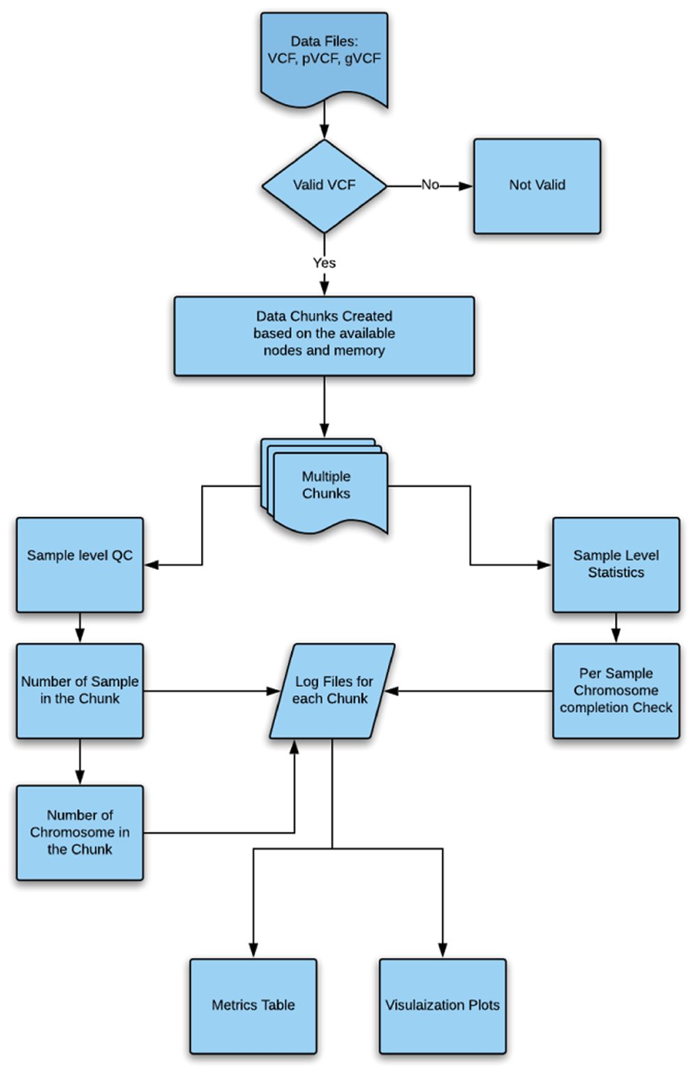
Clouseau starts with a VCF/pVCF/gVCF (variant call format) file that is assessed to ensure the completeness of the previous run. Furthermore, Clouseau assesses the overall statistics to give insights into the per sample quality control (QC). VCF, variant call format. pVCF, project variant call format. gVCF, genome variant call format. QC, quality control.
MasQ. The MasQ pipeline comprises four stages for metagenomic study quality control and validation: assembly, classification, correction, and validation. Our pipeline takes read files in FASTQ format as input, and classifies possible assembly errors as inversions, INDELs, substitutions, chimeras, or N/A, and then compares them with the make-up of the original assembly.
The purpose of the assembly stage is to do basic quality control on the sequencing data, generate a mock assembly from alignments of the read data, and generate VCF files informing about identified errors. Short-reads are pre-processed and visually assessed for quality, using FastQC. Then, all the reads are aligned to the MegaHIT assembly using BWA-MEM v0.7.439. The alignment results are processed through Manta v1.5.033, a structural variant caller, to produce a VCF file containing the detected errors. Optionally, if long reads are also available for the same sequencing sample, they are passed through a similar pipeline. The long reads are inspected for quality using NanoporeQC. Minimap2 v2.840 is used to align the long reads instead of BWA, then the long-read alignments are provided to Sniffles v1.0.832 to call SVs, condensing this information into a VCF file.
In the classification stage, VCF files for the short and long reads are compared to each other using Truvari and a merged VCF file is generated with SV data. Short-read and long-read data each present their own sets of challenges while building metagenomic assemblies, so comparison of the Truvari results from short and long sequencing reads of the same samples decreases false positive results.
The correction stage takes the regions of assembly error ascertained from the classification stage and performs the necessary changes to make a more accurate metagenomic assembly. From here, the validation stage uses sequence aligners such as Minimap2 and BWA to compare the edited assembly to the original inputs, looking to confirm an increase in the percentage of mapped reads in the corrected assembly, which would show the success of the pipeline in locating and correcting assembly errors.
MasQ is implemented using Docker and is freely available on DockerHub. MasQ can also be run online using DNAnexus. All relevant parameters, as well as python scripts for the correction and validation steps, can be found on the GitHub repository. The MasQ pipeline is shown below in Figure 2.
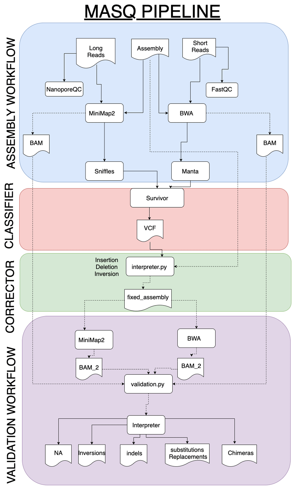
Over multiple steps MasQ utilizes the short and long reads available to assess the quality of the before obtained metagenomic assembly.
DeNovoSV. DeNovoSV takes input VCF files produced by long-read SV callers such as Sniffles v1.0.1132 and short-read SV callers such as Lumpy v0.2.1341, Delly v0.8.242, and Manta v1.6.033. We developed a custom shell script to remove calls that genotyped as a homozygous reference (GT=0/0), with read support less than 5 and aligned to haplotype chromosome, unplaced or unlocalized contigs (GL, KI, etc). Second, the filtered outputs are combined and compared by the pipeline using SURVIVOR v1.0.619 merge allowing a maximum distance of 1000 bp measured pairwise from the start and end breakpoints of each SV, respectively; SVs classified as the same type; and SVs larger than 30 bp. Lastly, CNV calls are performed independently, using ONT data calculated on the resulting alignments using mosdepth v0.2.343 with the following parameter set “-F 3588 -Q 1”. This calculates the bp coverage in 100 kb bins and includes only primary and supplemental alignments. Normalization of the coverage signal is performed based on a custom script, which generates bedgraph data as output. Each individual bedgraph file pertaining to proband and parents is processed by dividing the 100 bp bins scores by the median of the coverage windows. Using this normalization, the majority of the genome shows a score of 1 (ie. similar coverage between the samples) while a CNV on the proband results in a score of 2 for a duplication. We load these files into JBrowse44 with the multibigwig plugin for visualization, and to facilitate downstream analyses of the putative CNV calls. The resulting output is a list of high-confidence de novo SVs. The overall workflow of DeNovoSV is shown in Figure 3.
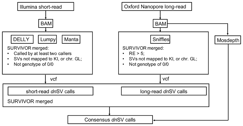
The schematic shows the required inputs and final outputs, along with intermediate steps. DeNovoSv starts with already aligned reads (BAM) from long reads and short reads to filter candidate SVs based on a trio to identify de novo SVs in the proband.
SWIGG. The SWIGG (SWIft Graph in a Genome) pipeline can take multiple FASTA sequences as input and outputs a graph that would be a sparse representation for a multiple sequence alignment which can be visualized for larger scale differences. First, the input FASTA sequence is processed to identify appropriate k-mers. Appropriate k-mers are those that are not repetitive within and across all FASTA sequences. The thresholds for appropriate k-mers can be modified using the script arguments. K-mers are then sorted based on their positions and collapsed into a node-edge list. This node-edge list can be visualized using a graph visualizer such as Gephi.
Our motivation to implement SWIGG (Figure 4) is that the human genome essentially contains two types of regions, those that are quite stable, and those that are hypervariable45,46. For the stable regions, short reads can be either hashed as exact matches to these relatively static regions, or mapped with very small bubbles. Nevertheless, stable regions are interspersed by variable and hypervariable regions (e.g. Kir, MSC). We used k-mers to provide a backbone for these complex regions. Likewise, we have also looked at those regions that are very unstable for mapping in the reference genome to extrapolate to graphs. We used 64 of such regions located on human chromosome 6. They are graphically depicted using the NCBI Genome Data Viewer47 in Figure 5. SWIGG is implemented in python 3 and publicly available both on GitHub.
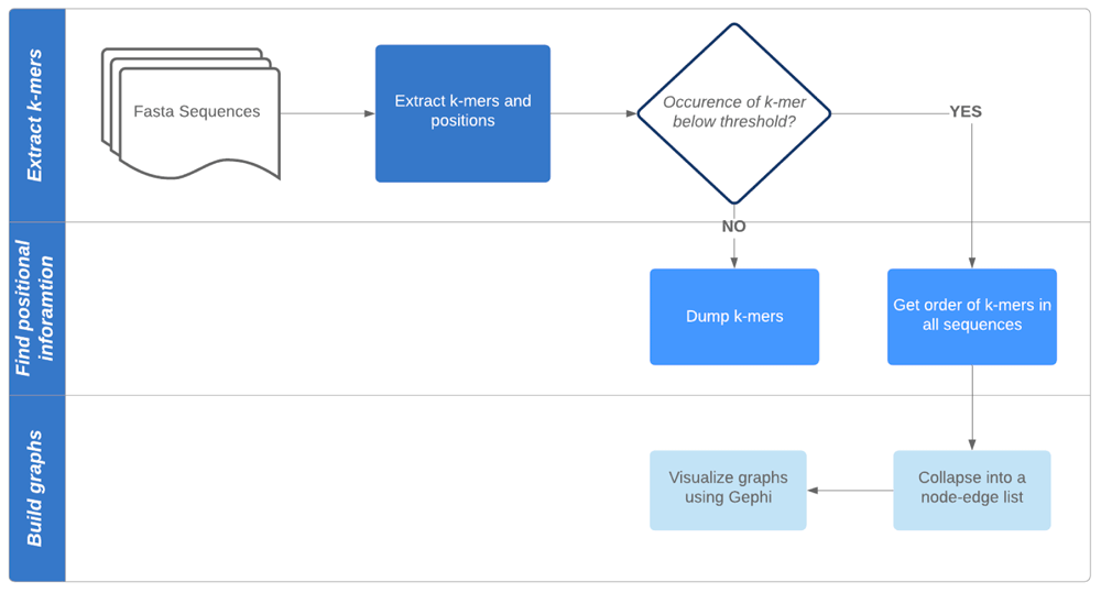
ASAP. The user inputs an SV VCF file(s) produced from any SV caller, and the SV file is then ranked and annotated using AnnotSV and produces a tab-delimited file which will be processed using contemporary versions of R. The complete pipeline can be executed automatically as a single WDL script on GitHub. Below is the workflow Figure 6.
Before proceeding with SV analysis, the user needs to have insight into the SV file to avoid issues with downstream analyses. Clouseau facilitates this best-practice quality control check by analyzing an input SV file and providing detailed information about its content. Clouseau takes as input an SV VCF file, and returns the number of samples in the file, chromosomes analyzed, distribution of SVs in all samples, and detailed information about each sample in the file. The output is a list of files for all the samples and each sample in the input file. Clouseau was benchmarked using the SV file from the 1000 Genomes Project16. The data set consists of 2,505 samples and consumed 1 minute (wall clock time) to analyze 10,000 variant lines, Figure 7 shows an example of the output results per sample.
MasQ uses short- and long-read sequencing data as input. It outputs VCF files with the locations of structural variants, as well as a classification of assembly errors. Among the two existing methods of assembly validation, reference-based or de novo assembled, we chose to develop a de novo validation pipeline, and benchmarked it using two widely-used datasets, Zymo Microbial Community Standards48 and Shakya49. The Zymo dataset consisted of both Illumina pair-ended short reads and Oxford Nanopore long reads, while the Shakya dataset was made up of pair-ended short reads. The current version of MasQ is publicly available as a Docker container that combines existing tools for assembly, creation and comparison. It includes a Python classifier and correction to identify and fix assembly errors, and is open source on GitHub.
For the Shakya49 data, metaSPAdes50 assembly, metaQUAST51 reports that there are 328 misassemblies and the total misassembled contigs length is 12,555,565 base pairs. For Shakya, MEGAHIT52 assembly, metaQUAST reports that there are 673 misassemblies and the total misassembled contigs length is 20,244,280 base pairs. For both of the finished assemblies, metaQUAST reports more than hundreds of misassemblies and the total length is more than tens of million base pairs. Also, on the Shakya dataset, according to metaQUAST, the performance of metaSPAdes is slightly better than that of the MEGAHIT. For the MasQ result of both assemblies, both Manta and Sniffles call hundreds of mis-assemblies in two assemblies, which are about the same size of the result outputted by metaQUAST. From the long-read perspective, Sniffles calls less insertions and duplications on the metaSPAdes assembly. Even though metaSPAdes required significantly more time to finish assembling, the extension of edges through repetitive regions and careful decision to remove low coverage edges contributed to a lower insertion and duplication rate.
In a prototype trial of DeNovoSV, we investigated available genomics data obtained from a trio of samples (i.e. father, mother and proband), with a particular focus on identification of de novo SVs in the proband. Available data included ONT long-read sequences, Illumina short-read WGS from the trio and aCGH. Data from the latter were used as a positive control for known de novo CNVs for the purpose of developing this pipeline. Working with ONT long-read sequence data, we used the NGMLR32 aligner to map the data against the human genome reference assembly (hg38). Sniffles32 used BAM files from the previous step to identify candidate de novo SVs. Read depths of SVs were calculated using mosdepth43. Sniffles outputs were used as source dataset for VCF files which were filtered using our DeNovoSV custom script to remove SVs for which supporting reads were limited in number (RE < 5); homozygous reference SVs; SV branching from autosomes to decoy; and contigs identified with GL numbers, which represent unlocalized contigs. De novo SVs in the child were defined by merging and comparing with parents in the trio using SURVIVOR19. After filtering for de novo SVs in the child using the DeNovoSV pipeline, we compared these de novo SVs and CNV candidates with results extracted from CGH array data.
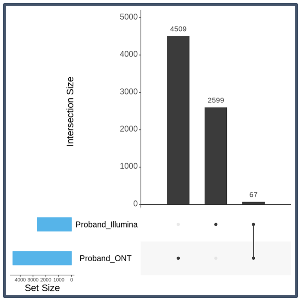
We used the DeNovoSV pipeline to prioritize high-confidence, de novo SVs called from long-read (LR) technology. Starting with about 3 million SV calls identified by Sniffles for each individual, the de novo LR pipeline detected 4,509 high-quality SV calls. We further enriched for potentially true-positive calls by merging the long-read calls with SVs calls independently identified with short-read sequencing in this trio (N = 2599 high-quality SV calls). After merging the calls from short-read sequencing to filter for consensus calls, we obtained a list of 67 high-quality SV calls (Figure 8 and Figure 9).
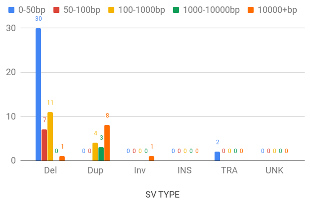
Del: deletion; Dup: duplication; Inv: inversion; INS: insertion; TRA: translocation; UNK: unknown.
Eight de novo duplications in the proband were detected using normalized read depth coverage data from mosdepth and visualized in JBrowse (Figure 10).
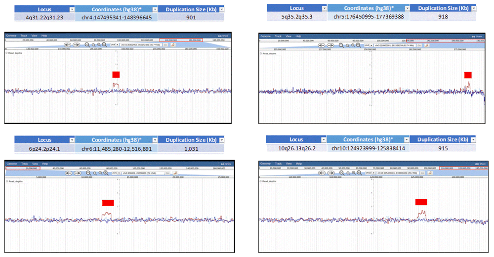
JBrowse screenshots displaying normalized Oxford Nanopore read coverage for four out of eight de novo duplications spanning 900 kb to 1 Mb genomic segments from Chromosomes 4, 5, 6 and 10. Parent 1 is represented in a blue line, parent 2 in a light blue line and proband in a dark red line. Red rectangles denote duplications.
In SWIGG we created a simple algorithm and tool to build genome graphs, which is suitable for understanding relationships of genome structure among individuals and/or organisms. Our approach captured variations in a hierarchical way. The idea was to create a sparse representation of large-scale differences (anchors) so as to allow visualizing the entire genome in a succinct way. These "anchored" graphs can then be further iteratively improved to include local sequence differences, and in turn, facilitate genotyping existing variants and identifying new variants in new genomes. We tested SWIGG by creating a graph of the human MHC region (4.5Mb in size) Figure 11 using 128-mers in less than three minutes on seven alternative haplotypes. To evaluate our approach at a smaller scale, we tried building a graph for 10 HIV viral genome (each ~10kb) using 10-mers (see SWIGG Github repository).
ASAP was benchmarked using 53 non-diseased tissue sites across nearly 1000 individuals. GTEx RNA-seq data (retrieved from RNA-seq gene read counts GCT file https://gtexportal.org/home/datasets) and GTEx Metadata (manually curated from https://www.ebi.ac.uk/arrayexpress/files/E-MTAB-5214/E-MTAB-5214.sdrf.txt) from NA12878 Germline Whole Genome were used. V2 Chromium Genome dataset by Long Ranger 2.2.1 downloaded WGS v2 deletions VCF file from https://support.10xgenomics.com/genome-exome/datasets/2.2.1/NA12878_WGS_v2. Messenger RNA features were extracted from NCBI latest RefSeq Annotation53 on GRCh38 using instructions provided here https://www.ncbi.nlm.nih.gov/refseq/functionalelements/. The workflow for running benchmarking and results are shown in Figure 12 below.
The current version of Clouseau sought to validate VCF integrity and to provide informative statistics. Clouseau can read an SV file and return relevant reports. A next step would be to implement modules to accept SNVs, more than one file as an input, visualize the statistics results using publicly available modules, and reimplement the tool to guarantee better performance.
MasQ currently provides a smooth, convenient workflow to locate genome assembly errors and a solid foundation for a machine learning model to classify assembly errors. In the future, MasQ would benefit from further testing with simulated data, larger datasets, and manual annotation of training data for a more sophisticated classifier. We intend to treat this problem as a multiclass text classification problem, which could be successfully handled using an RNN, LSTM, SVM, or HAN framework (Figure 13). Additionally, the outputs from the classification model must be visualized with histograms of the assembly error types, as well as with visual indications of where the errors are located within the assembly. The assembly errors could possibly be organized so that each type of error could be queried within the given assembly and made easily accessible to users.
In a pilot study to analyze de novo SVs identified in a proband from a genetic trio, we evaluated capabilities of DeNovoSV to confirm those SVs and potentially to discover additional SVs. Using the DenovoSV pipeline with parameters described in Figure 3, all eight genome-wide chromosomal segments with known de novo duplications identified by aCGH in the proband were also identified by short- and long-reads. In addition, 59 additional potential de novo SVs were identified, which need further validation. Independently, the read depth information generated by mosdepth using LR data from ONT also successfully identified all eight genomic duplications, suggesting that analysis of LR data alone can be valuable for de novo CNV detection.
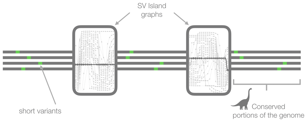
Once simple and variable regions are solved for graphs, including those with many structural variants and those with complex regions across a number of populations and diseases, then we will be able to phase new genomes automatically. Thus, we will be able to observe traversals of previously unmanageable paths through graphs made from both long and short read data as shown in Figure 14.
Now that we are developing tools for generating genome graphs quickly and efficiently, it is desirable to find optimal parameters (e.g. size of k-mer and occurrence of a k-mer) to determine whether a given graph should be retained or not. This remains challenging because there is no simple way to evaluate genome graphs. Numbers of nodes and edges can be starting points. Comprehensive investigations of potential factors are needed, such as determining to what extent known features are recapitulated in the graphs.
Clouseau - SV data from 2,505 samples from the 1000 Genomes Project (http://ftp.1000genomes.ebi.ac.uk/vol1/ftp/release/20130502/).
MasQ - Zymobiomics Microbial Community Standards Assemblies (10 genomes; 5 gram positive, 3 gram negative, 2 yeast). Each has a known reference. Synthetic bacteria included: Bacillus subtilis, Cryptococcus neoformans, Enterococcus faecalis, Escherichia coli, Lactobacillus fermentum, Listeria monocytogenes, Pseudomonas aeruginosa, Saccharomyces cerevisiae, Salmonella enterica, Staphylococcus aureus. Illumina pair-ended short reads from IMMSA dataset (ftp://ftp-private.ncbi.nlm.nih.gov/nist-immsa/IMMSA/). Shakya Assembly (assembled using MegaHIT and MetaSPAdes) - Each has a known reference. Synthetic bacteria included: Acidobacterium capsulatum, Aciduliprofundum boonei, Akkermansia muciniphila, Archaeoglobus fulgidus, Bacteroides thetaiotaomicron, Bacteroides vulgatus, Bordetella bronchiseptica, Burkholderia xenovorans LB400, Caldicellulosiruptor bescii, Caldicellulosiruptor saccharolyticus, Chlorobium limicola, Chlorobium phaeobacteroides, Chlorobium phaeovibriodes, Chlorobium tepidum, Chloroflexus aurantiacus, Clostridium thermocellum, Deinococcus radiodurans, Desulfovibrio piger, Desulfovibrio vulgaris, Dictyoglomus turgidum, Enterococcus faecalis, Fusobacterium nucleatum, Gemmatimonas aurantiacus, Geobacter sulfurreducens, Haloferax volcanii, Herpetosiphon aurantiacus, Hydrogenobaculum, Ignicoccus hospitalis, Leptothrix cholodnii, Methanocaldococcus jannaschii, Methanococcus maripaludis C5, Methanococcus maripaludis S2, Methanopyrus kandleri, Methanosarcina acetivorans C2A, Nanoarchaeum equitans, Nitrosomonas europaea, Nostoc sp. PCC 7120, Pelodictyon phaeoclatharatiforme, Persephonella marina EX-H1, Porphyromonas gingivalis, Pyrobaculum aerophilum IM2, Pyrobaculum arsenaticum, Pyrobaculum calidifontis, Pyrococcus furiosus, Pyrococcus horikoshii, Rhodopirellula baltica, Ruegeria pomeroyi, Salinispora arenicola, Salinispora tropica, Shewanella baltica OS185, Shewanella baltica OS223, Sulfitobacter sp.EE-36, Sulfitobacter sp.NAS-14.1, Sulfolobus tokodaii, Sulfurihydrogenibium sp.YO3AOP1, Sulfurihydrogenibium yellowstonense, Thermoanaerobacter pseudethanolicus, Thermotoga neapolitana DSM 4359, Thermotoga petrophila RKU-1, Thermotoga sp.RQ2, Thermus thermophilus HB8, Treponema denticola, Zymomonas mobilis. From Illumina pair-ended short reads. Number of sequences: 54814748. Read length: 101 bp.
DeNovoSV - For the development of the pipeline we used in-house control data from patients.
SWIGG - For data to construct the graph, we used the alternative sequences of the MHC region given in the latest reference Human Genome (HGR38). These were downloaded using NCBI accession numbers GL000250, GL000251, GL000253, GL000254, GL000255 and GL000256. HIV sequences were obtained from Los Alamos National Laboratories54, [with specific accession numbers] Human immunodeficiency virus type 1 (HXB2), complete genome; HIV1/HTLV-III/LAV reference genome [K03455], HIV-1 isolate 2106 from Democratic Republic of the Congo, complete genome [MH705158], HIV-1 isolate 50 from Democratic Republic of the Congo, complete genome [MH705161], HIV-1 isolate 70641 from Democratic Republic of the Congo, complete genome [MH705151], HIV-1 isolate P4039 from Democratic Republic of the Congo, complete genome [MH705157], HIV-1 isolate PBS6126 from Democratic Republic of the Congo, complete genome [MH705153], HIV-1 isolate PBS888 from Democratic Republic of the Congo, complete genome [MH705133], HIV-1 isolate HIV/CH/BID-V3538/2003 from Switzerland, partial genome [JQ403028], Human immunodeficiency virus 1 proviral env gene for envelope protein, isolate 98CM.MP1014 [AM279354], HIV-1 isolate 09NG010499 from Nigeria gag protein (gag) gene, complete cds; pol protein (pol) gene, partial cds; and vif protein (vif), vpr protein (vpr), tat protein (tat), rev protein (rev), vpu protein (vpu), envelope glycoprotein (env), and nef protein (nef) genes, complete cds. [KX389622].
ASAP - Data sources and Data Description: 53 non-diseased tissue sites across nearly 1000 individuals: GTEx RNASeq Data: Downloaded RNA-Seq gene read counts GCT file from https://gtexportal.org/home/datasets. GTEx Metadata: manually curated from https://www.ebi.ac.uk/arrayexpress/files/E-MTAB-5214/E-MTAB-5214.sdrf.txt from NA12878 Germline Whole Genome v2 Chromium Genome v2 Dataset by Long Ranger 2.2.1: Downloaded WGS v2 dels VCF file from from https://support.10xgenomics.com/genome-exome/datasets/2.2.1/NA12878_WGS_v2. RefSeq Features: mRNA features are extracted from NCBI latest RefSeq Annotation on GRCh38 using instructions provided here: https://www.ncbi.nlm.nih.gov/refseq/functionalelements/.
ScanCNV - Simulated CNV 6 samples (males and females) FASTQ data (truth set: “In silico CNVs - Sheet1.csv”), and 1000 Genomes 10 random samples (males and females) mapped data (in file names) in GitHub repository (see below).
Clouseau is available from GitHub: https://github.com/NCBI-Codeathons/Clouseau.
Archived source code at time of publication: https://doi.org/10.5281/zenodo.395042155
License: MIT
MasQ is freely available from GitHub: https://github.com/NCBI-Codeathons/MASQ.
Archived source code at time of publication: https://doi.org/10.5281/zenodo.395044156
License: MIT
DeNovoSV is freely available from GitHub: https://github.com/NCBI-Codeathons/DeNovoSV.
Archived source code at time of publication: https://doi.org/10.5281/zenodo.395043957
License: MIT
SWIGG is freely available from GitHub: https://github.com/NCBI-Codeathons/SWIGG.git.
DockerHub: ncbicodeathons/swigg.
Archived source code at time of publication: https://doi.org/10.5281/zenodo.395042558
License: MIT
ASAP is freely available from GitHub: https://github.com/NCBI-Codeathons/ASAP.
Archived source code at time of publication: https://doi.org/10.5281/zenodo.395044459
License: MIT
Super-minityper is freely available from GitHub: https://github.com/NCBI-Codeathons/super-minityper.
Archived source code at time of publication: https://doi.org/10.5281/zenodo.395043560
License: MIT
ScanCNV is freely available from GitHub: https://github.com/NCBI-Codeathons/SCANCNV.
Archived source code at time of publication: https://doi.org/10.5281/zenodo.397728361
License: MIT
We would like to thank the administrative staff of the Human Genome Sequencing Center at Baylor College of Medicine (especially Meagan Elizaheth Sam and Chelette Darlene Gaskin) who helped to organize and run the event. We thank DNAnexus Inc. for sponsoring cloud computing resources. We thank Drs. Pengfei Liu and James R. Lupski for generously providing data from their Multiple CNVs project for the DenovoSV pipeline development and Oxford Nanopore Technology team for helping with data generation and data analysis. We thank Dr. Nick Matinyan for helpful suggestions during manuscript review.
| Views | Downloads | |
|---|---|---|
| F1000Research | - | - |
|
PubMed Central
Data from PMC are received and updated monthly.
|
- | - |
Is the rationale for developing the new software tool clearly explained?
Yes
Is the description of the software tool technically sound?
Yes
Are sufficient details of the code, methods and analysis (if applicable) provided to allow replication of the software development and its use by others?
Yes
Is sufficient information provided to allow interpretation of the expected output datasets and any results generated using the tool?
Yes
Are the conclusions about the tool and its performance adequately supported by the findings presented in the article?
Yes
Competing Interests: No competing interests were disclosed.
Reviewer Expertise: bioinformatics, genomics, e-Health
Is the rationale for developing the new software tool clearly explained?
Yes
Is the description of the software tool technically sound?
Partly
Are sufficient details of the code, methods and analysis (if applicable) provided to allow replication of the software development and its use by others?
Partly
Is sufficient information provided to allow interpretation of the expected output datasets and any results generated using the tool?
Partly
Are the conclusions about the tool and its performance adequately supported by the findings presented in the article?
Yes
Competing Interests: No competing interests were disclosed.
Reviewer Expertise: Bioinformatics, Software development
Alongside their report, reviewers assign a status to the article:
| Invited Reviewers | ||
|---|---|---|
| 1 | 2 | |
|
Version 1 16 Sep 20 |
read | read |
Provide sufficient details of any financial or non-financial competing interests to enable users to assess whether your comments might lead a reasonable person to question your impartiality. Consider the following examples, but note that this is not an exhaustive list:
Sign up for content alerts and receive a weekly or monthly email with all newly published articles
Already registered? Sign in
The email address should be the one you originally registered with F1000.
You registered with F1000 via Google, so we cannot reset your password.
To sign in, please click here.
If you still need help with your Google account password, please click here.
You registered with F1000 via Facebook, so we cannot reset your password.
To sign in, please click here.
If you still need help with your Facebook account password, please click here.
If your email address is registered with us, we will email you instructions to reset your password.
If you think you should have received this email but it has not arrived, please check your spam filters and/or contact for further assistance.
Comments on this article Comments (0)