periodicDNA: an R/Bioconductor package to investigate k-mer periodicity in DNA

Jacques Serizay; Julie Ahringer

doi:10.12688/f1000research.51143.1

Home Browse periodicDNA: an R/Bioconductor package to investigate k-mer periodicity...

ALL Metrics

-

Views

-

Downloads

Get PDF

Get XML

Export

▬

✚

Software Tool Article

periodicDNA: an R/Bioconductor package to investigate k-mer periodicity in DNA

[version 1; peer review: 1 approved, 3 approved with reservations]

Jacques Serizay ¹, Julie Ahringer¹

PUBLISHED 24 Feb 2021

Author details Author details

¹ The Gurdon Institute and Department of Genetics, University of Cambridge, Cambridge, CB2 1QN, UK

Jacques Serizay
Roles: Conceptualization, Data Curation, Formal Analysis, Investigation, Methodology, Software, Validation, Visualization, Writing – Original Draft Preparation, Writing – Review & Editing

Julie Ahringer
Roles: Conceptualization, Funding Acquisition, Supervision, Writing – Original Draft Preparation, Writing – Review & Editing

OPEN PEER REVIEW

REVIEWER STATUS

This article is included in the Bioinformatics gateway.

This article is included in the Cell & Molecular Biology gateway.

This article is included in the RPackage gateway.

This article is included in the Bioconductor gateway.

Abstract

Periodic occurrences of oligonucleotide sequences can impact the physical properties of DNA. For example, DNA bendability is modulated by 10-bp periodic occurrences of WW (W = A/T) dinucleotides. We present periodicDNA, an R package to identify k-mer periodicity and generate continuous tracks of k-mer periodicity over genomic loci of interest, such as regulatory elements. periodicDNA will facilitate investigation and improve understanding of how periodic DNA sequence features impact function.

Keywords

DNA periodicity, gene regulation, promoter

Corresponding authors: Jacques Serizay, Julie Ahringer

Competing interests: No competing interests were disclosed.

Grant information: The work was supported by a Wellcome Trust Senior Research Fellowship to J.A. (101863) and a Medical Research Council DTP studentship to J.S..
The funders had no role in study design, data collection and analysis, decision to publish, or preparation of the manuscript.

Copyright: © 2021 Serizay J and Ahringer J. This is an open access article distributed under the terms of the Creative Commons Attribution License, which permits unrestricted use, distribution, and reproduction in any medium, provided the original work is properly cited.

How to cite: Serizay J and Ahringer J. periodicDNA: an R/Bioconductor package to investigate k-mer periodicity in DNA [version 1; peer review: 1 approved, 3 approved with reservations]. F1000Research 2021, 10:141 (https://doi.org/10.12688/f1000research.51143.1) First published: 24 Feb 2021, 10:141 (https://doi.org/10.12688/f1000research.51143.1) Latest published: 24 Feb 2021, 10:141 (https://doi.org/10.12688/f1000research.51143.1)

Introduction

Short DNA sequence motifs provide key information for interpreting the instructions in DNA, for example by providing binding sites for proteins or altering the structure of the double-helix. A less studied but important feature of DNA sequence motifs is their periodicity^1–4. Two famous examples are the universal 3bp periodic (RNY)_n pattern (R = A or G, Y = C or U, N = any base) in exons⁵ and 10-bp periodic k-mers in nucleosome positioning (reviewed in 6 and 7). However, despite the wealth of software focusing on motif discovery and analysis, no tool provides an easy way to quantify the periodicity of a given motif, i.e. the extent to which a given motif is repeated at a regular interval in specific sequences. For instance, HeliCis and SpaMo identify conserved distances between two motifs in sequences of interest, but they do not assess larger scale periodic occurrences of motifs^8,9.

Here we present periodicDNA, an R package to investigate k-mer periodicity. periodicDNA provides a framework to quantify the periodicity of any k-mer of interest in DNA sequences. It can identify which periods are statistically enriched in a set of sequences by using a randomized shuffling approach to compute an empirical p-value and can also generate continuous linear tracks of k-mer periodicity strength over genomic loci.

Methods

Operation

The two main functions of periodicDNA are getPeriodicity() and getPeriodicityTrack(). The getPeriodicity() function interrogates the extent to which a given k-mer periodically occurs, and at which periods, in one sequence or a set of sequences. It uses a randomized shuffling approach to compute an empirical p-value and identify k-mer periods that are statistically enriched in the sequences of interest. getPeriodicityTrack() generates a linear .bigWig track over genomic loci of interest, representing the periodicity strength of a chosen k-mer at a given period.

periodicDNA is available as an R package on Github. Package dependencies and system requirements are documented here: https://js2264.github.io/periodicDNA/. periodicDNA has been tested using R (version 4.0.2) on Mac OS (versions 10.11 and later) and Ubuntu 18.04.2 machines.

Implementation

Internally, getPeriodicity() and getPeriodicityTrack() functions both compute the power spectral density (PSD) of an input k-mer in input sequence(s) to estimate its average periodicity. The magnitude of the PSD reflects the strength of the k-mer signal at periodic positions¹⁰. To compute the power spectral density (PSD) of a k-mer of interest in one or several sequences, the following steps are executed (Figure 1):

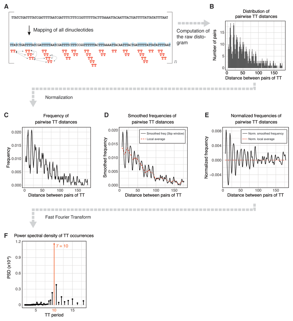
Figure 1. Estimation of k-mer power spectral density with periodicDNA.

(A) The k-mer of interest is mapped in the input sequence and all pairwise distances are calculated. (B) The distribution of all resulting pairwise distances (also called the "distogram") is generated. (C) The distogram is transformed into a frequency histogram and (D) smoothed using a moving window of 3 to mask the universal three-base genomic periodicity¹¹. (E) To normalize the frequency for distance decay, the local average (obtained by averaging the frequency with a moving window of 10) is subtracted from the smoothed frequency. (F) Finally, the power spectral density (PSD) is estimated using a Fast Fourier Transform (F). In this example, TT shows strong 10bp periodicity.

1. The k-mer occurrences are mapped and their pairwise distances are calculated (Figure 1A).
2. The distribution of all the resulting pairwise distances (also called "distogram") is generated (Figure 1B).
3. The distogram is transformed into a frequency histogram (Figure 1C) and smoothed using a moving window of 3 to mask the universal three-base genomic periodicity¹¹ (Figure 1D). To normalize the frequency for distance decay, the local average (obtained by averaging the frequency with a moving window of 10) is subtracted from the smoothed frequency (Figure 1E).
4. Finally, the power spectral density (PSD) is estimated using a Fast Fourier Transform (Figure 1F). The magnitude of the PSD values indicates the contribution of a given period to the overall periodicity of the k-mer of interest. In Figure 1, TT dinucleotides are generally 10bp periodic.

The package relies on BSGenome packages to handle genome assemblies. Genomic loci can be imported from BED files with rtracklayer and are handled in R by the GenomicRanges classes. Biostrings functions are used to map k-mer occurrences in sequences of interest.

Workflow

Installation

To install the current release of periodicDNA from Bioconductor, use:

 > if (!requireNamespace("BiocManager", quietly = TRUE))
     install.packages("BiocManager")
 > BiocManager::install("periodicDNA")
 > library("periodicDNA")

Alternatively, the developing branch of periodicDNA can be installed from Github as follows:

 > remotes::install_github("js2264/periodicDNA")
 > library("periodicDNA")

Quantifying k-mer periodicity over a set of sequences

Using a provided k-mer (e.g. WW, motif argument) and a set of sequences of interest (seqs argument), getPeriodicity() computes several different metrics:

1. The k-mer power spectral density (PSD) values at different periods obtained by Fourier Transform (following the approach described in the Implementation section). For each individual period T, the corresponding PSD_T indicates the relative contribution of the period to the overall periodicity of the k-mer of interest¹⁰.
2. The log2 fold-change, for each individual period T, between the observed PSD_T and the median of the PSD_T values measured after shuffling n times the input sequences $(l 2 F C = l o g 2 (\frac{P S D_{T, o b s e r v e d}}{m e d i a n (P S D_{T, s h u f f l e d})})) .$
3. Associated empirical p-values and false discovery rates (FDR) indicating, for each individual period T, whether the observed PSD_T,observed is significantly greater than PSD_T,shuffled values measured after shuffling n times the input sequences $(p = \frac{\sum_{i = 1}^{n} (P S D_{T, s h u f f l e d} \geq P S D_{T, o b s e r v e d}) + 1}{n + 1},$ ¹²). Note that empirical p-values are only an estimation of the real p-value. Notably, small p-values are systematically over-estimated as their lower bound is 1/(n + 1).

These metrics are accessible in the periodicityMetrics table obtained when running getPeriodicity(). For each Frequency (or Period) analysed by Fourier Transform, the resulting PSD value, a log2 fold-change, its associated p-value as well as its false-discovery rate (FDR) are returned (see tables in the examples below).

We ran getPeriodicity() on a set of 6,533 300-bp long sequences centered at all S. cerevisiae TSSs, to investigate WW periodicity, comparing to 500 shufflings as default. Using 12 cores in parallel, this function took approximately 15 minutes to run. The results were then plotted using plotPeriodicityResults() (Figure 2A), demonstrating the known underlying 10-bp WW periodicity present at promoter sequences in the yeast genome¹³.

 > # --------- Get the sequences of S. cerevisiae TSSs
 > library(TxDb.Scerevisiae.UCSC.sacCer3.sgdGene)
 > library(GenomicFeatures)
 > library(magrittr)
 > genes <- genes(TxDb.Scerevisiae.UCSC.sacCer3.sgdGene)
 > sacCer3_TSSs <- genes %>%
     resize(fix = 'center', 300) %>% 
     '['(. %within% GRanges(seqinfo(genes)))
 > # --------- Run getPeriodicity()
 > sacCer3_results <- getPeriodicity(
     sacCer3_TSSs,
     genome = 'sacCer3', 
     motif = 'WW', 
     n_shuffling = 500, 
     cores_shuffling = 12
   )
 > # --------- Plot results with plotPeriodicityResults()
 > plotPeriodicityResults(sacCer3_results, xlim = 150) 
 > # --------- Print the computed periodicity metrics 
 > sacCer3_results$periodicityMetrics

##  |  Freq|  Period|PSD_observed |    l2FC|  pval   |    fdr|
##  |-----:|-------:|:------------|-------:|:--------|------:|
##  | 0.005| 200.000|3.32e-08     | -0.5313|1.00e+00 | 1.0000|
##  | 0.010| 100.000|5.83e-09     | -0.6259|1.00e+00 | 1.0000|
##  | 0.015|  66.667|1.45e-09     | -0.7594|1.00e+00 | 1.0000|
##  | 0.020|  50.000|9.38e-10     |  0.3728|2.55e-01 | 0.9125|
##  | 0.025|  40.000|1.78e-10     | -0.7144|7.49e-01 | 1.0000|
##  | 0.030|  33.333|3.18e-10     |  0.4657|3.25e-01 | 1.0000|
##  | 0.035|  28.571|1.18e-10     | -0.9550|7.31e-01 | 1.0000|
##  | 0.040|  25.000|3.84e-11     | -2.5141|9.28e-01 | 1.0000|
##  | 0.045|  22.222|6.63e-12     | -4.9433|9.88e-01 | 1.0000|
##  | 0.050|  20.000|3.66e-11     | -1.9689|8.70e-01 | 1.0000|
##  | 0.055|  18.182|2.49e-11     | -2.6349|8.94e-01 | 1.0000|
##  | 0.060|  16.667|3.40e-10     |  1.4118|1.50e-01 | 0.7879|
##  | 0.065|  15.385|9.89e-11     | -0.3535|6.01e-01 | 1.0000|
##  | 0.070|  14.286|1.27e-11     | -3.2144|9.42e-01 | 1.0000|
##  | 0.075|  13.333|1.29e-11     | -3.2219|9.52e-01 | 1.0000|
##  | 0.080|  12.500|4.05e-10     |  1.8788|8.38e-02 | 0.5240|
##  | 0.085|  11.765|5.45e-10     |  2.4637|2.59e-02 | 0.2162|
##  | 0.090|  11.111|4.66e-11     | -0.9672|7.21e-01 | 1.0000|
##  | 0.095|  10.526|9.78e-10     |  3.5220|2.00e-03 | 0.0499|
##  | 0.100|  10.000|3.48e-09     |  5.7209|2.00e-03 | 0.0499|
##  | 0.105|   9.524|1.34e-09     |  4.3497|2.00e-03 | 0.0499|
##  | 0.110|   9.091|1.28e-10     |  1.1208|2.22e-01 | 0.8862|
##  | 0.115|   8.696|2.37e-10     |  2.1408|4.19e-02 | 0.3224|
##  | 0.120|   8.333|4.38e-10     |  3.2951|3.99e-03 | 0.0544|
##  | 0.125|   8.000|3.65e-10     |  3.0512|3.99e-03 | 0.0544|
##  | 0.130|   7.692|3.37e-10     |  3.0458|5.99e-03 | 0.0544|
##  | 0.135|   7.407|7.23e-12     | -2.5883|8.96e-01 | 1.0000|
##  | 0.140|   7.143|1.84e-11     | -1.2455|7.11e-01 | 1.0000|
##  | 0.145|   6.897|1.35e-10     |  1.7676|9.38e-02 | 0.5518|
##  | 0.150|   6.667|3.43e-11     | -0.0344|5.05e-01 | 1.0000|
##  ...

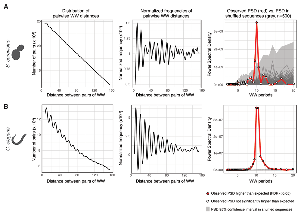
Figure 2. Output of the plotPeriodicityResults() function run on getPeriodicity() results.

To identify periodicity of WW dinucleotides, getPeriodicity() was run on (A) a set of 300-bp long sequences centered at 6,533 S. cerevisiae TSSs and (B) a set of 300-bp long sequences centered at 2,295 ubiquitous C. elegans TSSs¹⁴. The plotPeriodicityResults() function was run on the getPeriodicity() results to generate three plots as shown. Left, frequency histogram of distribution of pairwise WW distances; middle, normalised frequency histogram of distribution of pairwise WW distances; right, power spectral densities (PSDs) of a set of experimental sequences (red) and 500 iterations of shuffled sequences (grey). Grey ribbon represents the 95% confidence interval of the PSD values obtained after sequence shuffling. Red-filled dots represent PSD values in experimental sequences statistically higher than those from shuffled sequences (FDR < 0.05).

Using the same approach, we measured the WW periodicity around ubiquitous TSSs in C. elegans, which have been characterized as largely enriched for WW 10-bp periodic sequences¹⁴ (Figure 2B). The 10-bp WW periodicity at ubiquitous C. elegans TSSs is stronger than at all S. cerevisiae TSSs.

 > # ---------  Run getPeriodicity()
 > data(ce11_TSSs)
 > ce11_results <- getPeriodicity(
     ce11_TSSs[['Ubiq.']],
     genome = 'ce11', 
     motif = 'WW', 
     n_shuffling = 500, 
     cores_shuffling = 12
   )
 > # --------- Plot results with plotPeriodicityResults()
 > plotPeriodicityResults(ce11_results, xlim = 150)
 > # --------- Print the computed periodicity metrics 
 > ce11_results$periodicityMetrics

## | Freq|   Period|PSD_observed |    l2FC|  pval   |    fdr|
## |-----:|-------:|:------------|-------:|:--------|------:|
## | 0.005| 200.000|4.59e-08     |  0.0716|1.04e-01 | 0.2414|
## | 0.010| 100.000|8.96e-09     |  0.1241|2.02e-01 | 0.3733|
## | 0.015| 66.667|8.15e-10      | -1.4410|1.00e+00 | 1.0000|
## | 0.020| 50.000|3.07e-09      |  2.2148|2.00e-03 | 0.0080|
## | 0.025| 40.000|4.48e-09      |  3.7005|2.00e-03 | 0.0080|
## | 0.030| 33.333|1.59e-09      |  2.5195|5.99e-03 | 0.0222|
## | 0.035| 28.571|1.05e-09      |  1.8486|7.78e-02 | 0.2162|
## | 0.040| 25.000|2.88e-10      |  0.0116|4.95e-01 | 0.6770|
## | 0.045| 22.222|1.55e-10      | -1.0142|7.29e-01 | 0.8471|
## | 0.050| 20.000|5.22e-09      |  4.2517|2.00e-03 | 0.0080|
## | 0.055| 18.182|2.18e-10      | -0.2869|5.51e-01 | 0.7155|
## | 0.060| 16.667|3.16e-09      |  3.6181|2.00e-03 | 0.0080|
## | 0.065| 15.385|5.03e-09      |  4.4401|2.00e-03 | 0.0080|
## | 0.070| 14.286|6.47e-09      |  4.6155|2.00e-03 | 0.0080|
## | 0.075| 13.333|1.12e-08      |  5.6508|2.00e-03 | 0.0080|
## | 0.080| 12.500|2.79e-08      |  6.9992|2.00e-03 | 0.0080|
## | 0.085| 11.765|5.27e-08      |  8.0068|2.00e-03 | 0.0080|
## | 0.090| 11.111|8.08e-08      |  8.7938|2.00e-03 | 0.0080|
## | 0.095| 10.526|3.71e-07      | 10.9426|2.00e-03 | 0.0080|
## | 0.100| 10.000|3.72e-07      | 11.3303|2.00e-03 | 0.0080|
## | 0.105|  9.524|6.26e-08      |  8.8359|2.00e-03 | 0.0080|
## | 0.110|  9.091|3.56e-08      |  8.3330|2.00e-03 | 0.0080|
## | 0.115|  8.696|1.75e-08      |  7.4185|2.00e-03 | 0.0080|
## | 0.120|  8.333|7.48e-09      |  6.6215|2.00e-03 | 0.0080|
## | 0.125|  8.000|7.21e-09      |  6.4817|2.00e-03 | 0.0080|
## | 0.130|  7.692|1.43e-09      |  4.1824|2.00e-03 | 0.0080|
## | 0.135|  7.407|1.75e-09      |  4.5476|2.00e-03 | 0.0080|
## | 0.140|  7.143|8.75e-10      |  3.5609|2.00e-03 | 0.0080|
## | 0.145|  6.897|1.04e-09      |  3.7575|2.00e-03 | 0.0080|
## | 0.150|  6.667|4.38e-10      |  2.6277|1.40e-02 | 0.0466|
##  ....

Generating tracks of k-mer periodicity

The generatePeriodicityTrack() function calculates the strength of a given k-mer at a particular periodicity across genomic regions of interest, generating a linear genomic track in .bigWig format (Figure 3). The user specifies a genome and a set of genomic loci, a motif and a period of interest, and a sliding window size (window_size, 100 bp by default) and step value (step_size, 2 bp by default). The input genomic loci are split into small sliding windows and for each window, the k-mer periodicity is quantified as described in the Implementation section. The PSD value at the period of interest (e.g. period = 10) is then retrieved and assigned to the center of the corresponding window. Finally, the resulting .bigwig track is smoothed using a rolling window (smooth_track = 20). generatePeriodicityTrac() should be run in parallel across many cores using the BPPARAM argument from BiocParallel. Using 12 cores, this command takes approximately half a day to produce a periodicity track over ~ 15,000 1-kb-long GRanges with default parameters.

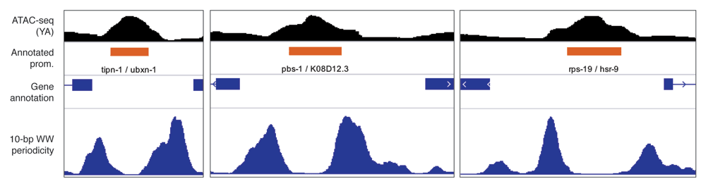
Figure 3. Example of WW dinucleotide 10-bp periodicity track at promoters in C. elegans.

ATAC-seq signal and 10-bp WW dinucleotide periodicity at three C. elegans promoters. 10bp WW dinucleotide periodicity signal was generated at 1 kb centered at annotated C. elegans promoters¹⁴ using the `generatePeriodicityTrack()` function. The data are vizualised using IGV.

As an example, we generated a WW 10-bp periodicity linear track over annotated promoters in C. elegans genome. In the previous section, we have shown that sequences in the vicinity of ubiquitous TSSs were statistically enriched for WW 10-bp periodicity. Here, the .bigwig track highlights the increased WW 10-bp periodicity in the sequences immediately flanking ubiquitous promoters, where the -1 and +1 nucleosomes are positioned¹⁴.

 > data(ce11_proms)
 > track <- getPeriodicityTrack(
     genome = 'ce11',
     granges = ce11_proms, 
     motif = 'WW',
     period = 10,
     window_size = 100,
     step_size = 2,
     smooth_track = 20,
     BPPARAM = setUpBPPARAM(12), 
     bw_file = 'WW-10-bp-periodicity_over-proms_ce11.bw'
   )

Conclusion

periodicDNA is an R package that provides functions to investigate the periodicity of k-mers of interest in DNA sequences. It is primarily designed to analyse individual or sets of sequences (typically few hundred bases long and up to a kilobase) to identify overall periodicity of a chosen k-mer. It can also generate linear .bigwig tracks of k-mer periodicity at a chosen period (e.g. 10-bp WW periodicity), over genomic loci of interest. periodicDNA is well integrated within the Bioconductor environment and can easily fit in standard genomic analysis workflows.

Data availability

Underlying data

This project contains underlying data published in Serizay et al., 2020¹⁴. All the data are also available from the original reference.

Software availability

periodicDNA is released as an R package on Bioconductor: http://www.bioconductor.org/packages/release/bioc/html/periodicDNA.html

Source code available from: https://github.com/js2264/periodicDNA.

Archived source code as at time of publication: https://doi.org/10.5281/zenodo.4533704¹⁵.

License: GPL-3

Acknowledgments

We would like to thank T. Winder for his help interpreting Fourier Transform analyses.

Faculty Opinions recommended

References

1. Xiong H, Buckwalter BL, Shieh HM, et al.: Periodicity of polar and nonpolar amino acids is the major determinant of secondary structure in self-assembling oligomeric peptides. Proc Natl Acad Sci U S A. 1995; 92(14): 6349–53. PubMed Abstract | Publisher Full Text | Free Full Text
2. Korotkova MA, Korotkov EV, Rudenko VM: Latent Periodicity of Protein Sequences. Molecular Modeling Annual. 1999; 5(6): 103–15. Publisher Full Text
3. Trotta E: The 3-base periodicity and codon usage of coding sequences are correlated with gene expression at the level of transcription elongation. PLoS One. 2011; 6(6): e21590. PubMed Abstract | Publisher Full Text | Free Full Text
4. Frenkel FE, Korotkova MA, Korotkov EV: Database of Periodic DNA Regions in Major Genomes. Biomed Res Int. 2017; 2017: 7949287. PubMed Abstract | Publisher Full Text | Free Full Text
5. Eskesen ST, Eskesen FN, Kinghorn B, et al.: Periodicity of DNA in exons. BMC Mol Biol. 2004; 5: 12. PubMed Abstract | Publisher Full Text | Free Full Text
6. Travers A, Hiriart E, Churcher M, et al.: The DNA sequence-dependence of nucleosome positioning in vivo and in vitro. J Biomol Struct Dyn. 2010; 27(6): 713–24. PubMed Abstract | Publisher Full Text | Free Full Text
7. Struhl K, Segal E: Determinants of nucleosome positioning. Nat Struct Mol Biol. 2013; 20(3): 267–73. PubMed Abstract | Publisher Full Text | Free Full Text
8. Larsson E, Lindahl P, Mostad P: HeliCis: a DNA motif discovery tool for colocalized motif pairs with periodic spacing. BMC Bioinformatics. 2007; 8(1): 418. PubMed Abstract | Publisher Full Text | Free Full Text
9. Whitington T, Frith MC, Johnson J, et al.: Inferring transcription factor complexes from ChIP-seq data. Nucleic Acids Res. 2011; 39(15): e98. PubMed Abstract | Publisher Full Text | Free Full Text
10. Yin C, Wang J: Periodic power spectrum with applications in detection of latent periodicities in DNA sequences. J Math Biol. 2016; 73(5): 1053–79. PubMed Abstract | Publisher Full Text
11. Howe ED, Song JS: Categorical spectral analysis of periodicity in human and viral genomes. Nucleic Acids Res. 2013; 41(3): 1395–405. PubMed Abstract | Publisher Full Text | Free Full Text
12. North BV, Curtis D, Sham PC: A note on calculation of empirical P values from Monte Carlo procedure. Am J Hum Genet. 2003; 72(2): 498–9. PubMed Abstract | Publisher Full Text | Free Full Text
13. Mavrich TN, Ioshikhes IP, Venters BJ, et al.: A barrier nucleosome model for statistical positioning of nucleosomes throughout the yeast genome. Genome Res. 2008; 18(7): 1073–83. PubMed Abstract | Publisher Full Text | Free Full Text
14. Serizay J, Dong Y, Jänes J, et al.: Distinctive regulatory architectures of germline-active and somatic genes in C. elegans. Genome Res. 2020; 30(12): 1752–65. PubMed Abstract | Publisher Full Text | Free Full Text
15. Serizay J: periodicDNA (Version 1.0.0). Zenodo. 2021. http://www.doi.org/10.5281/zenodo.4533704

Comments on this article Comments (0)

Version 1

VERSION 1 PUBLISHED 24 Feb 2021

Author details Author details

¹ The Gurdon Institute and Department of Genetics, University of Cambridge, Cambridge, CB2 1QN, UK

Jacques Serizay
Roles: Conceptualization, Data Curation, Formal Analysis, Investigation, Methodology, Software, Validation, Visualization, Writing – Original Draft Preparation, Writing – Review & Editing

Julie Ahringer
Roles: Conceptualization, Funding Acquisition, Supervision, Writing – Original Draft Preparation, Writing – Review & Editing

Competing interests

No competing interests were disclosed.

Grant information

The work was supported by a Wellcome Trust Senior Research Fellowship to J.A. (101863) and a Medical Research Council DTP studentship to J.S..
The funders had no role in study design, data collection and analysis, decision to publish, or preparation of the manuscript.

Article Versions (1)

version 1

Published: 24 Feb 2021, 10:141

https://doi.org/10.12688/f1000research.51143.1

Copyright

© 2021 Serizay J and Ahringer J. This is an open access article distributed under the terms of the Creative Commons Attribution License, which permits unrestricted use, distribution, and reproduction in any medium, provided the original work is properly cited.

Download

Export To

metrics

	Views	Downloads
F1000Research	-	-
PubMed Central Data from PMC are received and updated monthly.	-	-

Citations

0

SEE MORE DETAILS

CITE

how to cite this article

Serizay J and Ahringer J. periodicDNA: an R/Bioconductor package to investigate k-mer periodicity in DNA [version 1; peer review: 1 approved, 3 approved with reservations]. F1000Research 2021, 10:141 (https://doi.org/10.12688/f1000research.51143.1)

NOTE: If applicable, it is important to ensure the information in square brackets after the title is included in all citations of this article.

track

receive updates on this article

Track an article to receive email alerts on any updates to this article.

Open Peer Review

Current Reviewer Status: ?

Key to Reviewer Statuses VIEW HIDE

ApprovedThe paper is scientifically sound in its current form and only minor, if any, improvements are suggested

Approved with reservations A number of small changes, sometimes more significant revisions are required to address specific details and improve the papers academic merit.

Not approvedFundamental flaws in the paper seriously undermine the findings and conclusions

Version 1

VERSION 1

PUBLISHED 24 Feb 2021

Views

14

Reviewer Report 12 May 2021

Boris Lenhard, Institute of Clinical Sciences, Faculty of Medicine, Imperial College London, London, UK

Approved with Reservations

https://doi.org/10.5256/f1000research.54274.r80117

periodicDNA is a R/Bioconductor package for the detection and visualisation of string-based periodic motifs (k-mers) in DNA sequences. While there are several periodic motifs that are known to occur in genomic sentences, the paper - and, for the most part, ... Continue reading

periodicDNA is a R/Bioconductor package for the detection and visualisation of string-based periodic motifs (k-mers) in DNA sequences. While there are several periodic motifs that are known to occur in genomic sentences, the paper - and, for the most part, the tool itself - focuses on the analysis of by far the most important of them, the 10-bp periodicity of WW dinucleotides that is the hallmark of nucleosome positioning signals, present in the majority of RNA polymerase II promoters, in most eukaryotic genomes analysed so far.

The tool implements the calculation of power spectral density over the distances between the instances of k-mers in a set of sequences by normalising the frequencies of pairwise TT distances against "smoothed" distances. It has only a couple of main functions, one for performing general power spectrum analyses, with table of power spectral density as a result, and one that produces a genome browser track for a selected set of sequences using a predefined period size. The latter is shown to produce a characteristic double pattern at bidirectional promoters in C. elegans (Figure 3).

The tool is simple, clean, and seems to do its job well. I have only a couple of suggestions:

The smoothed local average (Figure 1D) uses a 10 bp window. While that is a suitable window size for nucleosome positioning signal, it might not work for exploring other, possibly unknown periodic motifs. It should at least be remarked on, and the authors should consider adding functionality to suggest an optimal or at least minimal window size for averaging.
The stated running times on a 12-core CPU for the presented examples look surprisingly long to me. Could the authors provide more detail - with or without profiling the code - about which computational step is the reason the whole calculation takes this long?

Is the rationale for developing the new software tool clearly explained?

Yes
Is the description of the software tool technically sound?

Yes
Are sufficient details of the code, methods and analysis (if applicable) provided to allow replication of the software development and its use by others?

Partly
Is sufficient information provided to allow interpretation of the expected output datasets and any results generated using the tool?

Yes
Are the conclusions about the tool and its performance adequately supported by the findings presented in the article?

Yes

Competing Interests: No competing interests were disclosed.

Reviewer Expertise: Gene regulation.

I confirm that I have read this submission and believe that I have an appropriate level of expertise to confirm that it is of an acceptable scientific standard, however I have significant reservations, as outlined above.

CITE

Report a concern

Respond or Comment

Views

18

Reviewer Report 13 Apr 2021

Eugene Korotkov, Research Center of Biotechnology, Russian Academy of Sciences, Moscow, Russian Federation

Approved with Reservations

https://doi.org/10.5256/f1000research.54274.r81592

The manuscript is aimed at solving an important problem - the study of the structure of promoter sequences. The calculations are performed at a good scientific level, the results are beyond doubt. I have only three, as it seems to ... Continue reading

The manuscript is aimed at solving an important problem - the study of the structure of promoter sequences. The calculations are performed at a good scientific level, the results are beyond doubt. I have only three, as it seems to me, small comments.

1. It seems to me that it is not entirely correct to represent the data as a file printout. Probably it would be better to present this data in the form of tables.

2. Figure 3 evokes some skepticism. It seems to me that it is very difficult to draw a conclusion on 3 promoters. Maybe this is a purely coincidence. I believe that it is necessary to study much more promoters in this way in order to draw any conclusions. Probably more promoter sequences need to be studied.

3. There are a lot of publications on the search for periodicity in promoter sequences. For example, Kravatskaya GI et al. (2011)¹ and Nov Klaiman T et al. (2009)²

It seems to me that a little comparative analysis could be done in the discussion.

Is the rationale for developing the new software tool clearly explained?

Yes
Is the description of the software tool technically sound?

Yes
Are sufficient details of the code, methods and analysis (if applicable) provided to allow replication of the software development and its use by others?

Yes
Is sufficient information provided to allow interpretation of the expected output datasets and any results generated using the tool?

Yes
Are the conclusions about the tool and its performance adequately supported by the findings presented in the article?

Partly

References

1. Kravatskaya GI, Kravatsky YV, Chechetkin VR, Tumanyan VG: Coexistence of different base periodicities in prokaryotic genomes as related to DNA curvature, supercoiling, and transcription.Genomics. 2011; 98 (3): 223-31 PubMed Abstract | Publisher Full Text
2. Nov Klaiman T, Hosid S, Bolshoy A: Upstream curved sequences in E. coli are related to the regulation of transcription initiation.Comput Biol Chem. 2009; 33 (4): 275-82 PubMed Abstract | Publisher Full Text

Competing Interests: No competing interests were disclosed.

Reviewer Expertise: Bioinformatics

I confirm that I have read this submission and believe that I have an appropriate level of expertise to confirm that it is of an acceptable scientific standard, however I have significant reservations, as outlined above.

CITE

Report a concern

Respond or Comment

Views

18

Reviewer Report 12 Apr 2021

Sabarinathan Radhakrishnan, National Centre for Biological Sciences, Bangalore, India

Approved

https://doi.org/10.5256/f1000research.54274.r81589

The manuscript by Serizay and Ahringer presents an R/Bioconductor package to investigate the k-mer periodicity in DNA. Both the manuscript and the package details are informative and will be useful to the researchers. The following are some minor comments and ... Continue reading

The manuscript by Serizay and Ahringer presents an R/Bioconductor package to investigate the k-mer periodicity in DNA. Both the manuscript and the package details are informative and will be useful to the researchers. The following are some minor comments and suggestions:

a) Regarding the shuffling of input sequences, it is not clear if there is an option to preserve the doublet or triplet nucleotide counts. Is the parameter “order” in getPeriodicity() function meant for that (through ushuffle)? If so, please do mention this in the manuscript and its default value.

b) In addition to the shuffling of input sequences, it would also be useful if the function allows for random selection of N number of sequences (with similar GC content) from the genome or an option for the users to define their own set of input random sequences (through DNAstringSet or bed file).

c) In Figure 1A, under the “Mapping of all dinucleotides” it is not clear why the single occurrence of ‘T’ is also shaded.

Is the rationale for developing the new software tool clearly explained?

Yes
Is the description of the software tool technically sound?

Yes
Are sufficient details of the code, methods and analysis (if applicable) provided to allow replication of the software development and its use by others?

Yes
Is sufficient information provided to allow interpretation of the expected output datasets and any results generated using the tool?

Yes
Are the conclusions about the tool and its performance adequately supported by the findings presented in the article?

Yes

Competing Interests: No competing interests were disclosed.

Reviewer Expertise: Bioinformatics, Cancer genomics, mutational processes and gene regulation.

I confirm that I have read this submission and believe that I have an appropriate level of expertise to confirm that it is of an acceptable scientific standard.

CITE

Report a concern

Respond or Comment

Views

26

Reviewer Report 26 Mar 2021

Ilya Ioshikhes, University of Ottawa, Ottawa, Canada

Approved with Reservations

https://doi.org/10.5256/f1000research.54274.r81590

The software offered is potentially helpful to the researchers in the area. However the paper (and probably the software itself) should be modified to enable its complete evaluation for indexing.

Comparison to other existing state of

The software offered is potentially helpful to the researchers in the area. However the paper (and probably the software itself) should be modified to enable its complete evaluation for indexing.

Comparison to other existing state of the art approaches should be added, e.g. to PerPlot and PerScan tools by Mrazek and colleagues¹, ID/MPA by Shelenkov et al., 2008². The progress obtained in the present submission should be clarified.
All the examples shown in the paper and related links are focused on TT dinucleotides. It is not clear whether oligo nucleotide combinations involving W, S, R, Y, N, and others from the IUPAC nucleotide codes are supported by the present software version.
It is not clear whether there any other restrictions on the software parameters, e.g. oligonucleotide and sequences lengths.
The software is composed at R language with key functions provided. To make it really practically helpful, the graphic user interface should be provided, to enable entering oligonucleotides of interest and other parameters from a window or dialogue line, without necessitating the changes in the functions text. As a very minimum, the clear instructions for such changes should be provided.

Is the rationale for developing the new software tool clearly explained?

Yes
Is the description of the software tool technically sound?

Yes
Are sufficient details of the code, methods and analysis (if applicable) provided to allow replication of the software development and its use by others?

Yes
Is sufficient information provided to allow interpretation of the expected output datasets and any results generated using the tool?

Yes
Are the conclusions about the tool and its performance adequately supported by the findings presented in the article?

Yes

References

1. Mrázek J, Chaudhari T, Basu A: PerPlot & PerScan: tools for analysis of DNA curvature-related periodicity in genomic nucleotide sequences.Microb Inform Exp. 2011; 1 (1): 13 PubMed Abstract | Publisher Full Text
2. Shelenkov A, Skryabin K, Korotkov E: Classification analysis of a latent dinucleotide periodicity of plant genomes. Russian Journal of Genetics. 2008; 44 (1): 101-114 Publisher Full Text

Competing Interests: No competing interests were disclosed.

Reviewer Expertise: Bioinformatics, gene regulation, nucleosomes, algorithms

I confirm that I have read this submission and believe that I have an appropriate level of expertise to confirm that it is of an acceptable scientific standard, however I have significant reservations, as outlined above.

CITE

Report a concern

Respond or Comment

Comments on this article Comments (0)

Version 1

VERSION 1 PUBLISHED 24 Feb 2021

Open Peer Review

Reviewer Status

Reviewer Reports

	Invited Reviewers
	1	2	3	4
Version 1 24 Feb 21	read	read	read	read

Ilya Ioshikhes, University of Ottawa, Ottawa, Canada
Sabarinathan Radhakrishnan, National Centre for Biological Sciences, Bangalore, India
Eugene Korotkov, Russian Academy of Sciences, Moscow, Russian Federation
Boris Lenhard, Imperial College London, London, UK

Comments on this article

All Comments(0)

Add a comment

Sign up for content alerts

Browse by related subjects

Back to all reports

Reviewer Report

14 Views

12 May 2021 | for Version 1

Boris Lenhard, Institute of Clinical Sciences, Faculty of Medicine, Imperial College London, London, UK

14 Views Cite this report Responses(0)

Approved With Reservations

periodicDNA is a R/Bioconductor package for the detection and visualisation of string-based periodic motifs (k-mers) in DNA sequences. While there are several periodic motifs that are known to occur in genomic sentences, the paper - and, for the most part, the tool itself - focuses on the analysis of by far the most important of them, the 10-bp periodicity of WW dinucleotides that is the hallmark of nucleosome positioning signals, present in the majority of RNA polymerase II promoters, in most eukaryotic genomes analysed so far.

The tool implements the calculation of power spectral density over the distances between the instances of k-mers in a set of sequences by normalising the frequencies of pairwise TT distances against "smoothed" distances. It has only a couple of main functions, one for performing general power spectrum analyses, with table of power spectral density as a result, and one that produces a genome browser track for a selected set of sequences using a predefined period size. The latter is shown to produce a characteristic double pattern at bidirectional promoters in C. elegans (Figure 3).

The tool is simple, clean, and seems to do its job well. I have only a couple of suggestions:

The smoothed local average (Figure 1D) uses a 10 bp window. While that is a suitable window size for nucleosome positioning signal, it might not work for exploring other, possibly unknown periodic motifs. It should at least be remarked on, and the authors should consider adding functionality to suggest an optimal or at least minimal window size for averaging.
The stated running times on a 12-core CPU for the presented examples look surprisingly long to me. Could the authors provide more detail - with or without profiling the code - about which computational step is the reason the whole calculation takes this long?

Is the rationale for developing the new software tool clearly explained?

Yes
Is the description of the software tool technically sound?

Yes
Are sufficient details of the code, methods and analysis (if applicable) provided to allow replication of the software development and its use by others?

Partly
Is sufficient information provided to allow interpretation of the expected output datasets and any results generated using the tool?

Yes
Are the conclusions about the tool and its performance adequately supported by the findings presented in the article?

Yes

Competing Interests

No competing interests were disclosed.

Reviewer Expertise

Gene regulation.

I confirm that I have read this submission and believe that I have an appropriate level of expertise to confirm that it is of an acceptable scientific standard, however I have significant reservations, as outlined above.

Respond to this report

Responses (0)

Back to all reports

Reviewer Report

18 Views

13 Apr 2021 | for Version 1

Eugene Korotkov, Research Center of Biotechnology, Russian Academy of Sciences, Moscow, Russian Federation

18 Views Cite this report Responses(0)

Approved With Reservations

The manuscript is aimed at solving an important problem - the study of the structure of promoter sequences. The calculations are performed at a good scientific level, the results are beyond doubt. I have only three, as it seems to me, small comments.

1. It seems to me that it is not entirely correct to represent the data as a file printout. Probably it would be better to present this data in the form of tables.

2. Figure 3 evokes some skepticism. It seems to me that it is very difficult to draw a conclusion on 3 promoters. Maybe this is a purely coincidence. I believe that it is necessary to study much more promoters in this way in order to draw any conclusions. Probably more promoter sequences need to be studied.

3. There are a lot of publications on the search for periodicity in promoter sequences. For example, Kravatskaya GI et al. (2011)¹ and Nov Klaiman T et al. (2009)²

It seems to me that a little comparative analysis could be done in the discussion.

Is the rationale for developing the new software tool clearly explained?

Yes
Is the description of the software tool technically sound?

Yes
Are sufficient details of the code, methods and analysis (if applicable) provided to allow replication of the software development and its use by others?

Yes
Is sufficient information provided to allow interpretation of the expected output datasets and any results generated using the tool?

Yes
Are the conclusions about the tool and its performance adequately supported by the findings presented in the article?

Partly

References

1. Kravatskaya GI, Kravatsky YV, Chechetkin VR, Tumanyan VG: Coexistence of different base periodicities in prokaryotic genomes as related to DNA curvature, supercoiling, and transcription.Genomics. 2011; 98 (3): 223-31 PubMed Abstract | Publisher Full Text
2. Nov Klaiman T, Hosid S, Bolshoy A: Upstream curved sequences in E. coli are related to the regulation of transcription initiation.Comput Biol Chem. 2009; 33 (4): 275-82 PubMed Abstract | Publisher Full Text

Competing Interests

No competing interests were disclosed.

Reviewer Expertise

Bioinformatics

I confirm that I have read this submission and believe that I have an appropriate level of expertise to confirm that it is of an acceptable scientific standard, however I have significant reservations, as outlined above.

Respond to this report

Responses (0)

Back to all reports

Reviewer Report

18 Views

12 Apr 2021 | for Version 1

Sabarinathan Radhakrishnan, National Centre for Biological Sciences, Bangalore, India

18 Views Cite this report Responses(0)

Approved

The manuscript by Serizay and Ahringer presents an R/Bioconductor package to investigate the k-mer periodicity in DNA. Both the manuscript and the package details are informative and will be useful to the researchers. The following are some minor comments and suggestions:

a) Regarding the shuffling of input sequences, it is not clear if there is an option to preserve the doublet or triplet nucleotide counts. Is the parameter “order” in getPeriodicity() function meant for that (through ushuffle)? If so, please do mention this in the manuscript and its default value.

b) In addition to the shuffling of input sequences, it would also be useful if the function allows for random selection of N number of sequences (with similar GC content) from the genome or an option for the users to define their own set of input random sequences (through DNAstringSet or bed file).

c) In Figure 1A, under the “Mapping of all dinucleotides” it is not clear why the single occurrence of ‘T’ is also shaded.

Is the rationale for developing the new software tool clearly explained?

Yes
Is the description of the software tool technically sound?

Yes
Are sufficient details of the code, methods and analysis (if applicable) provided to allow replication of the software development and its use by others?

Yes
Is sufficient information provided to allow interpretation of the expected output datasets and any results generated using the tool?

Yes
Are the conclusions about the tool and its performance adequately supported by the findings presented in the article?

Yes

Competing Interests

No competing interests were disclosed.

Reviewer Expertise

Bioinformatics, Cancer genomics, mutational processes and gene regulation.

I confirm that I have read this submission and believe that I have an appropriate level of expertise to confirm that it is of an acceptable scientific standard.

Respond to this report

Responses (0)

Back to all reports

Reviewer Report

26 Views

26 Mar 2021 | for Version 1

Ilya Ioshikhes, University of Ottawa, Ottawa, Canada

26 Views Cite this report Responses(0)

Approved With Reservations

The software offered is potentially helpful to the researchers in the area. However the paper (and probably the software itself) should be modified to enable its complete evaluation for indexing.

Comparison to other existing state of the art approaches should be added, e.g. to PerPlot and PerScan tools by Mrazek and colleagues¹, ID/MPA by Shelenkov et al., 2008². The progress obtained in the present submission should be clarified.
All the examples shown in the paper and related links are focused on TT dinucleotides. It is not clear whether oligo nucleotide combinations involving W, S, R, Y, N, and others from the IUPAC nucleotide codes are supported by the present software version.
It is not clear whether there any other restrictions on the software parameters, e.g. oligonucleotide and sequences lengths.
The software is composed at R language with key functions provided. To make it really practically helpful, the graphic user interface should be provided, to enable entering oligonucleotides of interest and other parameters from a window or dialogue line, without necessitating the changes in the functions text. As a very minimum, the clear instructions for such changes should be provided.

Is the rationale for developing the new software tool clearly explained?

Yes
Is the description of the software tool technically sound?

Yes
Are sufficient details of the code, methods and analysis (if applicable) provided to allow replication of the software development and its use by others?

Yes
Is sufficient information provided to allow interpretation of the expected output datasets and any results generated using the tool?

Yes
Are the conclusions about the tool and its performance adequately supported by the findings presented in the article?

Yes

References

1. Mrázek J, Chaudhari T, Basu A: PerPlot & PerScan: tools for analysis of DNA curvature-related periodicity in genomic nucleotide sequences.Microb Inform Exp. 2011; 1 (1): 13 PubMed Abstract | Publisher Full Text
2. Shelenkov A, Skryabin K, Korotkov E: Classification analysis of a latent dinucleotide periodicity of plant genomes. Russian Journal of Genetics. 2008; 44 (1): 101-114 Publisher Full Text

Competing Interests

No competing interests were disclosed.

Reviewer Expertise

Bioinformatics, gene regulation, nucleosomes, algorithms

I confirm that I have read this submission and believe that I have an appropriate level of expertise to confirm that it is of an acceptable scientific standard, however I have significant reservations, as outlined above.

Respond to this report

Responses (0)

[1] 1. Xiong H, Buckwalter BL, Shieh HM, et al.: Periodicity of polar and nonpolar amino acids is the major determinant of secondary structure in self-assembling oligomeric peptides. Proc Natl Acad Sci U S A. 1995; 92(14): 6349–53. PubMed Abstract | Publisher Full Text | Free Full Text

[2] 2. Korotkova MA, Korotkov EV, Rudenko VM: Latent Periodicity of Protein Sequences. Molecular Modeling Annual. 1999; 5(6): 103–15. Publisher Full Text

[3] 3. Trotta E: The 3-base periodicity and codon usage of coding sequences are correlated with gene expression at the level of transcription elongation. PLoS One. 2011; 6(6): e21590. PubMed Abstract | Publisher Full Text | Free Full Text

[4] 4. Frenkel FE, Korotkova MA, Korotkov EV: Database of Periodic DNA Regions in Major Genomes. Biomed Res Int. 2017; 2017: 7949287. PubMed Abstract | Publisher Full Text | Free Full Text

[5] 5. Eskesen ST, Eskesen FN, Kinghorn B, et al.: Periodicity of DNA in exons. BMC Mol Biol. 2004; 5: 12. PubMed Abstract | Publisher Full Text | Free Full Text

[6] 6. Travers A, Hiriart E, Churcher M, et al.: The DNA sequence-dependence of nucleosome positioning in vivo and in vitro. J Biomol Struct Dyn. 2010; 27(6): 713–24. PubMed Abstract | Publisher Full Text | Free Full Text

[7] 7. Struhl K, Segal E: Determinants of nucleosome positioning. Nat Struct Mol Biol. 2013; 20(3): 267–73. PubMed Abstract | Publisher Full Text | Free Full Text

[8] 8. Larsson E, Lindahl P, Mostad P: HeliCis: a DNA motif discovery tool for colocalized motif pairs with periodic spacing. BMC Bioinformatics. 2007; 8(1): 418. PubMed Abstract | Publisher Full Text | Free Full Text

[9] 9. Whitington T, Frith MC, Johnson J, et al.: Inferring transcription factor complexes from ChIP-seq data. Nucleic Acids Res. 2011; 39(15): e98. PubMed Abstract | Publisher Full Text | Free Full Text

[10] 10. Yin C, Wang J: Periodic power spectrum with applications in detection of latent periodicities in DNA sequences. J Math Biol. 2016; 73(5): 1053–79. PubMed Abstract | Publisher Full Text

[11] 11. Howe ED, Song JS: Categorical spectral analysis of periodicity in human and viral genomes. Nucleic Acids Res. 2013; 41(3): 1395–405. PubMed Abstract | Publisher Full Text | Free Full Text

[12] 12. North BV, Curtis D, Sham PC: A note on calculation of empirical P values from Monte Carlo procedure. Am J Hum Genet. 2003; 72(2): 498–9. PubMed Abstract | Publisher Full Text | Free Full Text

[13] 13. Mavrich TN, Ioshikhes IP, Venters BJ, et al.: A barrier nucleosome model for statistical positioning of nucleosomes throughout the yeast genome. Genome Res. 2008; 18(7): 1073–83. PubMed Abstract | Publisher Full Text | Free Full Text

[14] 14. Serizay J, Dong Y, Jänes J, et al.: Distinctive regulatory architectures of germline-active and somatic genes in C. elegans. Genome Res. 2020; 30(12): 1752–65. PubMed Abstract | Publisher Full Text | Free Full Text

[15] 15. Serizay J: periodicDNA (Version 1.0.0). Zenodo. 2021. http://www.doi.org/10.5281/zenodo.4533704

periodicDNA: an R/Bioconductor package to investigate k-mer periodicity in DNA

Abstract

Keywords

Introduction

Methods

Operation

Implementation

Figure 1. Estimation of k-mer power spectral density with periodicDNA.

Workflow

Installation

Quantifying k-mer periodicity over a set of sequences

Figure 2. Output of the plotPeriodicityResults() function run on getPeriodicity() results.

Generating tracks of k-mer periodicity

Figure 3. Example of WW dinucleotide 10-bp periodicity track at promoters in C. elegans.

Conclusion

Data availability

Underlying data

Software availability

Acknowledgments

References

Comments on this article Comments (0)

Open Peer Review

Comments on this article Comments (0)

Open Peer Review

Reviewer Status

Reviewer Reports

Comments on this article

Browse by related subjects

Competing Interests Policy

Stay Updated