Spatial transcriptomics dimensionality reduction using wavelet bases

Zhuoyan Xu; Kris Sankaran

doi:10.12688/f1000research.122775.1

Home Browse Spatial transcriptomics dimensionality reduction using wavelet bases

ALL Metrics

-

Views

-

Downloads

Get PDF

Get XML

Export

▬

✚

Method Article

Spatial transcriptomics dimensionality reduction using wavelet bases

[version 1; peer review: 3 approved with reservations, 1 not approved]

Zhuoyan Xu¹, Kris Sankaran¹

PUBLISHED 12 Sep 2022

Author details Author details

¹ Department of Statistics, University of Wisconsin - Madison, Madison, Wisconsin, 53706, USA

Zhuoyan Xu
Roles: Conceptualization, Data Curation, Formal Analysis, Investigation, Methodology, Project Administration, Software, Validation, Visualization, Writing – Original Draft Preparation, Writing – Review & Editing

Kris Sankaran
Roles: Conceptualization, Data Curation, Formal Analysis, Funding Acquisition, Investigation, Methodology, Project Administration, Resources, Software, Supervision, Validation, Visualization, Writing – Original Draft Preparation, Writing – Review & Editing

OPEN PEER REVIEW

REVIEWER STATUS

This article is included in the Bioinformatics gateway.

This article is included in the Artificial Intelligence and Machine Learning gateway.

This article is included in the Machine Learning in Genomics collection.

Abstract

Background: Spatially resolved transcriptomics (ST) measures gene expression along with the spatial coordinates of the measurements. The analysis of ST data involves significant computation complexity. In this work, we propose a gene expression dimensionality reduction algorithm that retains spatial structure.
Methods: We combine the wavelet transformation with matrix factorization to select spatially-varying genes. We extract a low-dimensional representation of these genes. We adopt an Empirical Bayes perspective, imposing regularization through the prior distribution of factor genes. Additionally, we visualize the extracted representations, providing an overview of global spatial patterns. We illustrate the performance of our methods through spatial structure recovery and gene expression reconstruction using a simulation and real data analysis.
Results: In real data experiments, our method identifies spatial structure of gene factors and outperforms regular decomposition regarding reconstruction error. We find a connection between the fluctuation of gene patterns and wavelet estimates, and this allows us to provide smoother visualizations. We develop the package and share the workflow generating reproducible quantitative results and gene visualization. The package is available at https://github.com/OliverXUZY/waveST.
Conclusions: We have proposed a pipeline for dimensionality reduction that respects spatial structure. Both simulations and real data experiments demonstrate that wavelet and shrinkage techniques show positive results in spatially resolved transcriptomics data. We highlight the idea of combining image processing techniques and statistical methods for application in a spatial genomics context

Keywords

Spatial Transcriptomics, Wavelet Transformation, Empirical Bayes Matrix Factorization, Factor Gene

Corresponding author: Kris Sankaran

Competing interests: No competing interests were disclosed.

Grant information: This research was performed using the compute resources and assistance of the UW-Madison Center For High Throughput Computing (CHTC) in the Department of Computer Sciences. The CHTC is supported by UW-Madison, the Advanced Computing Initiative, the Wisconsin Alumni Research Foundation, the Wisconsin Institutes for Discovery, and the National Science Foundation, and is an active member of the OSG Consortium, which is supported by the National Science Foundation and the U.S. Department of Energy’s Office of Science.
The funders had no role in study design, data collection and analysis, decision to publish, or preparation of the manuscript.

Copyright: © 2022 Xu Z and Sankaran K. This is an open access article distributed under the terms of the Creative Commons Attribution License, which permits unrestricted use, distribution, and reproduction in any medium, provided the original work is properly cited.

How to cite: Xu Z and Sankaran K. Spatial transcriptomics dimensionality reduction using wavelet bases [version 1; peer review: 3 approved with reservations, 1 not approved]. F1000Research 2022, 11:1033 (https://doi.org/10.12688/f1000research.122775.1) First published: 12 Sep 2022, 11:1033 (https://doi.org/10.12688/f1000research.122775.1) Latest published: 12 Sep 2022, 11:1033 (https://doi.org/10.12688/f1000research.122775.1)

Introduction

Spatial resolved transcriptomics (ST) is a technology measuring spatial variation in gene expression. Different technological platforms support different genome coverage and spatial resolution (tissue-level measurement to subcellular measurement). Examples of ST platforms include Spatial Transcriptomics (Ståhl et al., 2016; Xia et al., 2019), 10x Genomics Visium, Slide-seq (Rodriques et al., 2019), sci-Space (Srivatsan et al., 2021), and MERFISH (Chen et al., 2015). Spatial transcriptomics allows visualization and quantitative analysis of the transcriptome with spatial resolution in individual tissue sections. A series of studies combining gene expression and spatial information has been brought to generate new insight in biological analysis (Kuppe et al., 2020; Shah et al., 2016; Berglund et al., 2018). Quantification of gene expression has wide applications in transcriptomics. Understanding the spatial distribution of gene expression has helped to answer fundamental questions in developmental biology (Asp et al., 2019; Rödelsperger et al., 2021), cancer (Thrane et al., 2018; Moncada et al., 2020), and neuroscience (Moffitt et al., 2016; Close et al., 2021). Two widely-used methods for gene expression quantification are fluorescent in situ hybridization (FISH) and next-generation sequencing.

While these approaches have been made to measure gene expression while preserving spatial information, there are statistical challenges in analyses combining the gene and spatial information. Specifically, gene dimensionality reduction guided by spatial information is still an active area of study (Abu-Jamous and Kelly, 2018; Kiselev et al., 2017, 2018; Zhu and Sabatti, 2020; Shang and Zhou, 2022; Velten et al., 2022; Townes and Engelhardt, 2021). In this work, we conduct a dimensionality reduction on spatially varying gene data. After transformation, gene expression over locations is a square matrix, which allows us to view it as an image. Therefore, tools from image processing can be adapted – our method incorporates spatial information by wavelet transformation, a multi-scale analysis decompose sequence into orthonormal series. We apply wavelet transformation for each gene expression over locations. This is a common technique in denoising the image. We thus apply techniques analogous to image analysis. We evaluate performance using reconstruction error and comparing resulting visualizations. Our analysis pipeline builds from off-the-shelf tools, and code is available for reproducing our results. We also attach visualizations in our pipeline, giving example interpretations of intermediate result.

A natural idea in spatial transcriptomic analysis is to identify gene types across spatial locations (Abu-Jamous and Kelly, 2018). For example, in clustering the representations in each cluster achieve dimensionality reduction under the assumption that genes within one cluster have the same type. A parallel technique is clustering based on cell type instead. General clustering methods can be combined into more sophisticated pipelines tailored toward spatial single-cell analysis. SC3 (single-cell consensus clustering 3) (Kiselev et al., 2017) is an ensemble clustering method. It calculates distance matrices across cell locations using the Euclidean distance, then applies spectral clustering, and assigns membership (Kiselev et al., 2018). To identify the cell type in each cluster, one can perform differential expression analysis between all pairs of clusters. scGeneFit uses a label-aware compression method to find marker genes (Dumitrascu et al., 2021). Given the cell-by-gene expression matrix and cell clustering membership, scGeneFit maps cells to lower-dimensional space where cells within the same cluster are closer. For gene dimensionality reduction, (Zhu and Sabatti, 2020) constructs a neighborhood graph from the spatial coordinates, then applies a graph-based feature selection procedure to determine spatially varying genes. They also provide the option to infer a latent graph embedding for cells based on selected genes, applying spline models to fit the gene’s expression on the latent embedding. Then they leverage the fitted coefficients to reduce the dimensionality of each gene. (Svensson et al., 2018) proposed pipelines using mixed-effect models incorporating spatial information. The model contains two random effect terms: a spatial variance term that parametrizes gene expression covariance by pairwise distance between samples and a noise term that models nonspatial variability. The model leverages efficient inference methods previously developed for linear mixed models, and it is computationally efficient.

Our setting is closely aligned with the following recent works: (Shang and Zhou, 2022) developed SpatialPCA, applying probabilistic principal component analysis (PCA) on ST data for dimensionality reduction. They assume data are given as a location-by-genes matrix and construct a regression model similar to factor analysis, where the prior covariance matrix of factor genes is a distance matrix constructed with a Gaussian kernel. (Velten et al., 2022) proposed MEFISTO, combining factor analysis with the non-parametric framework of Gaussian processes to model spatio-temporal dependencies in the latent space. (Townes and Engelhardt, 2021) developed nonnegative spatial factorization (NSF), combining a Gaussian process prior over spatial locations and a Poisson or negative binomial likelihood for count data, identifying generalizable spatial patterns of gene expression. All these works impose spatial structure on the prior of the factor genes. While these methods offer new dimensionality reduction techniques to cluster the genes, the complex model structure and a large number of hyperparameters introduce uncertainty and noise. Instead of imposing structural assumptions on the prior of the factor genes, we impose structure on the factor gene itself. Our contributions are the following:

• We propose an approach, based on techniques from matrix decomposition and image signal processing to perform gene dimensionality reduction that retains inferred spatial structure.
• We run simulations showing that wavelet-guided dimensionality reduction performs better estimation than the singular value decomposition (SVD) under low signal-to-noise (SNR) regime.
• We perform real data experiments to identify the connection between wavelet techniques and fluctuation of the gene expression, which would be useful in selecting spatially related genes based on reconstruction error.
• We provide a gene extraction pipeline capturing the global information of spatially related genes. We provide smoother visualization of gene factors via wavelet methods. We develop an R package waveST and share the workflow generating reproducible quantitative results and gene visualization.

The diagram for workflow can be seen in Figure 1. The paper is organized in following: In Section Background we introduce the background on required techniques, including the wavelet transformation and matrix decompositions. In Section Problem Setup, we formally define our problem under this setting, and Section Methods introduces our algorithms and analysis pipeline. In Section Simulation, we implement simulations showing the effect of wavelet transformation in reducing error. In Section Real Data Experiment we conduct our method on data from Weber (2021), showing the reconstruction error in dimension reduction and visualization of lower-dimensional representations.

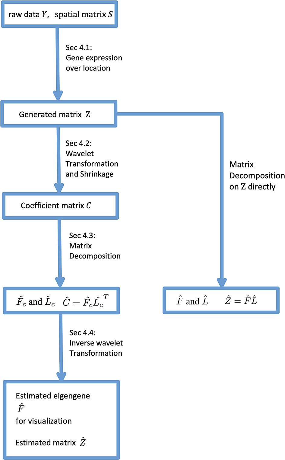
Figure 1. A summary of the proposed workflow.

$\hat{C}$ and $\hat{Z}$ are the estimators for C and Z. F and L are the factor matrix and loading matrix construct as Z = FL, F_c and L_c are the factor matrix and loading matrix construct as C = F_cL_c. $\hat{F}$ and $\hat{F_{c}}$ are the estimators for F and F_c, similiar for Z and $\hat{Z}$ . We will specify the details in Section Background and Problem Setup.

Background

In this section, we will cover background of methods we used in data pre-processing and analysis.

Wavelet transformation

Density estimation and function approximation is a fundamental problem in statistics and machine learning. Non-parametric methods such as spline regression (Perperoglou et al., 2019), Fourier transformation (Cochran et al., 1967) and Wavelet transformation (Nason, 2008) have been used in such scenarios.

Consider a model with one predictor: y = f(x) + ϵ, where ${E ϵ}^{2} = σ^{2}$ . We want to estimate f, the trend of the function. We assume the predictors are ordered x₁ < x₂ < … < x_n. We have a signal or frequency to estimate.

Consider the Haar mother wavelet:

ψ (x) = \{\begin{array}{c} 1 & x \in [0, \frac{1}{2}) \\ - 1 & x \in [\frac{1}{2}, 1) \\ 0 & otherwise \end{array}

satisfying

\int_{- \infty}^{\infty} ψ (x) dx = 0

. Unlike the Fourier basis, wavelets oscillate and decay fast, only contributing to a certain local area and zero elsewhere. We can generate wavelets from the Haar mother wavelet

ψ_{j, k} (x) = 2^{j / 2} ψ (2^{j} x - k)

for integer j, k. These wavelets form orthonormal sets. We can decompose the trend as

f (x) = \sum_{j = - \infty}^{\infty} \sum_{k = - \infty}^{\infty} d_{j, k} ψ_{j, k} (x)

, where

d_{j, k} = \int_{- \infty}^{\infty} f (x) ψ_{j, k} (x) dx = < f, ψ_{j, k} >

are the wavelet coefficients.

Wavelet based methods have several advantages among other non-parametric methods, especially dealing with sparse data. One property wavelet has is localization. If a sequence has a discontinuity, this will only influence the wavelet basis around it. In contrast, for a Fourier basis consisting of sine and cosine functions at different frequencies, every basis element will interact with this discontinuity, hence influencing every Fourier coefficient.

The simplest discrete wavelet transformation calculates the difference and sums between each adjacent pair. Suppose we have one vector with length n, where n is dyadic (n = 2^J). We computed d_{J−1, k} = y_2k − y_2k−1 as finest-level detail and c_{J−1, k} = y_2k + y_2k−1 as the finest-level averages. We have $\{d_{k}\}$ containing n/2 = 2^J−1 as our finest level coefficients. To obtain the next coarsest coeffients we set:

(1)

d_{J - 2, ℓ} = c_{J - 1, 2 ℓ} - c_{J - 1, 2 ℓ - 1}

(2)

\begin{array}{l} c_{J - 2, ℓ} \end{array} = c_{J - 1, 2 ℓ} + c_{J - 1, 2 ℓ - 1}

We continue this procedure until j reaches one. The set of details $\{d_{k}\}$ across levels are our wavelet coefficients.

We use J to denote the scale of wavelets, with larger J we have finer scale and approximation. However, finer scale sometimes introduces more parameters to capture minor details of the sequence (overfitting). The trade-off in choosing J is crucial in the wavelet transformation.

Regularization and smoothing can be used to prevent overfitting. Regularization is usually conducted by shrinking wavelet coefficients. The concept of wavelet shrinkage was first proposed by Donoho and Johnstone (1994). The motivation behind wavelet shrinkage is straightforward. Consider empirical wavelet coefficients, the large coefficients usually contain true signal and noise, whereas the small coefficients only contain noise. The shrinkage is often used when the wavelet coefficients are assumed to be a sparse vector.

Wavelet shrinkage is often conducted by setting a threshold (denoted by δ) and only keeping the coefficients above the threshold. To choose a threshold, a natural metric is the squared error between estimated function and the truth: $\hat{M} = \sum_{i = 1}^{n} {(f (x_{i}) - \hat{f} (x_{i}))}^{2}$ and $M = E \hat{M}$ . Donoho et al. (1994) proposed a universal threshold $δ = σ \sqrt{2 log n}$ , which induced $M \leq O (log n σ^{2})$ . Donoho and Johnstone (1995) also proposed Stein’s unbiased risk estimation (SURE) threshold based on Stein’s (1981) unbiased risk estimator. The optimal SURE threshold can be obtained in $O (n log n)$ operations. Donoho and Johnstone (1995) also noted that SURE sometimes failed when the true signal coefficients are highly sparse, they proposed a hybrid scheme called SureShrink, combining the SURE and universal thresholds, using them depending on certain situations.

The extension of wavelet methods to 2D regularly spaced data (images) and such data in higher dimensions was proposed by Mallat (1989). We only consider 2-D wavelet transformation since we decompose 2-D spatial gene expression data. Suppose we have n × n matrix A where n = 2^J is dyadic. A simple discrete wavelet transformation on A first applies procedure (1) and (2) to the rows of the matrix. We then have two matrices of size $n \times \frac{n}{2}$ , called H and G. Then we apply the same procedures to both the columns of H and G, resulting in four matrices HH, GH, HG, and GG each of size $\frac{n}{2} \times \frac{n}{2}$ . These are our finest level coefficients. HH is the local average of the original matrix used for the next level procedure.

Factor genes

Clustering and dimensionality reduction are widely used in genomics. In a gene-by-sample matrix, genes are often grouped into profiles, where genes from the same profile have a similar function. Statistically, we can treat them as correlated variables. We use the term factor genes as the principal component in our gene-by-sample data. Factor genes compose the linear combinations of genes. We consider each gene as a variable, and we aim to find variables (f₁, …, f_K) such that each gene g_i has form g_i = a₁f₁ + a₂f₂ + ⋯a_Kf_K, where a_j are coefficients.

Suppose we have gene(P)-by-sample(N) matrix $A \in ℝ^{N \times P}$ with sample covariance matrix $S = \frac{1}{n} Ã^{T} Ã$ , where Ã is the column centered A. Consider the SVD on Ã = UΛV^T. Then we have SV = VΛ². The columns of V are called eigenarrays (Alter et al., 2000). The first K columns of Z = AV are the factor genes. The factor genes capture the mutual underlying information of genes.

Empirical Bayes matrix factorization (EBMF)

Matrix Factorization is often used in capture factor genes. We have a formulation similar to Wang and Stephens (2021), consider the factorization model on observed samples by gene data $Y \in ℝ^{N \times P}$

Y = {FL}^{T} + E

where

F \in ℝ^{N \times K}

denotes the factors,

L \in ℝ^{P \times K}

denotes the loadings for each factor, and

E \in ℝ^{N \times P}

denotes Gaussian noise with zero mean. Typical formulations would treat factors and loadings as fixed effects and use Maximum Likelihood Estimation (MLE). In our high-dimensional setting, penalty-based regularizers are often considered. Considering a prior for L and F under Bayesian setting has a similar effect and several advantages over adding a regularizer alone, such as simplifying hyperparameter search and selection of the number of factors K.

One feature of empirical Bayes approaches in matrix factorization proposed by Bishop (1999) is that the methods automatically select the number of factors K. In Wang and Stephens (2021), the author add factors with prior one at a time, estimating priors at each step until convergence. If the computed prior of the newly added factor is almost point mass on 0, the algorithm eliminates this factor and returns.

Following Wang and Stephens (2021), we consider Empirical Bayes in our setting, where we set a prior with unknown parameters of L and F. Empirical Bayes is not strictly Bayes, since the prior parameters are directly estimated by the MLE of the data. One example would be normal distribution $D_{F}$ of F and $D_{L}$ of L where coordinates are independent, which is conjugate prior. We estimate parameters in $D_{F}$ and $D_{L}$ by the maximize the marginal likelihood calculated by integral out L and F. Then we computed the posterior distribution of L and F.

Problem setup

Consider $Y \in ℝ^{N \times P}$ , where each row represents a sample and each column represents a gene. Further, let $S \in ℝ^{N \times 2}$ store spatial coordinates of each sample. We assume there are spatially-related genes among all genes. We assume the genes fall into several profiles. The genes in the same profile have the same expression over the sampled spatial context. For each profile, we can summarize the gene expression for such group by one representative factor. Consider there are K profiles, we can then form our model as:

\begin{array}{l} Y & = \sum_{k = 1}^{K} f_{k} l_{k}^{T} + E \\ = {FL}^{T} + E \end{array}

where

f_{k} \in ℝ^{n}

is the factor gene in profile k capturing the gene expression pattern in that group,

l_{k} \in ℝ^{p}

indicates the loading coefficients of each factor. We assume there is random noise

E \in ℝ^{n \times p}

in observations and

E_{ij} \overset{iid}{\sim} N (0, 1 / τ)

. The goal is to select spatially-related genes based on spatial information in S. We also extract the gene factors which capture information across all genes based on feature extraction. We aim to find a latent gene space that respects spatial structure.

Methods

In this section, we build up pipelines and models to achieve gene dimentionality reduction while retaining spatial structure. We adapt matrix decomposition methods to incorporate spatial information. R is a statistical programming language and will be used for the analysis. We first preprocess gene expression to make them amenable for wavelet filtering. We then use the Daubechies D4 Wavelet Transform (Daubechies, 1992) as wavelet filter with scale of wavelet J = 5. We develop the package and share the workflow generating reproducible quantitative results and gene visualization. The package is available from Software availability.

Gene expression over location

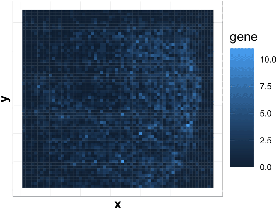
We leverage a pre-processing step, which we call input generation, to combine spatial and expression data. We have both gene expression measurements and spatial coordinates for each sample. Each gene has an expression over each sample, and we can draw the sample over a 2D map by their coordinates.

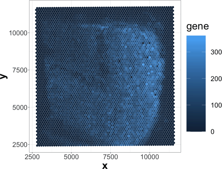
As shown in Figure 2, the gene with the least sparsity in expression shows varying levels of expression across different spatial regions. Intuitively, we may consider the spatial expression pattern from this gene to be spatially related. However, most genes are sparse and do not show fluctuations in gene expression. Therefore, we first filter out those genes using a kOverA filter: we only keep genes that have an expression measure above A in at least k samples (Gentleman et al., 2021). This has the effect of removing genes that are rarely active, though it is possible that strongly expressed genes still show no spatial relationships.

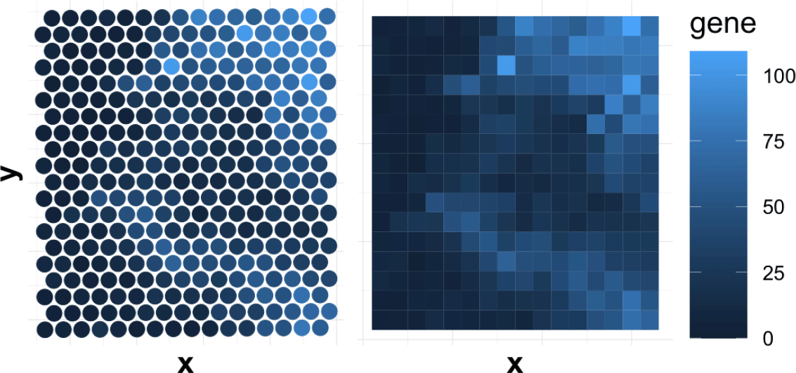
Figure 2. The most dense gene has a structured expression pattern (authors own visualization using ggplot2 package in R).

We want gene expression data to have a neat grid structure that can be expressed as a matrix form. However, at first, expression measurements are roughly staggered over the spatial locations, as shown in Figure 3. This is a consequence of the sampling strategy adopted by the 10x genomics Visium platform. To obtain an evenly resampled version of the expression pattern, we divide the two-dimensional space into several partitions and compute the local average of each partition. Detailes are shown in Algorithm 1. Each gene has an expression over the grid and we now can use a matrix $Z \in ℝ^{D^{2} \times P}$ to represent it. The matrix Z becomes the new input for analysis. We then obtain the same formulation as in Section Problem Setup, where we take n = D² and each location corresponds to a new observation. We have $f_{k} \in ℝ^{D^{2}}, k = 1, \dots, K$ as the factor genes, computed by vectorizing the gene expression matrix.

Figure 3. Left: The gene expression over scattered samples over locations. Right: The local average of gene expression over grid locations, used as input to our algorithms (authors own visualization using ggplot2 package in R).

The choice of D depends on the wavelet scale used in the next section. We choose D to be dyadic to prevent handling edge cases in the wavelet transformation (recalling Subsection Wavelet Transformation). The dyadic size is also a natural choice in image analysis. In particular, we choose D = 2^J, where J is the level of scale in the wavelet transformation. Larger J allows finer recovery, but also requires more parameters and may result in overfitting.

Wavelet transformation and shrinkage

We apply a wavelet transformation with shrinkage to denoise the gene expression matrix and smooth observed spatial expression patterns. In simulations, we find that this technique gives more accurate recovery as the signal-to-noise ratio decreases and yields less noisy visualizations for the spatially-related genes.

We implement wavelet transformation and shrinkage on the processed data matrix $Z \in ℝ^{D^{2} \times P}$ . Each column of Z is a vectorized expression matrix. For each column, we first reshape it into a D × D matrix and apply the wavelet transformation. We have a coefficient list with W coefficients associated with each gene. Then we conduct wavelet shrinkage on the coefficient list using the threshold strategies described in Subsection Wavelet Transformation. Finally, we vectorize the coefficient list of each gene into a length W vector for each gene. Stacking all vectors together, we have a coefficient matrix $C \in ℝ^{W \times P}$ . Note that the wavelet scale is specified by the size D of the input matrix, i.e., we have D = 2^J, where J is the scale. The details are specified in Algorithm 2.

Matrix decomposition

The matrix of the shrunk wavelet coefficients C gives a summary of the denoised matrix. This allows improved reconstruction of gene expression data. To obtain a low-dimensional approximation, we apply matrix factorization on the coefficient matrix C after transformation. We use the same notation in Section Problem Setup, with the subscript c to denote the decomposition on coefficient matrix C.

The resulting singular vectors can be used to estimate spatially structured factor genes (Subsection Factor Gene). We use SVD as a frequentist approach to estimating $\hat{F_{c}}$ and ${\hat{L}}_{c}$ . We also conduct EBMF (Section Empirical Bayes Matrix Factorization), using the posterior expectation of F_c and L_c to estimate $\hat{F_{c}}$ and $\hat{L_{c}}$ . EBMF can select the number of factors K by itself, whereas K must be manually specified in the SVD. The choice of K is informed by inspecting the scree plot, as in spectral clustering and PCA. We choose the number of factors when current factors explain sufficient information and the diminishing returns of additional factors are no longer worth the additional cost. Given ${\hat{F}}_{c}$ and ${\hat{L}}_{C}$ , we can compute the estimated coefficient matrix as $\hat{C} = {\hat{F}}_{c} {\hat{L}}_{c}^{T}$ .

Inverse wavelet transformation

To transfer the coefficient matrix $\hat{C}$ back to the estimated location-by-gene matrix $\hat{Z}$ , we apply the inverse wavelet transformation on columns of $\hat{C}$ , each of which is a vectorized coefficient list for one gene. This results in a D² expression matrix for each gene. Then we vectorize the matrix and stack all vectors together. This yields the reconstructed matrix $\hat{Z}$ . Details are given in Algorithm 3. For visualization, we also conduct a similar process for each column of $\hat{F_{c}}$ . In this case, each column is associated with an factor gene. By applying the inverse wavelet transformation to each factor gene, we can build spatial gene expression matrices M₁, …, M_K representing gene factors.

Alogorithm 1. Input generation.

Require Sample by gene matrix $Y \in ℝ^{N \times P}$ , spatial matrix $S \in ℝ^{N \times 2}$ , size of gene expression matrix D

1: Compute the range of x, y coordinates from S, compute the coordinates of vertices of big rectangle map B cover all N samples spatially.

2: Partition interval x and interval y into D equal length interval, together get D² partitions over rectangle B.

3: while i ≤ P do ⊳ Consider gene i expression over map B

4: Select i-th column of gene matrix Y

5: Compute the local average of gene expression of gene i in each partition

6: Get D² matrix G_i as gene expression of gene i

7: Vectorize G_i into a vector g_i with length D²

8: end while

9: Stacking all ${\{g_{i}\}}_{i = l}^{P}$ together into matrix $Z \in ℝ^{D^{2} \times P}$

10: return matrix Z ⊳ A transformed gene expression matrix

Algorithm 2. Wavelet transformation and shrinkage.

Require Location by gene matrix $Z \in ℝ^{D^{2} \times P}$ , threshold method, optional threshold parameter τ. ⊳ Apply threshold on wavelet coefficient if threshold method is specified

1: while i ≤ P do ⊳ Consider gene i expression as matrix G_i

2: Select i^th g_i column of gene matrix Z

3: Form g_i into expression matrix G_i with size D²

4: Apply 2-D discrete wavelet transformation over G_i, get coefficient list C_i, with number of coefficients W

5: Apply wavelet shrinkage over C_i with optional parameter τ

6: Vectorize C_i into a long vector c_i with length W

7: end while

8: Stacking all ${\{c_{i}\}}_{i = l}^{P}$ together into matrix $C \in ℝ^{W \times P}$

9: return coefficient matrix C ⊳ Column i of C store the coefficient of from gene i

Algorithm 3. Inverse wavelet transformation.

Require: (reconstructed) Coefficient matrix C

1: while i ≤ P do

2: Select i^th c_i column of gene matrix C

3: Form c_i into coefficient list C_i with number of coefficients W

4: Apply 2-D inverse wavelet transformation over C_i, get post-wavelet expression matrix $\hat{G_{i}}$

5: Vectorize $\hat{G_{i}}$ into a long vector $\hat{g_{i}}$ with length D²

6: end while

7: Stacking all ${\{\hat{g_{i}}\}}_{i = 1}^{P}$ together into matrix $\hat{Z} \in ℝ^{D^{2} \times P}$

8: return matrix $\hat{Z}$ ⊳ Post processing reconstructed gene expression matrix

Evaluation

We evaluate our proposal both quantitatively and qualitatively. Our quantitative results measures reconstruction error between the estimated $\hat{Z}$ and Z using the Frobenius norm ${‖\hat{Z} - Z‖}_{F}^{2}$ .

This evaluation is also used for hyperparameter tuning, such as the scale J of the wavelet and the choice of wavelet thresholding method. Our qualitative result is given by visualization of the estimated factor gene expression matrices, with emphasis on capturing global spatial structure.

We use cross-validation in computing reconstruction error and calculating gene-wise errors. This evaluation is helpful in selecting spatially related genes. We also found a simple connection between the gradient of gene expression and spatial contribution, discussed in Section Real Data Experiment. This discussion requires a measure of spatial expression smoothness. To this end, a simple step computing the fluctuation of gene expression would give a spatial gene selection that coincides with the reconstruction error selection. For calculating successive differences, consider Z as the input matrix and let δ_jk = (z_{j, k+1}−z_jk)², k = 1, …, D². Then we define the gradient by $\sum_{jk} δ_{jk}$ .

Simulation

We setup simulations to see whether representing spatial structure with a wavelet basis supports denoising and visualization of gene expression. We will see improved recovery in the low signal-to-noise ratio regime. Qualitatively, we also find factor gene visualizations to be more spatially consistent. We use use the Daubechies D4 Wavelet Transform (Daubechies, 1992) as wavelet filter with scale of wavelet J = 5. We develop the package and share the workflow generating reproducible quantitative results and gene visualization. The package is available from Software availability.

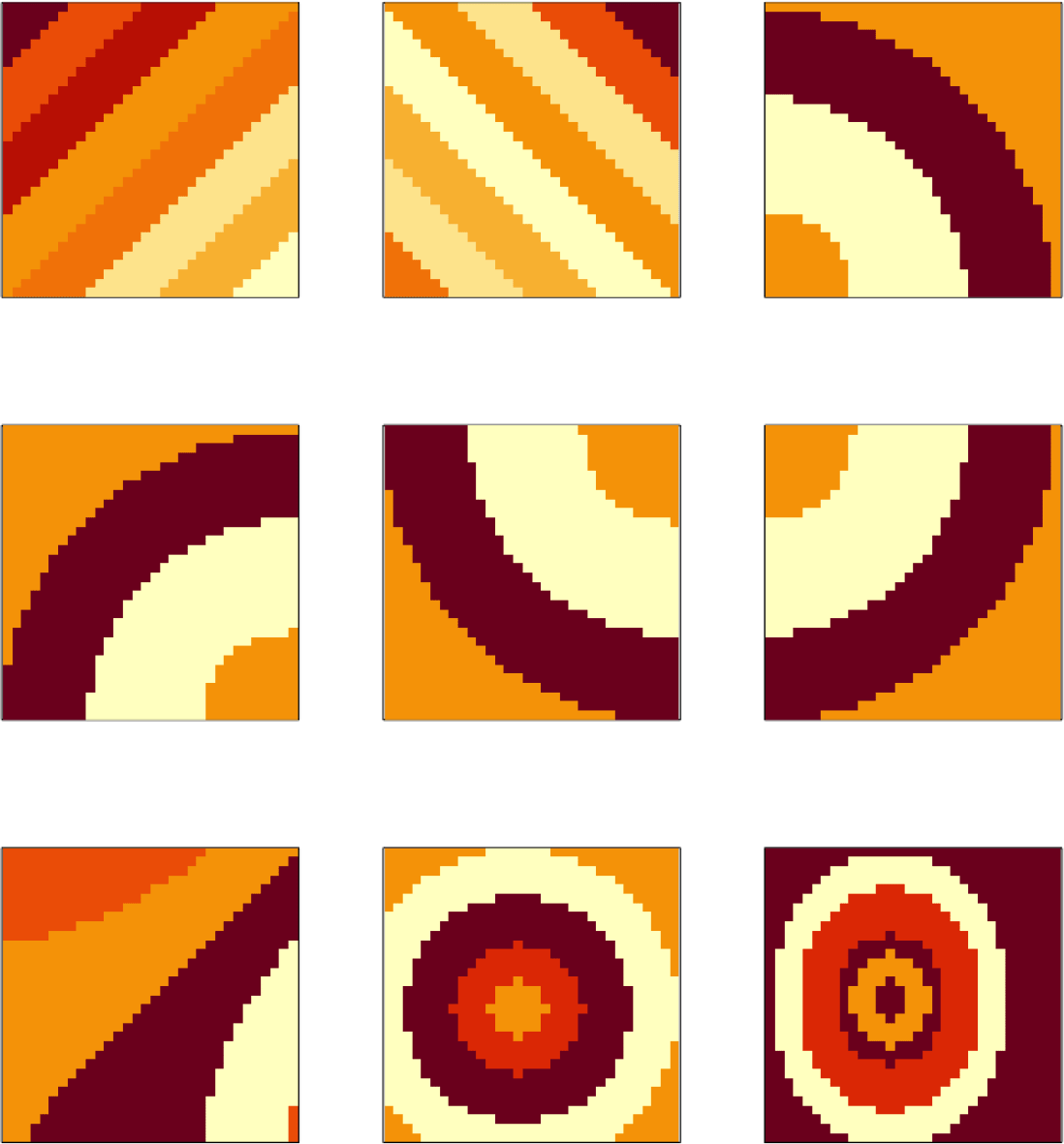
We first describe the simulation mechanism. We the set number of factors to K = 9. We generate K gene expression matrices $M_{1}, \dots, M_{K} \in ℝ^{D^{2}}$ , each representing a factor gene. These factor gene expression patterns are shown in Figure 4. We vectorize the patterns M_k into factor genes f_k, which are then scaled so ∥f_k∥ = 1. We obtain $F \in ℝ^{D^{2} \times K}$ by stacking all the f_k together. We generate loadings $l_{1}, \dots, l_{K} \in ℝ^{P \times K}$ by drawing coordinates independently from N(0, 1). We set D = 32 and wavelet scale J = 5. We similarly stack l_k to obtain $L \in ℝ^{P \times K}$ . We use Z = FL^T as the ground-truth signal matrix and add noise E to yield data matrix Z_d = FL^T + E, where entries in E are zero-mean normal noise that corrupt the underlying signal. In our analysis, we use a Daubechies D4 Wavelet as the wavelet filter, and for coefficient shrinkage we use hybrid thresholding.

Figure 4. The gene expression pattern for nine factor genes in the simulation experiment (authors own visualization using ggplot2 package in R).

We use the pipeline from Section Methods. The generated data Z_d already reflects the structure produced by the processing of Subsection Gene Expression Over Location. For comparison, we also directly decompose the matrix Z_d with the SVD without any wavelet transformation. We call the resulting factors ${\hat{F}}_{raw}$ and reconstruction ${\hat{Z}}_{raw}$ . We also have the same quantitative reconstruction error and qualitative visualization of factor gene ${\hat{F}}_{raw}$ . We also measure the size of the gradients across the estimated gene expression matrix ${\hat{M}}_{i}$ . The gradient is computed by successive difference of neighboring image pixels. We calculated the sum of the squares of the gradient. This measurement shows whether the gene expression matrix has been smoothed. This property is of interest, since smoother estimates are often more visually appealing.

We denote the signal-to-noise ratio as $SNR = \frac{sd (Z)}{sd (E)}$ , where sd stands for standard deviation. Let $r = \frac{1}{SNR}$ . We specify 19 evenly spaced settings of r from 1 to 10. For each setting, we run 100 replicates with different simulated Z_d and apply wavelet and SVD-based dimensionality reduction. The resulting average errors across r are shown in the Figure 5. The wavelet and shrinkage technique has better performance when r is larger than 5, i.e., the low signal-to-noise ratio regime. The gradient of the gene expression matrix under two methods is shown in Figure 5. The wavelet and shrinkage approach smooths edges in the factor gene expression image, giving a more interpretable visualization and lower error in this low SNR setting.

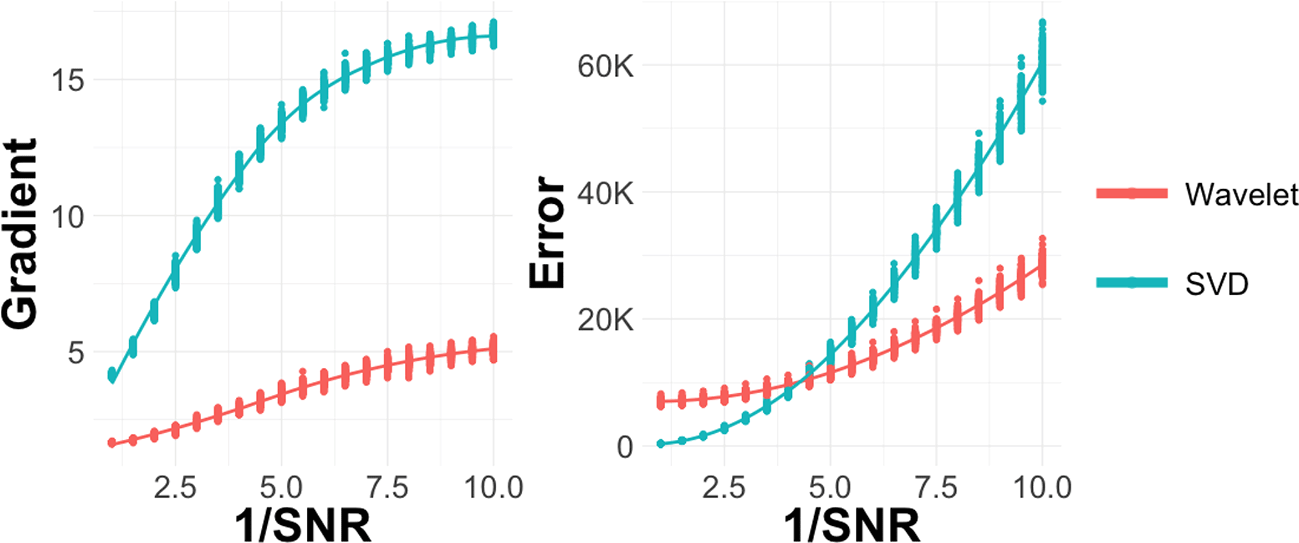
Figure 5. The reconstruction error and gradient for estimated gene-by-location matrix with different SNR (signal-to-noise regime).

The x-axis shows the rate of $\frac{1}{SNR}$ The left subplot shows the gradient changes. The gradient of gene expression is always lower with the wavelet technique, a consequence of its smoothing property. The right subplot shows the error – the wavelet method has lower error as the magnitude of noise increase. The underlying data can be found as simulation_data in package from Software availability. SVD, singular value decomposition.

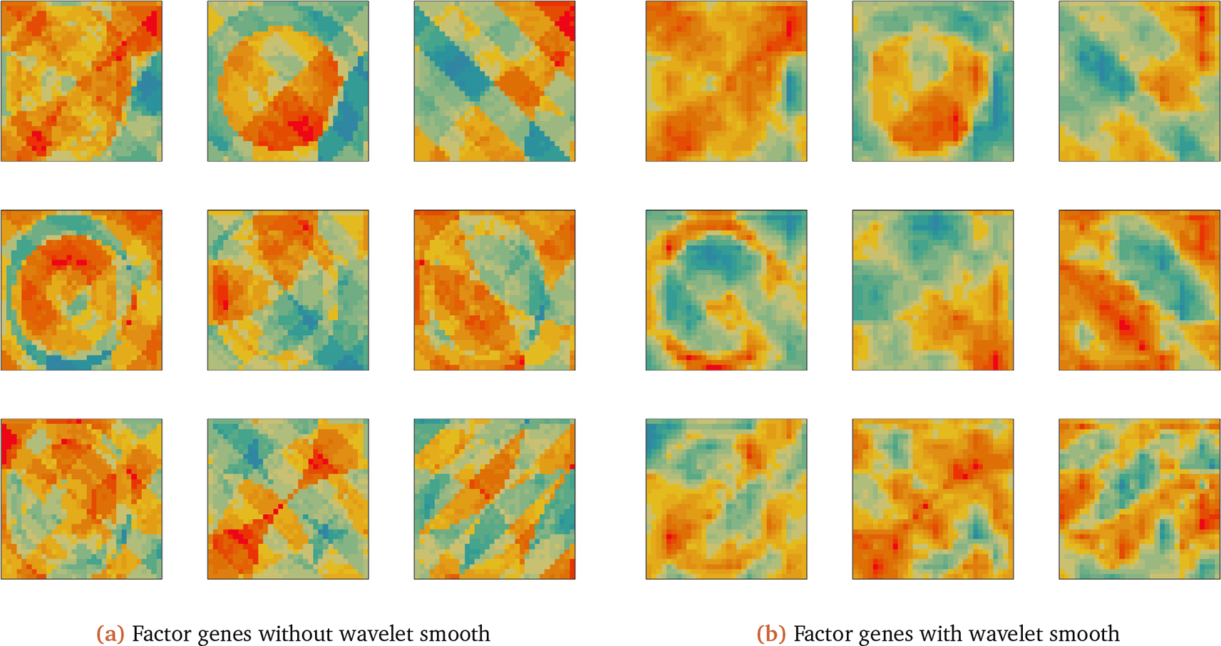
The factor genes are shown in Figure 6. The SVD without wavelet technique has erratic, outlying pixels, especially in the last three genes. The visualization is sensitive to outliers. In contrast, the SVD combined with wavelet has smoother patterns. Like the SVD-based method, it appears to have mixed several of the true underlying factors in each of the recovered ones. Moreover, the sharp boundaries visible in the SVD factors become smoothed over in the wavelet-decomposition. The wavelet method applies a decomposition on coefficients space after thresholding, while SVD operates on individual pixels. The SVD capture more information, but also emphasize nuisance information induced by errors. Wavelet method also reduces model complexity, improving estimation accuracy. Other non-parametric methods, such as Fourier transformation and Gaussian Process-based methods also operate on coefficients space. Still, they would struggle to capture sharp transitions, since their bases are smooth functions.

Figure 6. Factor gene visualization.

(a) Implements SVD on Z_d, the visualization of column of ${\hat{F}}_{raw}$ . (b) Implements SVD on coefficient matrix, the visualization of $\hat{F}$ . We use Z = FL^T as the ground-truth signal matrix and add noise E to yield data matrix Z_d = FL^T + E, where entries in E are zero-mean normal noise that corrupt the underlying signal. For comparison, we also directly decompose the matrix Z_d with the SVD without any wavelet transformation. We call the resulting factors ${\hat{F}}_{raw}$ and reconstruction ${\hat{Z}}_{raw}$ . We also have the same quantitative reconstruction error and qualitative visualization of factor gene ${\hat{F}}_{raw}$ . (authors own visualization using ggplot2 package in R).

Nonetheless, both the SVD and wavelet-based visualizations reflect spatial trends in the true factor genes (in Figure 4).

Real data experiment

In this section, we show that wavelet and shrinkage technique reduces reconstruction error quantitatively. We ran our method on a public spatially resolved transcriptomics data (Weber, 2021). The dataset can be accessed in R package STexampleData with version 3.15. The dataset represents a single biological sample from the human brain dorsolateral prefrontal cortex (DLPFC) region, measured with the 10x Genomics Visium platform. Further, we identify a simple connection between the gradient of gene expression and quantitative error. A simple step computing the fluctuation of gene expression alone (calculating successive difference of the gene expression image) selects genes that have reduced reconstruction error when using wavelet-guided dimensionality reduction (Zhuoyan, 2022).

We first process the ST data through our pipeline. The ST data contains 4992 observations with 33538 genes. Expressions from most genes are sparse. We implement the pipeline from Section Methods. We pre-process as in Subsection Gene Expression Over Location and then apply a kOverA filter to select genes. We find k = 3, A = 7 gives us 721 genes with average expression as 2.71. Then we apply Algorithm 1 to transfer the sample-by-gene matrix to a grid-by-gene matrix. We set D = 64 and wavelet scale J = 6. We obtain an image heatmap for each gene like in Figure 7.

Figure 7. Gene expression over the grid (authors own visualization using ggplot2 package in R).

We then vectorize P = 721 image expression and stacking vectors together, we have generated input data $Z \in ℝ^{64^{2} \times 721}$ . We run our pipelines with and without wavelet transformation for evaluation. We first implement SVD and EBMF on Z or on coefficient matrix C after applying wavelet transformation and thresholding each column. We choose the number of factors K by examining singular values. If the singular value is larger than 500, we keep it as a factor. In EBMF, we set upper bound that K to be smaller than the corresponding K in SVD, then let algorithm choose K itself.

Quantitative evaluation metric is conducted by cross-validation on non-zero entries. We set 5 folds cross-validation with replacement. In particular, we select random $\frac{1}{5}$ non-zero entries in matrix Z and set them to zero, then we save matrix as the masked matrix (train data) Z_train. We store the values and position of the masked entries as test data Z_test. We then ran methods on Z_train. The result shows a difference in whether to use the wavelet technique. The result from SVD and EBMF are close to each other coordinate-wise, hence we only show one of them in some results below. We include the comparison between SVD and EBMF in the Section Comparison between SVD and EBMF. As in Section Simulation, we have $\hat{F}$ and $\hat{Z}$ from the wavelet approach and ${\hat{F}}_{raw}$ and ${\hat{Z}}_{raw}$ on the original data.

Total error and parameter tuning

We compute the reconstruction loss,

\frac{1}{N} \sum_{i, j \in test} {({\hat{Z}}_{ij} - Z_{ij})}^{2}

where N is the number of test entries. We evaluate the loss only on test entries. We first tune parameters. We set up three settings: decompose the raw data with SVD or EBMF; wavelet transformation with hybrid thresholding; wavelet transformation with manual thresholding with threshold τ = 10, 20, …, 100. In each setting, we ran 100 replicates. The reconstruction error shown in Figure 8.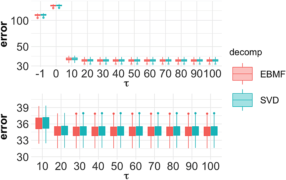

Figure 8. The reconstruction error for different wavelet parameters.

The upper plot contains the result from all settings, the leftmost τ = −1 result is the decomposition without wavelet transformation. τ = 0 indicates the hybrid thresholding. The bottom plot zooms into the experiment under manual threshold for $τ \in [10, 100]$ . SVD, singular value decomposition; EBMF, Empirical Bayes Matrix Factorization.

As shown in the upper panel of Figure 8, wavelet thresholding with manually set τ reduces error compared to decomposing raw data. The wavelet has the most positive effect when τ = 40, as shown in the bottom panel. We use τ = 40 in our following analysis.

Genewise error

We then evaluate how method performance varies for each gene by calculating the genewise reconstruction error. This reveals genes whose strong spatial expression structure leads to improved performance when using a wavelet basis. We still hold out $\frac{1}{5}$ of the entries at random as a test set. We compute the reconstruction error of test entries on each column of $\hat{Z} - Z$ . We calculate entry-wise loss across 100 replicates and estimate the average loss. We compare genewise errors with or without wavelet transformation. The SVD and EBMF show the same result regarding the decomposition method. We only show result of EBMF here in Figure 9. We show the result of SVD in Figure 13b.

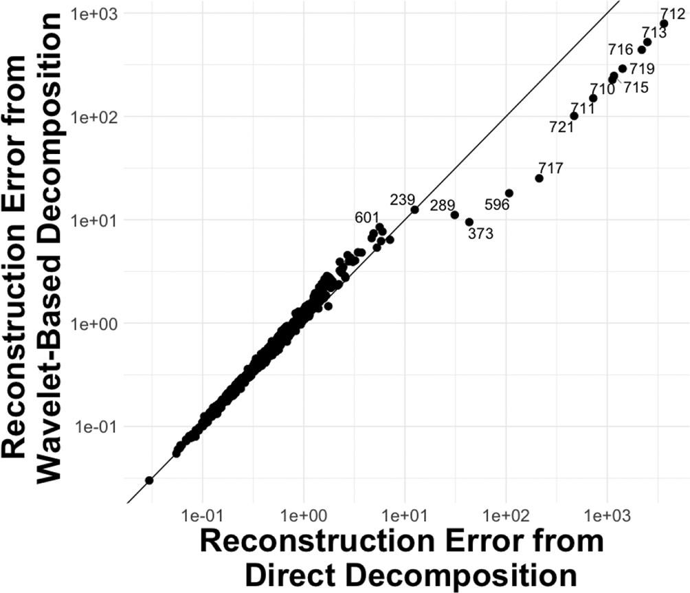
Figure 9. The reconstruction error for each gene. The x-axis is the error from EBMF on raw data, the y-axis is the error from the combination of wavelet thresholding and EBMF.

As we can see, most of the genes have lower reconstruction error when directly applying the SVD or EBMF. However, for some genes, wavelet smoothing reduces error. For example, this is seen in genes 712, 713, 716, 719, 715, 710, 711, 721, 717, 596, 373, and 289. We conjecture that these genes have acute fluctuations as well as clear spatial patterns. The expression matrix of these genes would have a larger gradient and distinct edges. To verify our conjecture, we calculated the sum of squares of the gradient of each gene expression matrix. We show the result in Figure 10.

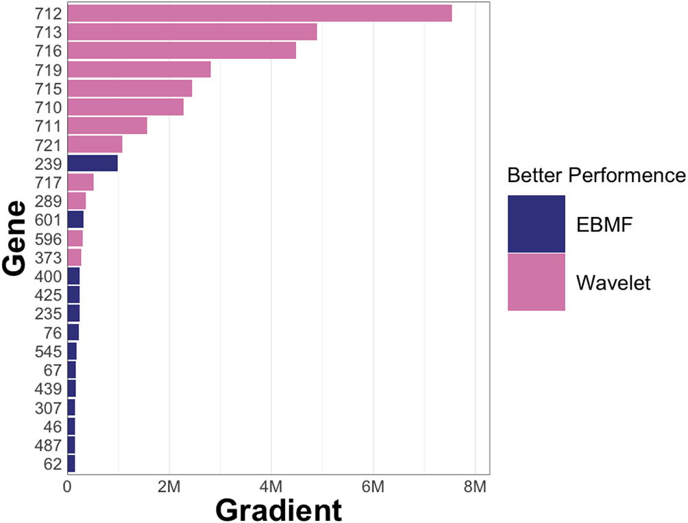
Figure 10. The sum of squares of the gradient for each gene.

The y-axis is the index of each gene. Each bar’s color shows whether that gene has better performance when using a wavelet basis. The M on the x-axis stands for “millions”. EBMF, Empirical Bayes Matrix Factorization.

The result verifies our conjecture: genes with larger gradients have better reconstruction under the wavelet-guided decomposition. This suggests a pre-processing step for selecting wavelet-suited genes by calculating the gradient of each gene. The spatially related genes would have a lower reconstruction error. Among these spatially related genes, one possibility is that we can divide them into two groups, one for decomposition directly and the other for the wavelet technique.

Factor genes

Now we visualize the top factor genes and genes with high loadings on these factor genes. In Figure 11a, we decompose Z using the SVD and plot the first factor gene and matrix slides of genes with the largest 5 loadings on that factor. The factor gene captured the same patterns as the original genes. To improve visualization, we find the analogous wavelet-based factors (we use manual thresholding with τ = 40), shown in Figure 11b.

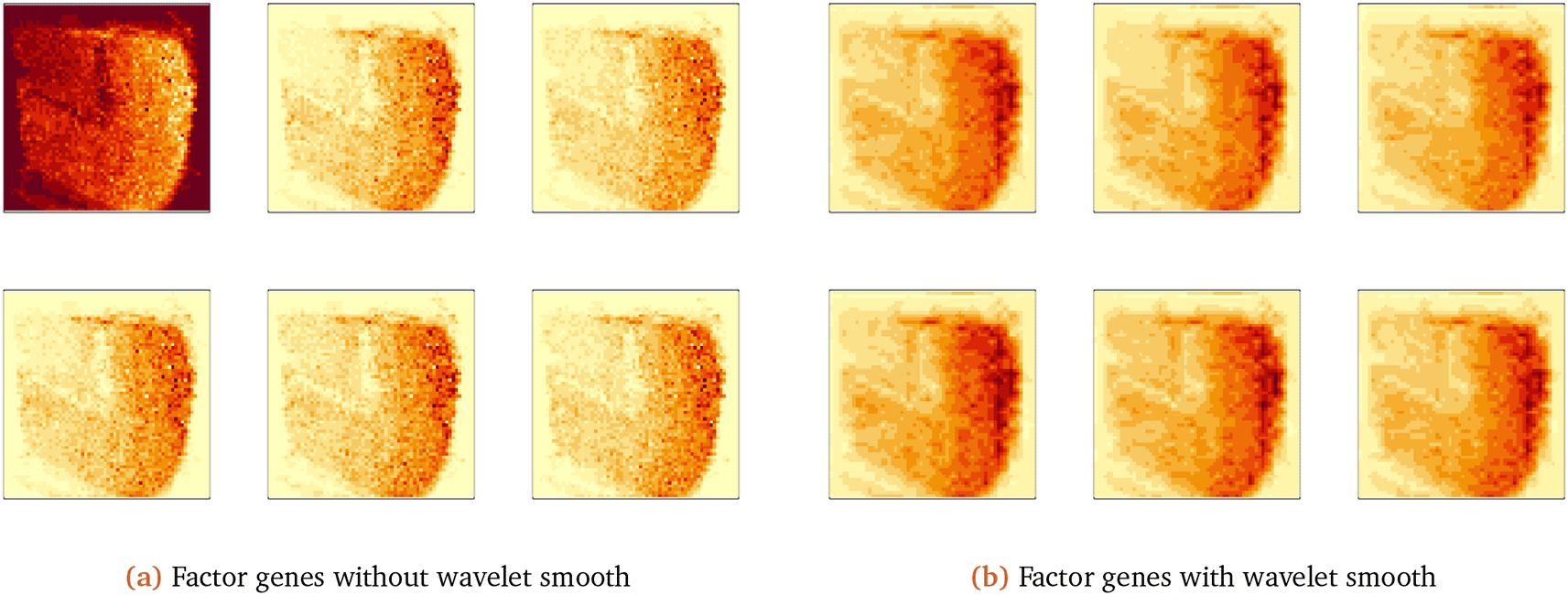
Figure 11. The top left figure is first factor gene, the following figure by row is genes with largest loadings on first factor gene: gene 712, 713, 716, 719, 715 (authors own visualization using ggplot2 package in R).

The wavelet thresholding approach smooths over edges in the original visualization. The first factor gene captures the global spatial expression. We have a similar result for the second factor gene, as shown in Figure 12.

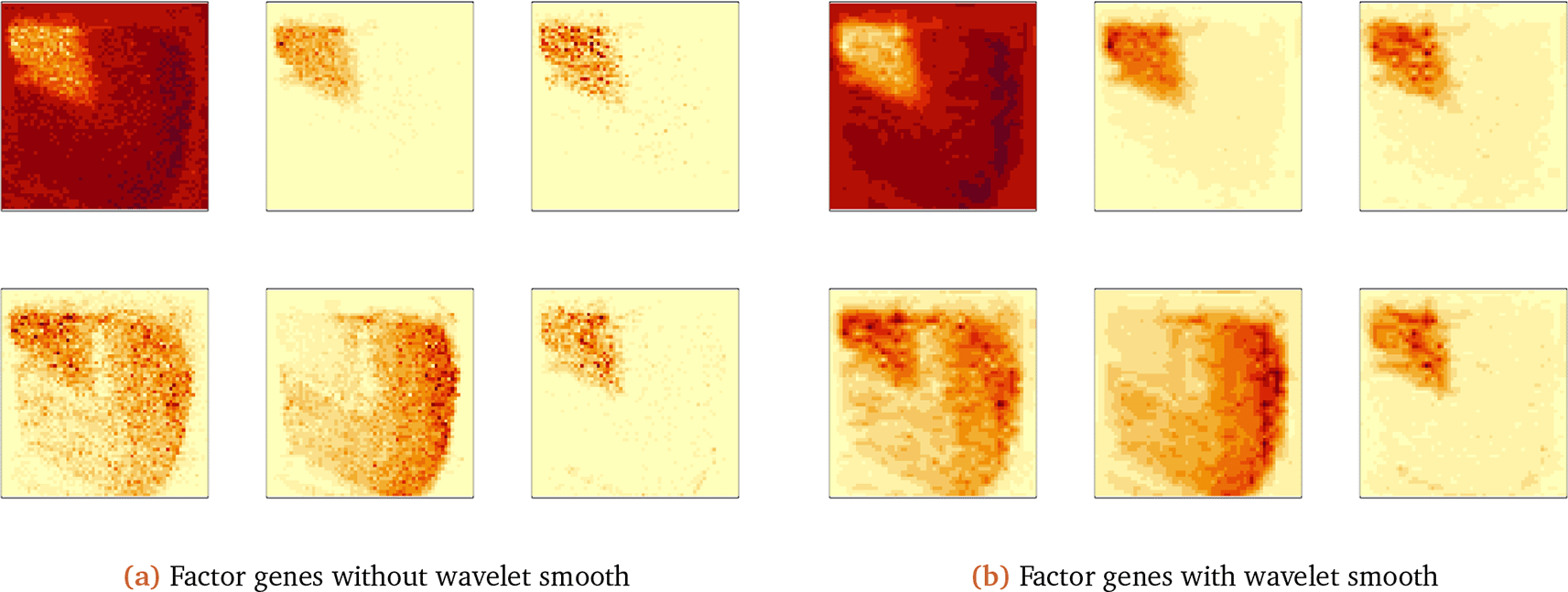
Figure 12. The top left figure is the second factor gene, the following figure by row is genes with largest loadings on second factor gene: gene 596, 289, 373, 712, 578 (authors own visualization using ggplot2 package in R).

The second factor gene is orthogonal to the first one, capturing different spatial structures in gene expression. Different factor genes capture global and local structure, and using a wavelet decomposition provides denoised spatial expression visualization.

In conclusion, we can use this dimensionality reduction technique for spatial gene selection and extraction. We select wavelet-suited genes based on the calculated gradient. Then, we can select spatially related genes based on reconstruction error via cross-validation. Alternatively, we can extract factor gene to capture spatial information and use factor genes for visualization and further analysis.

Software

We provide a small code block to show vignette of generating Figure 11 and Figure 12, shown in code block 1.

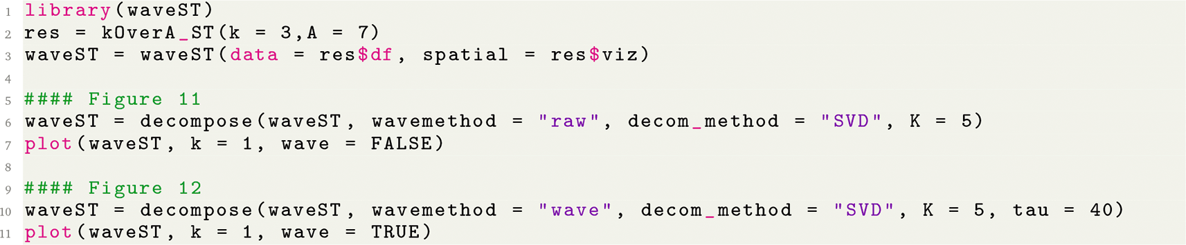
Listing 1. The basic wavelet-based dimensionality reduction workflow.

kOverA_ST transforms the original spatial expression context into an image. This is processed by waveST. The final dimensionality reduction step is performed by decompose.

We have made a new package waveST containing the workflow we developed. The package is available at GitHub (see Software availability). The kOverA_ST function reduces data from an original (Weber, 2021) class input using the kOverA technique. Then we use waveST function to construct a S4 class waveST, containing input generated by Algorithm 1. This object-oriented approach stores properties of the original spatial experiment and simplifies downstream calls, like decomposition and visualization. We use the decompose function to apply all decomposition methods. In line 6, we apply the SVD to our original data, setting the number of factors to 5. In line 11, we apply the wavelet-based reduction and apply a manual threshold with τ = 40. We use plot and k=1 to visualize the first factor gene and matrix slides of the genes with the largest 5 loadings on that factor.

Comparison between SVD and EBMF

This section we provide a comparison between the reconstruction results when using SVD and EBMF. In general, we find little difference between reduction using the two methods. We first provide an element-wise comparison between the reconstruction of SVD and of EBMF with wavelet technique in Figure 13a.

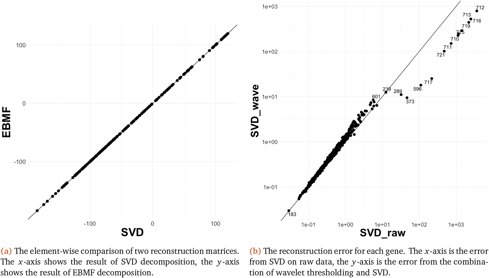
Figure 13. The reconstruction error for each gene.

SVD, singular value decomposition; EBMF, Empirical Bayes Matrix Factorization.

The results are similar when applied to real data. In particular, Figure 13b shows the reconstuction error per gene result for SVD. Our findings are similar to those for Figure 9. Similar findings are visible when using SVD and EBMF with and without an initial wavelet decomposition Figure 14. As we can see, SVD and Empirical Bayes Matrix Factorization (EBMF) have the very similar result. This is perhaps a consequence of EMBF being initialized usign the SVD.

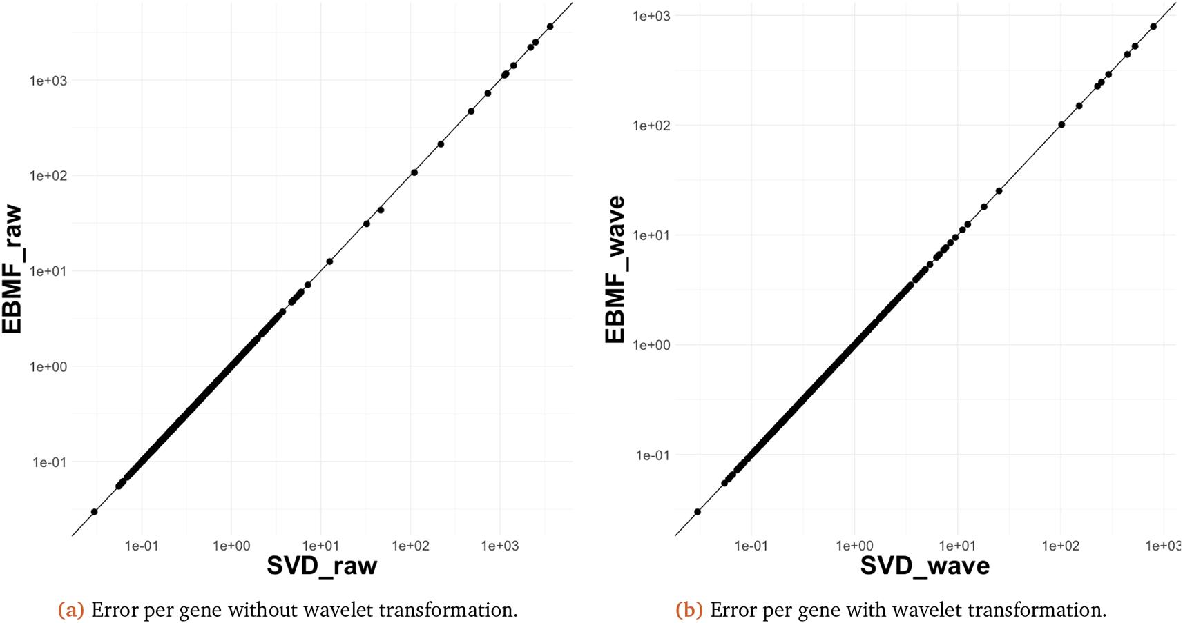
Figure 14. The reconstruction error for each gene.

SVD, singular value decomposition; EBMF, Empirical Bayes Matrix Factorization.

Conclusions

We have proposed a pipeline for dimensionality reduction that respects spatial structure. Both simulations and real data experiments demonstrate that wavelet and shrinkage techniques show positive results in spatially resolved transcriptomics data. We highlight the idea of combining image processing techniques and statistical methods for application in a spatial genomics context. One future direction is splitting genes into a groups suited or not for wavelet-based decomposition, and implementing decomposition with or without wavelet. Another direction is to focus input generation on only those genes that are thought to be spatially related. For genes not related to spatial information, we may perform regular decomposition on original data $Y \in ℝ^{N \times P}$ , abandoning the spatial information of those genes. We expect this to improve reconstruction performance. In further analysis, it is worth considering other wavelet smoothing techniques and wavelet filters. The current methods incorporate little biological information. Bringing more domain knowledge will require further techniques, but is expected to yield better results. The input generation computes local average over even grids; however, it is possible to apply the wavelet method for irregularly spaced data (Nason, 2008). We hope wavelet methods will be useful in adapting existing methods for statistical genomics to the spatial setting.

Data availability

We ran our method on a public spatially resolved transcriptomics data (Weber, 2021). The dataset can be accessed in R package STexampleData with version 3.15. The dataset represents a single biological sample from the human brain dorsolateral prefrontal cortex (DLPFC) region, measured with the 10x Genomics Visium platform. The data used for this study can be accessed though our R package available at Zhuoyan (2022). The data in Simulation is labelled simulation_data and, the data in Real Data Experiment is labelled raws. The data source for generating raws can be accessed though function Visium_humanDLPFC in R package STexampleData with version 3.15.

Underlying data

Zenodo: OliverXUZY/waveST: waveST. https://doi.org/10.5281/zenodo.6983923 (Zhuoyan, 2022)

This project contains the following underlying data:

raws.rda

simulation_data.rda

Data are available under the terms of the Creative Commons Zero “No rights reserved” data waiver (CC0 1.0 Public domain dedication).

Software availability

Source code available from: https://github.com/OliverXUZY/waveST.

Archived source code at time of publication: https://doi.org/10.5281/zenodo.6983923.

License: The software is licensed under MIT

Acknowledgements

We thank Joseph Arthur for valuable discussions.

References

Abu-Jamous B, Kelly S: Clust: automatic extraction of optimal co-expressed gene clusters from gene expression data. Genome Biol. 2018; 19(1): 1–11.
Alter O, Brown PO, Botstein D: Singular value decomposition for genome-wide expression data processing and modeling. Proc. Natl. Acad. Sci. 2000; 97(18): 10101–10106. PubMed Abstract | Publisher Full Text | Free Full Text
Asp M, Giacomello S, Larsson L, et al.: A spatiotemporal organ-wide gene expression and cell atlas of the developing human heart. Cell. 2019; 179(7): 1647–1660.e19. PubMed Abstract | Publisher Full Text
Berglund E, Maaskola J, Schultz N, et al.: Spatial maps of prostate cancer transcriptomes reveal an unexplored landscape of heterogeneity. Nat. Commun. 2018; 9(1): 1–13. Publisher Full Text
Bishop CM: Variational principal components.1999.
Chen KH, Boettiger AN, Moffitt JR, et al.: Spatially resolved, highly multiplexed rna profiling in single cells. Science. 2015; 348(6233): aaa6090. PubMed Abstract | Publisher Full Text
Close JL, Long BR, Zeng H: Spatially resolved transcriptomics in neuroscience. Nat. Methods. 2021; 18(1): 23–25. PubMed Abstract | Publisher Full Text
Cochran WT, Cooley JW, Favin DL, et al.: What is the fast fourier transform? Proc. IEEE. 1967; 55(10): 1664–1674. Publisher Full Text
Daubechies I: Ten lectures on wavelets. SIAM;1992.
Donoho DL, Johnstone JM: Ideal spatial adaptation by wavelet shrinkage. Biometrika. 1994; 81(3): 425–455. Publisher Full Text
Donoho DL, Johnstone IM, et al.: Ideal denoising in an orthonormal basis chosen from a library of bases. Comptes rendus de l’Académie des sciences. Série I, Mathématique. 1994; 319(12): 1317–1322.
Donoho DL, Johnstone IM: Adapting to unknown smoothness via wavelet shrinkage. J. Am. Stat. Assoc. 1995; 90(432): 1200–1224. Publisher Full Text
Dumitrascu B, Villar S, Mixon DG, et al.: Optimal marker gene selection for cell type discrimination in single cell analyses. Nat. Commun. 2021; 12(1): 1–8. Publisher Full Text
Gentleman R, Carey VJ, Huber W, et al.: genefilter: genefilter: methods for filtering genes from high-throughput experiments. 2021. R package version 1.74.0.
Kiselev VY, Kirschner K, Schaub MT, et al.: Sc3 - consensus clustering of single-cell rna-seq data. Nat. Methods. 2017; 14: 483–486. PubMed Abstract | Publisher Full Text
Kiselev VY, Yiu A, Hemberg M: scmap: projection of single-cell rna-seq data across data sets. Nat. Methods. 2018; 15(5): 359–362. PubMed Abstract | Publisher Full Text
Kuppe C, Ramirez Flores RO, Li Z, et al.: Spatial multi-omic map of human myocardial infarction. BioRxiv. 2020.
Mallat SG: A theory for multiresolution signal decomposition: the wavelet representation. IEEE Trans. Pattern Anal. Mach. Intell. 1989; 11(7): 674–693. Publisher Full Text
Moffitt JR, Hao J, Wang G, et al.: High-throughput single-cell gene-expression profiling with multiplexed error-robust fluorescence in situ hybridization. Proc. Natl. Acad. Sci. 2016; 113(39): 11046–11051. PubMed Abstract | Publisher Full Text | Free Full Text
Moncada R, Barkley D, Wagner F, et al.: Integrating microarray-based spatial transcriptomics and single-cell rna-seq reveals tissue architecture in pancreatic ductal adenocarcinomas. Nat. Biotechnol. 2020; 38(3): 333–342. PubMed Abstract | Publisher Full Text
Nason GP: Wavelet methods in statistics with R. Springer;2008.
Perperoglou A, Sauerbrei W, Abrahamowicz M, et al.: A review of spline function procedures in r. BMC Med. Res. Methodol. 2019; 19(1): 1–16. Publisher Full Text
Rodriques SG, Stickels RR, Goeva A, et al.: Slide-seq: A scalable technology for measuring genome-wide expression at high spatial resolution. Science. 2019; 363(6434): 1463–1467. PubMed Abstract | Publisher Full Text
Rödelsperger C, Ebbing A, Sharma DR, et al.: Spatial transcriptomics of nematodes identifies sperm cells as a source of genomic novelty and rapid evolution. Mol. Biol. Evol. 2021; 38(1): 229–243. PubMed Abstract | Publisher Full Text
Shah S, Lubeck E, Zhou W, et al.: In situ transcription profiling of single cells reveals spatial organization of cells in the mouse hippocampus. Neuron. 2016; 92(2): 342–357. PubMed Abstract | Publisher Full Text | Free Full Text
Shang L, Zhou X: Spatially aware dimension reduction for spatial transcriptomics. bioRxiv. 2022.
Srivatsan SR, Regier MC, Barkan E, et al.: Embryo-scale, single-cell spatial transcriptomics. Science. 2021; 373(6550): 111–117. PubMed Abstract | Publisher Full Text
Ståhl PL, Salmén F, Vickovic S, et al.: Visualization and analysis of gene expression in tissue sections by spatial transcriptomics. Science. 2016; 353(6294): 78–82. PubMed Abstract | Publisher Full Text
Svensson V, Teichmann SA, Stegle O: Spatialde: identification of spatially variable genes. Nat. Methods. 2018; 15(5): 343–346. PubMed Abstract | Publisher Full Text
Thrane K, Eriksson H, Maaskola J, et al.: Spatially resolved transcriptomics enables dissection of genetic heterogeneity in stage iii cutaneous malignant melanoma. Cancer Res. 2018; 78(20): 5970–5979. PubMed Abstract | Publisher Full Text
Townes FW, Engelhardt BE: Nonnegative spatial factorization. arXiv preprint arXiv:2110.06122. 2021.
Weber LM: STexampleData: Collection of spatially resolved transcriptomics datasets in SpatialExperiment Bioconductor format. 2021. R package version 1.0.8.Reference Source
Velten B, Braunger JM, Argelaguet R, et al.: Identifying temporal and spatial patterns of variation from multimodal data using mefisto. Nat. Methods. 2022; 19: 179–186. Publisher Full Text
Wang W, Stephens M: Empirical bayes matrix factorization. J. Mach. Learn. Res. 2021; 22(120): 1–40.
Xia C, Fan J, Emanuel G, et al.: Spatial transcriptome profiling by merfish reveals subcellular rna compartmentalization and cell cycle-dependent gene expression. Proc. Natl. Acad. Sci. 2019; 116(39): 19490–19499. PubMed Abstract | Publisher Full Text
Zhu J, Sabatti C: Integrative spatial single-cell analysis with graph-based feature learning. bioRxiv. 2020.
Zhuoyan XU: OliverXUZY/waveST: waveST (v1.1.0). Zenodo. [Source code].2022. Publisher Full Text

Comments on this article Comments (0)

Version 1

VERSION 1 PUBLISHED 12 Sep 2022

Author details Author details

¹ Department of Statistics, University of Wisconsin - Madison, Madison, Wisconsin, 53706, USA

Zhuoyan Xu
Roles: Conceptualization, Data Curation, Formal Analysis, Investigation, Methodology, Project Administration, Software, Validation, Visualization, Writing – Original Draft Preparation, Writing – Review & Editing

Kris Sankaran
Roles: Conceptualization, Data Curation, Formal Analysis, Funding Acquisition, Investigation, Methodology, Project Administration, Resources, Software, Supervision, Validation, Visualization, Writing – Original Draft Preparation, Writing – Review & Editing

Competing interests

No competing interests were disclosed.

Grant information

This research was performed using the compute resources and assistance of the UW-Madison Center For High Throughput Computing (CHTC) in the Department of Computer Sciences. The CHTC is supported by UW-Madison, the Advanced Computing Initiative, the Wisconsin Alumni Research Foundation, the Wisconsin Institutes for Discovery, and the National Science Foundation, and is an active member of the OSG Consortium, which is supported by the National Science Foundation and the U.S. Department of Energy’s Office of Science.
The funders had no role in study design, data collection and analysis, decision to publish, or preparation of the manuscript.

Article Versions (1)

version 1

Published: 12 Sep 2022, 11:1033

https://doi.org/10.12688/f1000research.122775.1

Copyright

© 2022 Xu Z and Sankaran K. This is an open access article distributed under the terms of the Creative Commons Attribution License, which permits unrestricted use, distribution, and reproduction in any medium, provided the original work is properly cited.

Download

Export To

metrics

	Views	Downloads
F1000Research	-	-
PubMed Central Data from PMC are received and updated monthly.	-	-

Citations

0

SEE MORE DETAILS

CITE

how to cite this article

Xu Z and Sankaran K. Spatial transcriptomics dimensionality reduction using wavelet bases [version 1; peer review: 3 approved with reservations, 1 not approved]. F1000Research 2022, 11:1033 (https://doi.org/10.12688/f1000research.122775.1)

NOTE: If applicable, it is important to ensure the information in square brackets after the title is included in all citations of this article.

track

receive updates on this article

Track an article to receive email alerts on any updates to this article.

Open Peer Review

Current Reviewer Status: ?

Key to Reviewer Statuses VIEW HIDE

ApprovedThe paper is scientifically sound in its current form and only minor, if any, improvements are suggested

Approved with reservations A number of small changes, sometimes more significant revisions are required to address specific details and improve the papers academic merit.

Not approvedFundamental flaws in the paper seriously undermine the findings and conclusions

Version 1

VERSION 1

PUBLISHED 12 Sep 2022

Views

4

Reviewer Report 20 Sep 2024

Shixiong Zhang, Department of Computer Science, University of Hong Kong, Hong Kong SAR, Hong Kong

Not Approved

https://doi.org/10.5256/f1000research.134806.r161831

The authors proposed a method for spatial transcriptomics dimensional reduction by using wavelet transformation and matrix factorization. I should appreciate the authors' time and patience to come up with some results. However, there are several problems that deduct from the ... Continue reading

The authors proposed a method for spatial transcriptomics dimensional reduction by using wavelet transformation and matrix factorization. I should appreciate the authors' time and patience to come up with some results. However, there are several problems that deduct from the quality of this manuscript. Below are several comments on this work.

You may review and comment on state-of-the-art spatial transcriptomics data analysis methods.
You should investigate the performance of your method on downstream analysis.
Please compare your proposed method with state-of-the-art methods.
Figure 1 could benefit from enhancements, as it currently lacks clarity and informative content
The authors should proofread the English writing to improve the study.
In Conclusion, there was no mention of the limitations of the study.

Is the rationale for developing the new method (or application) clearly explained?

Yes
Is the description of the method technically sound?

Partly
Are sufficient details provided to allow replication of the method development and its use by others?

Yes
If any results are presented, are all the source data underlying the results available to ensure full reproducibility?

Yes
Are the conclusions about the method and its performance adequately supported by the findings presented in the article?

Partly

Competing Interests: No competing interests were disclosed.

Reviewer Expertise: Single-cell multiomics analysis

I confirm that I have read this submission and believe that I have an appropriate level of expertise to state that I do not consider it to be of an acceptable scientific standard, for reasons outlined above.

CITE

Report a concern

Respond or Comment

Views

6

Reviewer Report 14 Sep 2024

Nguyen Quoc Khanh Le, Taipei Medical University, Taipei, Taiwan

Approved with Reservations

https://doi.org/10.5256/f1000research.134806.r161830

In this study, the authors proposed a spatial transcriptomics dimensionality reduction method using wavelet bases. The performance looks promising, however, some major points should be addressed as follows:

Uncertainties of models should be reported.

In this study, the authors proposed a spatial transcriptomics dimensionality reduction method using wavelet bases. The performance looks promising, however, some major points should be addressed as follows:

Uncertainties of models should be reported.
More benchmark comparisons should be conducted and analyzed.
The authors only listed some results without in-depth discussions. Also, they must provide more discussions on biological/clinical insights of models.
It is unclear on the model implementation part. Thus, the authors should improve this part.

Is the rationale for developing the new method (or application) clearly explained?

Yes
Is the description of the method technically sound?

Yes
Are sufficient details provided to allow replication of the method development and its use by others?

Yes
If any results are presented, are all the source data underlying the results available to ensure full reproducibility?

Partly
Are the conclusions about the method and its performance adequately supported by the findings presented in the article?

Yes

Competing Interests: No competing interests were disclosed.

Reviewer Expertise: bioinformatics; genomics analysis; artificial intelligence

I confirm that I have read this submission and believe that I have an appropriate level of expertise to confirm that it is of an acceptable scientific standard, however I have significant reservations, as outlined above.

CITE

Report a concern

Respond or Comment

Views

21

Reviewer Report 23 Feb 2023

André F Rendeiro, CeMM Research Center for Molecular Medicine of the Austrian Academy of Sciences, Vienna, Austria

Approved with Reservations

https://doi.org/10.5256/f1000research.134806.r161836

The work by Xu et Sankaran develops a novel method for the analysis of spatial transcriptomics data that leverages wavelet transforms followed by dimensionality reduction. The authors place considerable effort in formulating and evaluating the theoretical basis for the development ... Continue reading

The work by Xu et Sankaran develops a novel method for the analysis of spatial transcriptomics data that leverages wavelet transforms followed by dimensionality reduction. The authors place considerable effort in formulating and evaluating the theoretical basis for the development of their method but, in my opinion, fail to demonstrate its performance and utility. This is in large part due to the sole use of a simulated dataset and a single sample of real data, as well as the lack of direct comparison of their method to other established approaches. The software made available could be improved for general use and the work overall could use a major overhaul to improve clarity and presentation.

The need for computational methods for the analysis of spatial data is well introduced but existing methods for this task lack substantiation. The authors mention that in other methods "the complex model structure and a large number of hyperparameters introduce uncertainty and noise." The authors should provide evidence that this is the case and perform a direct comparison of their methods to established ones such as SpatialLDA, SpatialPCA, MEFISTO, NSF, some of which are mentioned by the authors in the Introduction.

The proposed method is applied to a dataset of one sample only with little justification given as to why this was chosen. The authors should benchmark their method on much larger sample sizes and in particular across different datasets to ensure that their method is robust to technical variation and confounders, as well as broadly applicable across biological contexts. In fact, this could help the authors in both illustrating how well their method performs as well as giving biological interpretability if their method is used in datasets which are either manually annotated or have known microanatomical domains as is the human brain. In that context, the latent factors inferred by the authors could be used to segment parts of tissue corresponding to functional domains of microanatomy.

The software provided comes with no documentation on its installation and on the steps to reproduce the results. Furthermore, I would encourage the authors to share datasets in a manner agnostic to programming languages (e.g. with Parquet, H5, or CSV files) and to provide for example a Dockerfile to ensure reproducibility and explicit specification of software requirements.

Is the rationale for developing the new method (or application) clearly explained?

Yes
Is the description of the method technically sound?

Yes
Are sufficient details provided to allow replication of the method development and its use by others?

No
If any results are presented, are all the source data underlying the results available to ensure full reproducibility?

Yes
Are the conclusions about the method and its performance adequately supported by the findings presented in the article?

No

Competing Interests: No competing interests were disclosed.

Reviewer Expertise: Computational Biology, Single-cell technologies, Spatial-omics, Multiplexed imaging

I confirm that I have read this submission and believe that I have an appropriate level of expertise to confirm that it is of an acceptable scientific standard, however I have significant reservations, as outlined above.

CITE

Report a concern

Respond or Comment

Views

42

Reviewer Report 14 Feb 2023

Ben Fulcher, School of Physics, The University of Sydney, Camperdown, NSW, Australia

Approved with Reservations

https://doi.org/10.5256/f1000research.134806.r161832

SUMMARY: The paper implements and tests a wavelet transform method (combined with dimensionality reduction) to detect and visualize interesting spatial patterns of variation in a 2D spatial transcriptomics dataset. The method is tested on one simulated and one real dataset. ... Continue reading

SUMMARY: The paper implements and tests a wavelet transform method (combined with dimensionality reduction) to detect and visualize interesting spatial patterns of variation in a 2D spatial transcriptomics dataset. The method is tested on one simulated and one real dataset. Some advantages are found relative to SVD (which does not incorporate information about the spatial embedding). I commend the availability of the software, but the paper could be improved in its presentation and clarity of both text and figures, which could be given much more care, and present concepts with more nuance. The need for this method could also be more clearly articulated and, correspondingly, its expected impact on practice in the field.

Writing quality: Many sentences of the main body of the text contain some error; text should be checked for grammar and readability. This does not affect the ability of the Introduction to be followed, but clarity of communication is essential when motivating and describing a new method. (One example in Box for "Alogorithm [sic] 1": "...compute the coordinates of vertices of big rectangle map B cover all N samples spatially")

Reproducibility (Code): Provided as GitHub.

Reproducibility (Data): Public data available from R package.

COMMENTS:

I suppose authors assume that all genes are measured on a comparable scale? Due to differential sensitivity in the measurement process, for the same quantity of a gene transcript some genes may obtain a systematically higher reading than others. Given the thresholding to remove 'low-expression' genes, was some consideration made to an appropriate normalization?
Is it a major limitation that the method is only applicable to data with reasonable density across all a full 2D grid (required by the partition Algorithm 1)? Many, e.g. neural systems, are not of rectangular geometry and are sometimes reconstructed to 3D volumes. Could your method be adapted/extended to non-2D geometries? May be a point for discussion.
I wonder whether a comparison to a 2D Fourier basis set was attempted? The authors mention the advantages of the spatial localization of DWT bases relative to extended Fourier modes, but do not directly test the comparison in their experiments.
It could be clearer throughout (including in the abstract) why this method is needed and what impact the method may have on practice in the field.

MINOR:

"Spatial resolved transcriptomics (ST)" in line 1 of main text - should be "spatially resolved"? ST is defined in the latter (grammatical) form in the Abstract.
"helped to answer fundamental questions…" - could give some sense of what sorts of precise questions you mean.
Notation of expectation operator: usual to have parentheses as E(\sigma^2).
Rephrase: "We have a signal or frequency to estimate."
I think only "Haar" should be italicized, not "Haar mother".
"wavelets oscillate and decay fast" - confusing to use a temporal descriptor like "fast" in the context of describing a spatial pattern.
Imprecise: "every basis element will interact with this discontinuity"
"The simplest discrete wavelet transformation calculates the difference and sums between each adjacent pair." - clarify.
Perhaps the conventional DTW process does not need to be described from scratch - authors may consider instead citing a basic text on the discrete wavelet transform, focusing the paper on the new contributions.
"However, finer scale sometimes introduces more parameters to capture minor details of the sequence (overfitting)." - rephrase out the imprecise "sometimes" and better explain the overfitting potential.
Rephrase: "The factor genes capture the mutual underlying information of genes."
Authors may consider more precision in, "We aim to find a latent gene space that respects spatial structure." (e.g., what aspects of spatial structure?).
Fig 2 is missing some basics of a scientific plot: units on axes, descriptions of plot elements (e.g., color is "gene" but I assume it is expression with some units?). Similar criticisms apply to the other figures. E.g., Fig. 4 does not have axes nor color scale labeled in either the figure or caption.
"respects spatial structure" - this phrase needs to be more precisely described - what it means to 'respect spatial structure' is key to motivating the method. I suppose it is in contrast to PCA /SVD or other statistical dim-red methods that are blind to the spatial embedding but it could be made more explicit and precise.

OPTIONAL (no response necessary):

I wonder if the authors considered putting their package on CRAN?
I wonder whether this paper is relevant?: Righelli et al. (2022)¹ Or this one?: Ghazanfar et al. (2020)²

Is the rationale for developing the new method (or application) clearly explained?

Yes
Is the description of the method technically sound?

Partly
Are sufficient details provided to allow replication of the method development and its use by others?

Yes
If any results are presented, are all the source data underlying the results available to ensure full reproducibility?

Yes
Are the conclusions about the method and its performance adequately supported by the findings presented in the article?

Yes

References

1. Righelli D, Weber LM, Crowell HL, Pardo B, et al.: SpatialExperiment: infrastructure for spatially-resolved transcriptomics data in R using Bioconductor.Bioinformatics. 2022; 38 (11): 3128-3131 PubMed Abstract | Publisher Full Text
2. Ghazanfar S, Lin Y, Su X, Lin DM, et al.: Investigating higher-order interactions in single-cell data with scHOT.Nat Methods. 2020; 17 (8): 799-806 PubMed Abstract | Publisher Full Text

Competing Interests: No competing interests were disclosed.

Reviewer Expertise: Analysis of gene transcriptomics data

I confirm that I have read this submission and believe that I have an appropriate level of expertise to confirm that it is of an acceptable scientific standard, however I have significant reservations, as outlined above.

CITE

Report a concern

Respond or Comment

Comments on this article Comments (0)

Version 1

VERSION 1 PUBLISHED 12 Sep 2022

Open Peer Review

Reviewer Status

Reviewer Reports

	Invited Reviewers
	1	2	3	4
Version 1 12 Sep 22	read	read	read	read

Ben Fulcher, The University of Sydney, Camperdown, Australia
André F Rendeiro, CeMM Research Center for Molecular Medicine of the Austrian Academy of Sciences, Vienna, Austria
Nguyen Quoc Khanh Le, Taipei Medical University, Taipei, Taiwan
Shixiong Zhang, University of Hong Kong, Hong Kong SAR, Hong Kong

Comments on this article

All Comments(0)

Add a comment

Sign up for content alerts

Browse by related subjects

Back to all reports

Reviewer Report

4 Views

20 Sep 2024 | for Version 1

Shixiong Zhang, Department of Computer Science, University of Hong Kong, Hong Kong SAR, Hong Kong

4 Views Cite this report Responses(0)

Not Approved

The authors proposed a method for spatial transcriptomics dimensional reduction by using wavelet transformation and matrix factorization. I should appreciate the authors' time and patience to come up with some results. However, there are several problems that deduct from the quality of this manuscript. Below are several comments on this work.

You may review and comment on state-of-the-art spatial transcriptomics data analysis methods.
You should investigate the performance of your method on downstream analysis.
Please compare your proposed method with state-of-the-art methods.
Figure 1 could benefit from enhancements, as it currently lacks clarity and informative content
The authors should proofread the English writing to improve the study.
In Conclusion, there was no mention of the limitations of the study.

Is the rationale for developing the new method (or application) clearly explained?

Yes
Is the description of the method technically sound?

Partly
Are sufficient details provided to allow replication of the method development and its use by others?

Yes
If any results are presented, are all the source data underlying the results available to ensure full reproducibility?

Yes
Are the conclusions about the method and its performance adequately supported by the findings presented in the article?

Partly

Competing Interests

No competing interests were disclosed.

Reviewer Expertise

Single-cell multiomics analysis

I confirm that I have read this submission and believe that I have an appropriate level of expertise to state that I do not consider it to be of an acceptable scientific standard, for reasons outlined above.

Respond to this report

Responses (0)

Back to all reports

Reviewer Report

6 Views

14 Sep 2024 | for Version 1

Nguyen Quoc Khanh Le, Taipei Medical University, Taipei, Taiwan

6 Views Cite this report Responses(0)

Approved With Reservations

In this study, the authors proposed a spatial transcriptomics dimensionality reduction method using wavelet bases. The performance looks promising, however, some major points should be addressed as follows:

Uncertainties of models should be reported.
More benchmark comparisons should be conducted and analyzed.
The authors only listed some results without in-depth discussions. Also, they must provide more discussions on biological/clinical insights of models.
It is unclear on the model implementation part. Thus, the authors should improve this part.

Is the rationale for developing the new method (or application) clearly explained?

Yes
Is the description of the method technically sound?

Yes
Are sufficient details provided to allow replication of the method development and its use by others?

Yes
If any results are presented, are all the source data underlying the results available to ensure full reproducibility?

Partly
Are the conclusions about the method and its performance adequately supported by the findings presented in the article?

Yes

Competing Interests

No competing interests were disclosed.

Reviewer Expertise

bioinformatics; genomics analysis; artificial intelligence

I confirm that I have read this submission and believe that I have an appropriate level of expertise to confirm that it is of an acceptable scientific standard, however I have significant reservations, as outlined above.

Respond to this report

Responses (0)

Back to all reports

Reviewer Report

21 Views

23 Feb 2023 | for Version 1

André F Rendeiro, CeMM Research Center for Molecular Medicine of the Austrian Academy of Sciences, Vienna, Austria

21 Views Cite this report Responses(0)

Approved With Reservations

The work by Xu et Sankaran develops a novel method for the analysis of spatial transcriptomics data that leverages wavelet transforms followed by dimensionality reduction. The authors place considerable effort in formulating and evaluating the theoretical basis for the development of their method but, in my opinion, fail to demonstrate its performance and utility. This is in large part due to the sole use of a simulated dataset and a single sample of real data, as well as the lack of direct comparison of their method to other established approaches. The software made available could be improved for general use and the work overall could use a major overhaul to improve clarity and presentation.

The need for computational methods for the analysis of spatial data is well introduced but existing methods for this task lack substantiation. The authors mention that in other methods "the complex model structure and a large number of hyperparameters introduce uncertainty and noise." The authors should provide evidence that this is the case and perform a direct comparison of their methods to established ones such as SpatialLDA, SpatialPCA, MEFISTO, NSF, some of which are mentioned by the authors in the Introduction.

The proposed method is applied to a dataset of one sample only with little justification given as to why this was chosen. The authors should benchmark their method on much larger sample sizes and in particular across different datasets to ensure that their method is robust to technical variation and confounders, as well as broadly applicable across biological contexts. In fact, this could help the authors in both illustrating how well their method performs as well as giving biological interpretability if their method is used in datasets which are either manually annotated or have known microanatomical domains as is the human brain. In that context, the latent factors inferred by the authors could be used to segment parts of tissue corresponding to functional domains of microanatomy.

The software provided comes with no documentation on its installation and on the steps to reproduce the results. Furthermore, I would encourage the authors to share datasets in a manner agnostic to programming languages (e.g. with Parquet, H5, or CSV files) and to provide for example a Dockerfile to ensure reproducibility and explicit specification of software requirements.

Is the rationale for developing the new method (or application) clearly explained?

Yes
Is the description of the method technically sound?

Yes
Are sufficient details provided to allow replication of the method development and its use by others?

No
If any results are presented, are all the source data underlying the results available to ensure full reproducibility?

Yes
Are the conclusions about the method and its performance adequately supported by the findings presented in the article?

No

Competing Interests

No competing interests were disclosed.

Reviewer Expertise

Computational Biology, Single-cell technologies, Spatial-omics, Multiplexed imaging

I confirm that I have read this submission and believe that I have an appropriate level of expertise to confirm that it is of an acceptable scientific standard, however I have significant reservations, as outlined above.

Respond to this report

Responses (0)

Back to all reports

Reviewer Report

42 Views

14 Feb 2023 | for Version 1

Ben Fulcher, School of Physics, The University of Sydney, Camperdown, NSW, Australia

42 Views Cite this report Responses(0)

Approved With Reservations

SUMMARY: The paper implements and tests a wavelet transform method (combined with dimensionality reduction) to detect and visualize interesting spatial patterns of variation in a 2D spatial transcriptomics dataset. The method is tested on one simulated and one real dataset. Some advantages are found relative to SVD (which does not incorporate information about the spatial embedding). I commend the availability of the software, but the paper could be improved in its presentation and clarity of both text and figures, which could be given much more care, and present concepts with more nuance. The need for this method could also be more clearly articulated and, correspondingly, its expected impact on practice in the field.

Writing quality: Many sentences of the main body of the text contain some error; text should be checked for grammar and readability. This does not affect the ability of the Introduction to be followed, but clarity of communication is essential when motivating and describing a new method. (One example in Box for "Alogorithm [sic] 1": "...compute the coordinates of vertices of big rectangle map B cover all N samples spatially")

Reproducibility (Code): Provided as GitHub.

Reproducibility (Data): Public data available from R package.

COMMENTS:

I suppose authors assume that all genes are measured on a comparable scale? Due to differential sensitivity in the measurement process, for the same quantity of a gene transcript some genes may obtain a systematically higher reading than others. Given the thresholding to remove 'low-expression' genes, was some consideration made to an appropriate normalization?
Is it a major limitation that the method is only applicable to data with reasonable density across all a full 2D grid (required by the partition Algorithm 1)? Many, e.g. neural systems, are not of rectangular geometry and are sometimes reconstructed to 3D volumes. Could your method be adapted/extended to non-2D geometries? May be a point for discussion.
I wonder whether a comparison to a 2D Fourier basis set was attempted? The authors mention the advantages of the spatial localization of DWT bases relative to extended Fourier modes, but do not directly test the comparison in their experiments.
It could be clearer throughout (including in the abstract) why this method is needed and what impact the method may have on practice in the field.

MINOR:

"Spatial resolved transcriptomics (ST)" in line 1 of main text - should be "spatially resolved"? ST is defined in the latter (grammatical) form in the Abstract.
"helped to answer fundamental questions…" - could give some sense of what sorts of precise questions you mean.
Notation of expectation operator: usual to have parentheses as E(\sigma^2).
Rephrase: "We have a signal or frequency to estimate."
I think only "Haar" should be italicized, not "Haar mother".
"wavelets oscillate and decay fast" - confusing to use a temporal descriptor like "fast" in the context of describing a spatial pattern.
Imprecise: "every basis element will interact with this discontinuity"
"The simplest discrete wavelet transformation calculates the difference and sums between each adjacent pair." - clarify.
Perhaps the conventional DTW process does not need to be described from scratch - authors may consider instead citing a basic text on the discrete wavelet transform, focusing the paper on the new contributions.
"However, finer scale sometimes introduces more parameters to capture minor details of the sequence (overfitting)." - rephrase out the imprecise "sometimes" and better explain the overfitting potential.
Rephrase: "The factor genes capture the mutual underlying information of genes."
Authors may consider more precision in, "We aim to find a latent gene space that respects spatial structure." (e.g., what aspects of spatial structure?).
Fig 2 is missing some basics of a scientific plot: units on axes, descriptions of plot elements (e.g., color is "gene" but I assume it is expression with some units?). Similar criticisms apply to the other figures. E.g., Fig. 4 does not have axes nor color scale labeled in either the figure or caption.
"respects spatial structure" - this phrase needs to be more precisely described - what it means to 'respect spatial structure' is key to motivating the method. I suppose it is in contrast to PCA /SVD or other statistical dim-red methods that are blind to the spatial embedding but it could be made more explicit and precise.

OPTIONAL (no response necessary):

I wonder if the authors considered putting their package on CRAN?
I wonder whether this paper is relevant?: Righelli et al. (2022)¹ Or this one?: Ghazanfar et al. (2020)²

Is the rationale for developing the new method (or application) clearly explained?

Yes
Is the description of the method technically sound?

Partly
Are sufficient details provided to allow replication of the method development and its use by others?

Yes
If any results are presented, are all the source data underlying the results available to ensure full reproducibility?

Yes
Are the conclusions about the method and its performance adequately supported by the findings presented in the article?

Yes

References

1. Righelli D, Weber LM, Crowell HL, Pardo B, et al.: SpatialExperiment: infrastructure for spatially-resolved transcriptomics data in R using Bioconductor.Bioinformatics. 2022; 38 (11): 3128-3131 PubMed Abstract | Publisher Full Text
2. Ghazanfar S, Lin Y, Su X, Lin DM, et al.: Investigating higher-order interactions in single-cell data with scHOT.Nat Methods. 2020; 17 (8): 799-806 PubMed Abstract | Publisher Full Text

Competing Interests

No competing interests were disclosed.

Reviewer Expertise

Analysis of gene transcriptomics data

I confirm that I have read this submission and believe that I have an appropriate level of expertise to confirm that it is of an acceptable scientific standard, however I have significant reservations, as outlined above.

Respond to this report

Responses (0)

[1] Abu-Jamous B, Kelly S: Clust: automatic extraction of optimal co-expressed gene clusters from gene expression data. Genome Biol. 2018; 19(1): 1–11.

[2] Alter O, Brown PO, Botstein D: Singular value decomposition for genome-wide expression data processing and modeling. Proc. Natl. Acad. Sci. 2000; 97(18): 10101–10106. PubMed Abstract | Publisher Full Text | Free Full Text

[3] Asp M, Giacomello S, Larsson L, et al.: A spatiotemporal organ-wide gene expression and cell atlas of the developing human heart. Cell. 2019; 179(7): 1647–1660.e19. PubMed Abstract | Publisher Full Text

[4] Berglund E, Maaskola J, Schultz N, et al.: Spatial maps of prostate cancer transcriptomes reveal an unexplored landscape of heterogeneity. Nat. Commun. 2018; 9(1): 1–13. Publisher Full Text

[5] Bishop CM: Variational principal components.1999.

[6] Chen KH, Boettiger AN, Moffitt JR, et al.: Spatially resolved, highly multiplexed rna profiling in single cells. Science. 2015; 348(6233): aaa6090. PubMed Abstract | Publisher Full Text

[7] Close JL, Long BR, Zeng H: Spatially resolved transcriptomics in neuroscience. Nat. Methods. 2021; 18(1): 23–25. PubMed Abstract | Publisher Full Text

[8] Cochran WT, Cooley JW, Favin DL, et al.: What is the fast fourier transform? Proc. IEEE. 1967; 55(10): 1664–1674. Publisher Full Text

[9] Daubechies I: Ten lectures on wavelets. SIAM;1992.

[10] Donoho DL, Johnstone JM: Ideal spatial adaptation by wavelet shrinkage. Biometrika. 1994; 81(3): 425–455. Publisher Full Text

[11] Donoho DL, Johnstone IM, et al.: Ideal denoising in an orthonormal basis chosen from a library of bases. Comptes rendus de l’Académie des sciences. Série I, Mathématique. 1994; 319(12): 1317–1322.

[12] Donoho DL, Johnstone IM: Adapting to unknown smoothness via wavelet shrinkage. J. Am. Stat. Assoc. 1995; 90(432): 1200–1224. Publisher Full Text

[13] Dumitrascu B, Villar S, Mixon DG, et al.: Optimal marker gene selection for cell type discrimination in single cell analyses. Nat. Commun. 2021; 12(1): 1–8. Publisher Full Text

[14] Gentleman R, Carey VJ, Huber W, et al.: genefilter: genefilter: methods for filtering genes from high-throughput experiments. 2021. R package version 1.74.0.

[15] Kiselev VY, Kirschner K, Schaub MT, et al.: Sc3 - consensus clustering of single-cell rna-seq data. Nat. Methods. 2017; 14: 483–486. PubMed Abstract | Publisher Full Text

[16] Kiselev VY, Yiu A, Hemberg M: scmap: projection of single-cell rna-seq data across data sets. Nat. Methods. 2018; 15(5): 359–362. PubMed Abstract | Publisher Full Text

[17] Kuppe C, Ramirez Flores RO, Li Z, et al.: Spatial multi-omic map of human myocardial infarction. BioRxiv. 2020.

[18] Mallat SG: A theory for multiresolution signal decomposition: the wavelet representation. IEEE Trans. Pattern Anal. Mach. Intell. 1989; 11(7): 674–693. Publisher Full Text

[19] Moffitt JR, Hao J, Wang G, et al.: High-throughput single-cell gene-expression profiling with multiplexed error-robust fluorescence in situ hybridization. Proc. Natl. Acad. Sci. 2016; 113(39): 11046–11051. PubMed Abstract | Publisher Full Text | Free Full Text

[20] Moncada R, Barkley D, Wagner F, et al.: Integrating microarray-based spatial transcriptomics and single-cell rna-seq reveals tissue architecture in pancreatic ductal adenocarcinomas. Nat. Biotechnol. 2020; 38(3): 333–342. PubMed Abstract | Publisher Full Text

[21] Nason GP: Wavelet methods in statistics with R. Springer;2008.

[22] Perperoglou A, Sauerbrei W, Abrahamowicz M, et al.: A review of spline function procedures in r. BMC Med. Res. Methodol. 2019; 19(1): 1–16. Publisher Full Text

[23] Rodriques SG, Stickels RR, Goeva A, et al.: Slide-seq: A scalable technology for measuring genome-wide expression at high spatial resolution. Science. 2019; 363(6434): 1463–1467. PubMed Abstract | Publisher Full Text

[24] Rödelsperger C, Ebbing A, Sharma DR, et al.: Spatial transcriptomics of nematodes identifies sperm cells as a source of genomic novelty and rapid evolution. Mol. Biol. Evol. 2021; 38(1): 229–243. PubMed Abstract | Publisher Full Text

[25] Shah S, Lubeck E, Zhou W, et al.: In situ transcription profiling of single cells reveals spatial organization of cells in the mouse hippocampus. Neuron. 2016; 92(2): 342–357. PubMed Abstract | Publisher Full Text | Free Full Text

[26] Shang L, Zhou X: Spatially aware dimension reduction for spatial transcriptomics. bioRxiv. 2022.

[27] Srivatsan SR, Regier MC, Barkan E, et al.: Embryo-scale, single-cell spatial transcriptomics. Science. 2021; 373(6550): 111–117. PubMed Abstract | Publisher Full Text

[28] Ståhl PL, Salmén F, Vickovic S, et al.: Visualization and analysis of gene expression in tissue sections by spatial transcriptomics. Science. 2016; 353(6294): 78–82. PubMed Abstract | Publisher Full Text

[29] Svensson V, Teichmann SA, Stegle O: Spatialde: identification of spatially variable genes. Nat. Methods. 2018; 15(5): 343–346. PubMed Abstract | Publisher Full Text

[30] Thrane K, Eriksson H, Maaskola J, et al.: Spatially resolved transcriptomics enables dissection of genetic heterogeneity in stage iii cutaneous malignant melanoma. Cancer Res. 2018; 78(20): 5970–5979. PubMed Abstract | Publisher Full Text

[31] Townes FW, Engelhardt BE: Nonnegative spatial factorization. arXiv preprint arXiv:2110.06122. 2021.

[32] Weber LM: STexampleData: Collection of spatially resolved transcriptomics datasets in SpatialExperiment Bioconductor format. 2021. R package version 1.0.8.Reference Source

[33] Velten B, Braunger JM, Argelaguet R, et al.: Identifying temporal and spatial patterns of variation from multimodal data using mefisto. Nat. Methods. 2022; 19: 179–186. Publisher Full Text

[34] Wang W, Stephens M: Empirical bayes matrix factorization. J. Mach. Learn. Res. 2021; 22(120): 1–40.

[35] Xia C, Fan J, Emanuel G, et al.: Spatial transcriptome profiling by merfish reveals subcellular rna compartmentalization and cell cycle-dependent gene expression. Proc. Natl. Acad. Sci. 2019; 116(39): 19490–19499. PubMed Abstract | Publisher Full Text

[36] Zhu J, Sabatti C: Integrative spatial single-cell analysis with graph-based feature learning. bioRxiv. 2020.

[37] Zhuoyan XU: OliverXUZY/waveST: waveST (v1.1.0). Zenodo. [Source code].2022. Publisher Full Text

Spatial transcriptomics dimensionality reduction using wavelet bases

Abstract

Keywords

Introduction

Figure 1. A summary of the proposed workflow.

Background

Wavelet transformation

(1)

(2)

Factor genes

Empirical Bayes matrix factorization (EBMF)

Problem setup

Methods

Gene expression over location

Figure 2. The most dense gene has a structured expression pattern (authors own visualization using ggplot2 package in R).

Figure 3. Left: The gene expression over scattered samples over locations. Right: The local average of gene expression over grid locations, used as input to our algorithms (authors own visualization using ggplot2 package in R).

Wavelet transformation and shrinkage

Matrix decomposition

Inverse wavelet transformation

Alogorithm 1. Input generation.

Algorithm 2. Wavelet transformation and shrinkage.

Algorithm 3. Inverse wavelet transformation.

Evaluation

Simulation

Figure 4. The gene expression pattern for nine factor genes in the simulation experiment (authors own visualization using ggplot2 package in R).

Figure 5. The reconstruction error and gradient for estimated gene-by-location matrix with different SNR (signal-to-noise regime).

Figure 6. Factor gene visualization.

Real data experiment

Figure 7. Gene expression over the grid (authors own visualization using ggplot2 package in R).

Total error and parameter tuning

Figure 8. The reconstruction error for different wavelet parameters.

Genewise error

Figure 9. The reconstruction error for each gene. The x-axis is the error from EBMF on raw data, the y-axis is the error from the combination of wavelet thresholding and EBMF.

Figure 10. The sum of squares of the gradient for each gene.

Factor genes

Figure 11. The top left figure is first factor gene, the following figure by row is genes with largest loadings on first factor gene: gene 712, 713, 716, 719, 715 (authors own visualization using ggplot2 package in R).

Figure 12. The top left figure is the second factor gene, the following figure by row is genes with largest loadings on second factor gene: gene 596, 289, 373, 712, 578 (authors own visualization using ggplot2 package in R).

Software

Listing 1. The basic wavelet-based dimensionality reduction workflow.

Comparison between SVD and EBMF

Figure 13. The reconstruction error for each gene.

Figure 14. The reconstruction error for each gene.

Conclusions

Data availability

Underlying data

Software availability

Acknowledgements

References

Comments on this article Comments (0)

Open Peer Review

Comments on this article Comments (0)

Open Peer Review

Reviewer Status

Reviewer Reports

Comments on this article

Browse by related subjects

Competing Interests Policy

Stay Updated