Leveraging Synthetic Data to Validate a Benchmark Study for Differential Abundance Tests for 16S Microbiome Sequencing Data 

Aim of the study

In this validation study we replicated the primary analysis conducted in the reference study by substituting the actual datasets with corresponding synthetic counterparts and using the most recent version of the DA methods. The objective was to explore the validity of the main findings from the reference benchmark study when the analysis workflow is repeated with an independent implementation and with a larger sample size of synthetic data, generated to recapitulate typical characteristics of the original real data.

Aim 1: Synthetic data, simulated based on an experimental template, overall reflect main data characteristics.

Aim 2: Study results from Nearing et al. can be validated using synthetic data, simulated based on corresponding experimental data.

Table 1 provides more detail about the specific hypotheses and statistical analyses used for evaluation.

Study setting

While designing a benchmark study for assessing sensitivities and specificities of DA methods using simulated data, we recognized the need to first assess the feasibility of generating synthetic data that realistically resemble all characteristics of experimental data, to ensure the validity of conclusions drawn from simulated data. This led us to develop the validation study presented here with primary goals were to compare the results based on synthetic data to those from the reference study. This study is going to be followed by a subsequent benchmark study, in which the known truth in the simulated datasets will be used for performance testing, the dependence on characteristics such as effect size, sample size etc. will be systematically evaluated, and all recently published DA methods will be considered.

Where possible, this study was conducted analogously to the benchmark study conducted by Nearing et al.,¹ e.g. the same data and primary outcomes were used.

All datasets as provided by Nearing et al.¹ were included in the study. A summary for these datasets can be found in Supplemental Text 3. We employed two published simulation tools, metaSPARSim³ and sparseDOSSA2,⁴ which have been developed for simulating microbial abundance profiles as they are generated by 16s sequencing.

We also applied the same DA tests as in¹ and implementation in the R statistical programming language. In order to provide the most valuable results for the bioinformatics community, the latest versions of these implementations were used.

Study design and workflow

The entire workflow of the study is summarized in Figure 1A. This includes data generation of synthetic data and corresponding adaptions or exclusion criteria, characterization of datasets, strategies to compare synthetic and experimental datasets (outcome aim1), strategies to choose the best simulation pipeline to use for aim2, application of differential abundance tests and corresponding exclusion and modification strategies, hypothesis testing to compare results of differential abundance tests from synthetic data with findings from reference study (outcome aim2) and lastly exploratory analyses ‘DCs and discrepancies for DA tests’.

Figure 1. Overview of the analysis workflow.

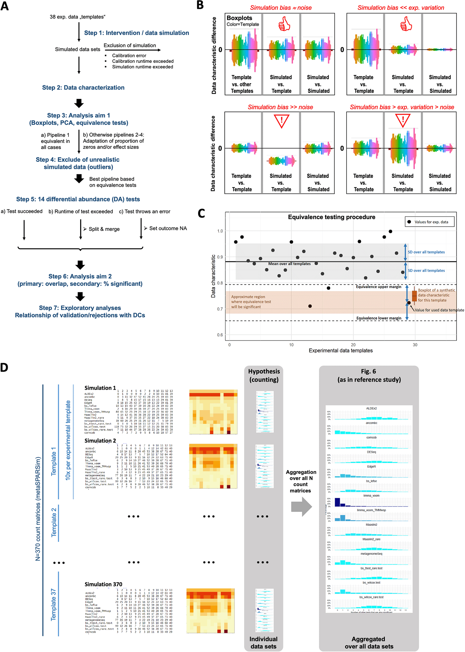
A: Overview about the analysis workflow and the exclusion/modification strategy. The depicted strategy was applied to handle runtime issues, computation errors and unrealistic simulated data. B: Illustration of the visual evaluation of the DCs. The left sections of the boxplots show the difference of a data characteristic between templates pairs, serving as a measure of the natural variability. The middle sections show for each template the difference of the DC to the 10 simulated datasets, serving as a measure of precision of data simulation. The right sections display the difference of a DC within the simulated data for one template, serving as a measure for variability due to simulation noise. C: Illustration of assessing DC similarity based on an equivalence test. The black dots indicate a data characteristic computed for experimental datasets (e.g. the proportion of zeros). Equivalence tests requires an interval that is considered as equivalent given by lower and upper margin bounds (dashed lines). We use the SD over all values from experimental templates to define these margins. The values computed from the synthetic data for a template are considered as equivalent if values below the lower margin and above the upper margin can be rejected according to the prespecified significance level. Depending on the variation of the characteristic for the synthetic data (here indicated by the boxplot), the average characteristic has to be inside a region (brown region) that is smaller than the interval between both margins. D: Illustration of the primary analyses conducted for assessing the agreement of the 13 DA tests via overlap profiles. For each count matrix, the overlap within the significant taxa is counted, shown as numbers on the left, as image in the middle and as barplot („overlap profile“) on the right. These overlap profiles can be compared and aggregated at different levels. In the reference study, they were calculated and interpreted at the aggregated level over all taxa of experimental datasets. In practice, however, the agreement obtained for a single experimental count matrix matters. We therefore evaluated how frequently different hypotheses were fulfilled at the unaggregated level.

Step 1: Intervention/Data simulation

According to standardized study design guidelines, we had to define interventions and comparator. In these terms, data generation using simulation tools is the intervention that is compared with experimental data. When defining the interventions, we had to balance the complexity and runtime of the study, with the requirements of conducting the data simulation as realistic as possible and with a sufficient sample size. Due to the complexity of our study, the huge expected computational demands, and the fact that one key aim of this study was also to introduce and emphasize the importance of formulating a study protocol specifically for computational research, we decided to restrict our study to two published simulation approaches for 16S rRNA sequencing data.

For each of the 38 experimental datasets, synthetic data was simulated using metaSPARSim³ version 1.1.2 and sparseDOSSA2⁴ version 0.99.2 as simulation tools. Simulation parameters were calibrated using the experimental data, such that the simulated data reflect the experimental data template. Both simulation approaches offer such a calibration functionality. Multiple (N = 10) data realizations were generated for each experimental data template to assess the impact of different realizations of simulation noise and to test for significant differences between interventions (in our study the simulated data) and the comparator (in our study the experimental data templates). The major calibration and simulation functions were called with the following options:

# metaSPARSim calibration:
params <- metaSPARSim::estimate_parameter_from_data(raw_data=counts, 
norm_data=norm_data, conditions=conditions, intensity_func = “mean”, keep_zeros = TRUE)

# metaSPARSim simulation:
simData <- metaSPARSim (params)
# SparseDOSSA2 calibration:
fit <- SparseDOSSA2::fit_SparseDOSSA2(data=counts, control=list (verbose = TRUE, debug_dir = “./”))
# SparseDOSSA2 simulation:
simResult <- SparseDOSSA2::SparseDOSSA2(template=fit,new_features=F, n_sample=n_sample, n_feature=n_feature)

To account for the two-group design of the data, calibration and simulation were conducted for each group independently. Specifically, the datasets were first split into two groups of samples according to the metadata. Then, calibration and simulation was performed for each group, and finally, the two simulated count matrices were merged.

Next to this default simulation pipeline three adaptions were performed to control two important data properties, namely sparsity and effect size, resulting in 4 simulation pipelines:

Pipeline 1 – Default simulation

This pipeline refers to the above described simulation procedure.

Pipeline 2 – Adaption of sparsity (proportion of zeros)

Modifying the proportion of zeros was performed by the following procedure for all synthetic datasets:

Copy and replace an appropriate number of zeros (or non-zeros) one-by-one (i.e. with the same row and column indices) from the template to the synthetic data by randomly drawing those positions.

Pipeline 3 – Adaption of effect size

Since we calibrated the simulation tools for both groups separately, all simulation parameters controlling the count distribution were different in both groups. Therefore, we anticipated that the differences between both groups might be overestimated. We therefore tried to make the simulation more realistic by modifying the effect size by the following procedure for all synthetic datasets:

isDiffAbundant = runif(n=length (pvalues)) > p.adjust(p-values, method=“BH”)

Pipeline 4 – Adaption of sparsity and effect size

Both above described modifications were applied.

Exclusion of simulation for a specific data template based on simulation performance

A simulation tool was excluded for a specific data template, if calibration of the simulation parameters was not feasible. We defined feasibility by the following criteria:

All computations in this study were performed on a Linux Debian x86_64 compute server with 64 AMD EPYC 7452 48-Core Processor CPUs. Although parts of the analyses were run in parallel mode, the specified computation times refer to runtimes on a single core.

Step 2: Data characterization

To characterize and compare datasets for aim 1, 40 DCs were calculated for each template and simulation. These characteristics were chosen such that they provide a comprehensive description of count matrices and enabling unbiased comparison between experimental and synthetic datasets. They cover for example information about the count distribution, sparsity in a dataset, mean-variance trends of features (taxa), or effect sizes between groups of samples. Tables 2 and 3 provide a detailed summary of all data characteristic and how they were calculated. To prevent overrepresentation of specific distributional aspects in assessing similarity between experimental and simulated data, we excluded redundant DCs. This was achieved by calculating rank correlations for all DC pairs across all datasets (experimental and simulated) and iteratively eliminated characteristics with a rank correlation ≥0.95.

Step 3: Assessing similarity of synthetic and experimental data – Outcome aim 1

After calculating the DCs as described in Step 2, the difference of all DCs between all synthetic datasets and the corresponding data templates were calculated as outcomes. As N = 10 simulation realizations were generated, there are 10 values for each data characteristic per experimental data template. For each characteristic that was closer to a normal distribution on the log-scale according to p-values of the Shapiro-Wilk test, we applied a log2-transformation to the respective characteristic prior to all analyses.

Principal component analysis (PCA) was then performed on the scaled DCs and a two-dimensional PCA plot was generated to summarize similarity of experimental and simulated data on the level of all computed, non-redundant DCs. An additional outcome was the Euclidean distance of a synthetic dataset to its template in the first two principal component coordinates.

Additionally, boxplots were generated, visualizing for each DC how it varied between templates, between all simulation realizations, and how templates deviate from the corresponding synthetic datasets. As illustrated in Figure 1B, these boxplots qualitatively show how well a DC was resembled by a specific simulation tool.

Equivalence tests

For assessing the similarity of the synthetic data templates, we applied equivalence tests based on two one-sided t-tests as implemented in the TOSTER R-package with a 5% significance level. The scales of different DCs are inherently incomparable; for instance, the proportion of zeros ranges between 0 and 1, while the number of features varies from 327 to 59,736. Therefore, we used the SD of the respective values from all experimental data templates as lower and upper margins. Figure 1C illustrates the equivalence testing procedure for the proportion of zeros in the whole dataset as an exemplary DC. For equivalence testing, the combined null hypothesis that the tested values are below the lower margin or above the upper margin had to be rejected to conclude equivalence. This only occurs when the average DC of synthetic data is inside both margins and not too close to those two bounds, i.e. the whole 95% CI interval of the estimated mean has to be between both margins.

Step 4: Exclusion of unrealistic simulations

For validating the prespecified hypothesis as aim 2, we excluded synthetic datasets that were not similar enough to the experimental datasets used as templates. For assessing similarity, the DCs described before and specified in detail in Table 3 were used. The goal of the following exclusion criterion was to exclude synthetic datasets that are overall dissimilar from the experimental data template, without being too stringent since the simulation tools cannot perfectly resemble all DCs and therefore a slight or medium amount of dissimilarity had to be accepted. Moreover, these slight or medium dissimilarities were exploited to study the impact of those characteristics on the validation outcomes, i.e. by investigating the association of such deviations with failures in the validation outcomes.

We expected that a few DCs are very sensitive in discriminating experimental and synthetic data, termed as highly-discriminative in the following. To prevent loss of too many datasets, such characteristics that are non-equivalent for the majority (>50%) of templates were only considered for the investigation of association between mismatch in outcome and mismatch in DCs but not for exclusion.

Using the remaining DCs, unrealistic synthetic data was excluded for the validation of prespecified hypotheses in aim 2. We defined the exclusion criteria due to dissimilarity from its template by the following criteria:

For each template the number of non-equivalent DCs across all simulation realisations were counted and the results for all templates summarized in a boxplot. Synthetic data of those templates that appeared as an outlier were removed (see Supplemental Figure 1). We used the common outlier definition from boxplots, i.e. all values with distance to the 1^st quartile (Q1) or 3^rd quartile (Q3) larger than 1.5 x the inter-quartile range Q3-Q1 were considered as outlier.

For evaluating the sensitivity with respect to exclusion, we performed an additional, secondary analysis on all synthetic datasets, regardless of similarity to the templates. As there were no changes with respect the number of validated hypotheses we did not report this further in the results section.

Step 5: Differential abundance tests and exclusion/modification of DA tests

For evaluating the hypotheses (aim 2), 14 differential abundance (DA) tests were applied to the experimental and synthetic data (ALDEx2, ANCOM-II, corncob, DESeq2, edgeR, LEfSe, limma voom (TMM), limma voom (TMMwsp), MaAsLin2, MaAsLin2 (rare), metagenomeSeq, t-test (rare), Wilcoxon test (CLR), Wilcoxon test (rare)). As outcome the number of significant features for each dataset and DA test were extracted, while significant features were identified using a 0.05 threshold for the multiple testing adjusted p-values (Benjamini-Hochberg).

These analyses were conducted for unfiltered data and for filtered data. As in,¹ filtered means that features found in fewer than 10% of samples were removed.

Inflated runtime

Datasets with a large number of features could lead to inflating runtimes for some statistical tests. If the runtime threshold for an individual test was exceeded for a specific dataset, we split the dataset, applied the test again on the subsets and afterwards merged the results. This split and merge procedure was repeated until the test runtime was below the threshold.

Here, we defined the runtime threshold to be max. 1 hour per test. Then, in a worst case scenario, for each simulation tool the 14 tests for the 10+1 datasets for each of the 38 template and taking unfiltered and filtered data into account (11,704 combinations) would need 488 days on a single core. Since we conducted the tests on up to 64 cores, such a worst case scenario would have still be manageable.

Test failure

If a DA test throwed an error we omitted the number of significant features and the overlap of significant features and reported them as NA (not available) as it would occur in practice.

Step 6: Number and overlap of significant features (aim 2)

Primary outcome (2a):

For the primary outcome (2a) the proportion of shared significant taxa between DA tools was investigated. Therefore, it was determined how many tests jointly identified features to be significant for each dataset. A barplot was generated as in Nearing et al.¹ to visually summarize how many of the 14 DA tools identified the same taxa as significantly changed. Figure 1D illustrates this visualisation. The 13 hypotheses extracted from¹ were investigated using statistical analyses at the level of individual datasets. For most cases, we counted how frequently the hypothesis holds true when counting over all simulated datasets and evaluated the lower bound of the confidence interval (CI.LB) for the estimated proportions. We used exact Clopper-Pearson intervals calculated by the DescTools R-package. The statistical procedure is summarized for each hypothesis in Supplemental Text 1.

Secondary outcome (2b):

For the secondary outcome, the number and proportion of significant taxa for each DA tool was investigated. Therefore, the number and proportion of significant features was extracted for each dataset and test individually and visualized in heatmaps. After visualization, the 14 hypotheses extracted from¹ were also investigated using the statistical analyses in Supplemental Text 2.

For the primary and the secondary analysis, CI.LB of the 95% confidence intervals for the estimated proportions of cases were used to evaluate whether the hypothesis was fulfilled. These values are easier to interpret than p-values and the significance of the p-values is strongly determined by the number of cases.

In case we found different results for the simulated data for some hypotheses, we analyzed the association of the mismatch in the outcome with the mismatch of DCs to identify DCs that could be responsible for the disagreement. To ensure independence of the scales, we performed these analyses after rank transformations. We used forward selection with a 5% cut-off criterion for p-values.

Step 7: Exploratory analysis to identify relationships of confirmation and DCs

As exploratory analysis, we identified DCs that were predictive for validating/rejecting each investigated hypothesis. First, we applied a multivariate logistic regression approach to identify the most influential DCs by step-wise forward selection algorithm. This means that starting from the null model validated ~1, the DC that improved AIC most were added, then dropping a DC and adding a further one was repeated until BIC did not improve any more. This procedure identified a minimal set of characteristics that were predictive for validating/rejecting the considered hypothesis. Then, a small decision tree was estimated based on these predictive characteristics. Recursive partitioning trees as indicated by the following pseudo-code were used.

tree_model <- rpart (confirmed ~ predictiveDC1+ predictiveDC2 + … ,
   data = df, method = “class”, control = rpart.control (maxdepth = 3))

Resulting in a hierarchy of conditions “predictiveDC > threshold” indicating the optimal rule for dividing datasets into confirmation vs. rejection.

Aim 1: Synthetic data, simulated based on an experimental template, overall reflect main data characteristics

Data simulation

For each of the 38 experimental templates, 10 synthetic datasets were generated using metaSPARSim³ or sparseDOSSA2.⁴ Following the data generating mechanism in step 1, metaSPARSim³ was able to generate synthetic data for 37 of the 38 templates, while sparseDOSSA2⁴ was able to generate data for 27 of the 38 templates. MetaSPARSim³ failed to simulate data for ArcticFreshwater because taxa variability was computed only for taxa having more than 20% of values greater than zero. This default value for filtering resulted in samples without counts > 0 leading to simulation failure. For sparseDOSSA2,⁴ we observed an inflating runtime for larger datasets. For the 11 largest datasets that have 8148 – 59736 features and 75 – 2296 samples, calibration was not feasible within the prespecified runtime limit (7 days for one data template).

Four simulation pipelines were used. In the first pipeline, data was simulated with the default configuration. In the second pipeline, the proportion of zeros was adjusted afterwards. The third pipeline involved adapting the proportion of regulated features to adjust the effect size, while in the fourth pipeline, both the proportion of zeros and the effect size were modified. Figure 2 shows how the proportion of zeros P0 as well as PERMANOVA R² as a measure for effect size changed by the adaptations in the different pipelines. Adjusting sparsity perfectly resembled the proportion of zeros (upper row) in the simulated datasets when compared with the respective templates (“sim – template”). This step also made PERMANOVA R² more realistic. Adjusting the effect size in pipeline 4 by introducing taxa without regulation between the two groups of samples, only slightly further reduced bias of PERMANOVA R-squared.

Figure 2. Impact of different simulation pipelines on precision of data characteristics.

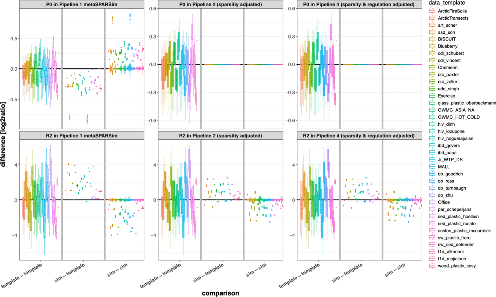
Impact of adjusting sparsity and effect size for the simulated datasets. For both simulation tools, we tried to reduce the number of non-equivalent DCs by introducing additional zeros and/or by introducing taxa without mean difference in both groups of samples. Like in Figure 1B, we show the impact of these modifications as boxplot comparing multiple experimental templates (left sections), comparing simulated with experimental data (middle sections), and comparing simulated datasets for the individual templates (right sections). Data sparsity can be adjusted to the proportion of zeros in the experimental data (upper row), but PERMANOVA effect size still deviates in simulated data compared to the experimental templates after our modifications.

Next, the set of 40 DCs was calculated for each dataset and for comparisons between datasets. The following characteristics were found as redundant (rank correlation > 0.95) and removed: q99, mean_lib_size, median_median_log2cpm, range_lib_size, mean_sample_means, SD_lib_size, mean_var_log2cpm, SD_median_log2cpm, mean_mean_log2cpm. Since the overall median was zero for all datasets and was thus also excluded, this process resulted in a final set of 30 DCs, which were used to characterize each dataset.

Individual data characteristics

Next, we visualized how well individual DCs were resembled in simulated data. Figure 3 shows boxplots of differences of DCs colored by template for metaSPARSim,³ the respective plots for sparseDOSSA2⁴ are available as Supplemental Figure 2. As illustrated in Figure 1B, the magnitude of differences between simulation and template (“simus – template”) had to be compared with variabilities between experimental templates (“templates – template”) and the variabilities of different simulation noise realizations (“simu – simu”). Overall, we did not see any DC where the differences between simulation and templates exceeded experimental variations as well as simulation noise. The DC that appeared to be the most problematic was bimodality of sample correlations (second panel in the upper row). This DC was introduced as a measure for the overall pattern caused by the two-group design. Bimodality is a DC that is sometimes difficult to estimate reliably, e.g. if two modalities (peaks) are hardly visible in the distribution. Then the estimated bimodality index could be in some cases close to zero leading to large variations if all differences are visualized as boxplot. It can be appreciated, that the mismatch of the DCs between simulated data and template was overall smaller than the span of the natural variability between experimental data.

Figure 3. Assessing the similarity of data characteristics for metaSPARSim-generated data.

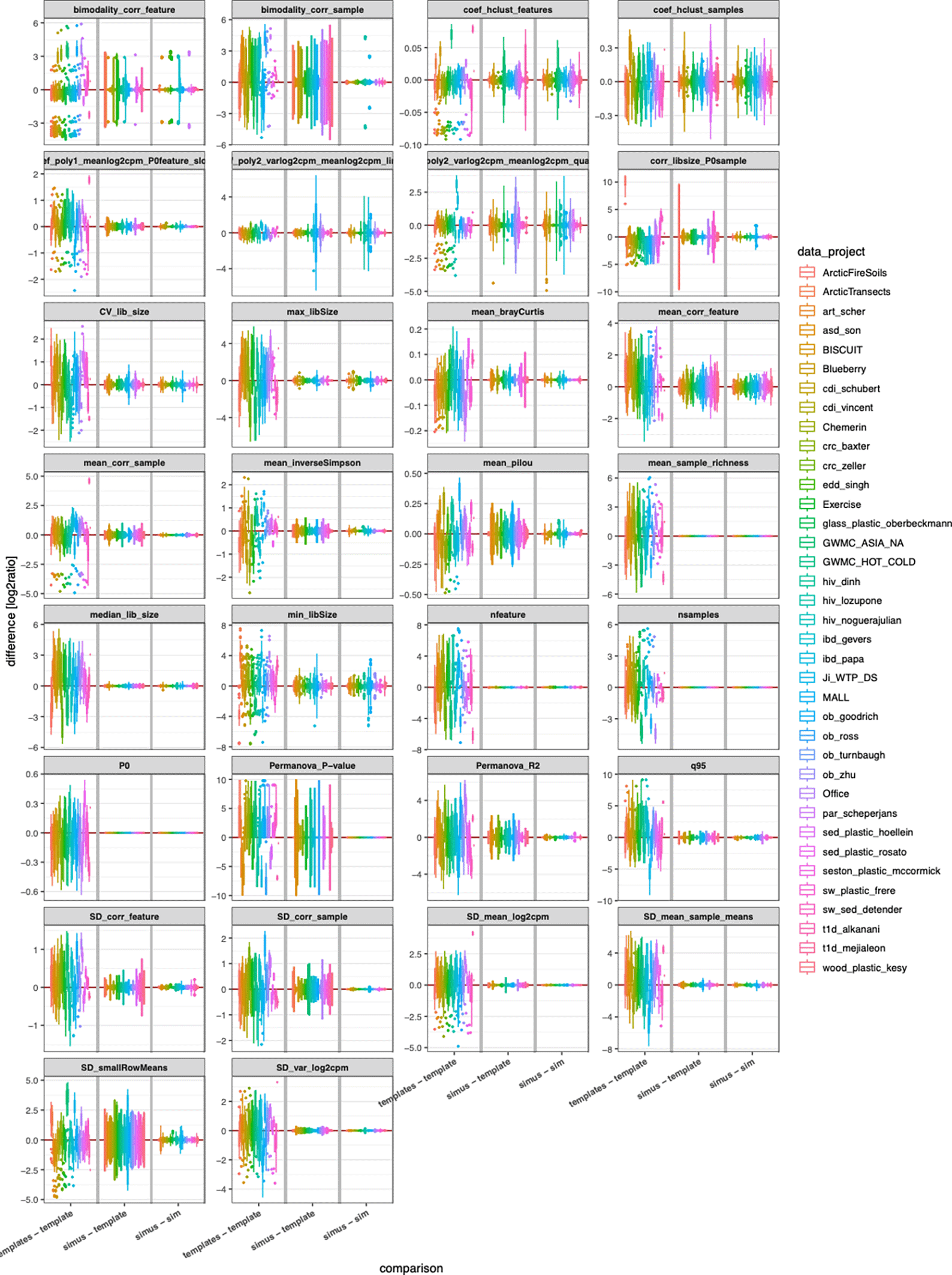
Comparison of differences of individual DCs for metaSPARSim. As in Figure 1B and Figure 2, we compared multiple experimental templates (left sections), simulated vs. experimental data (middle sections), and simulated datasets for the same template (right sections). The corresponding plots for sparseDOSSA2 are provided as Supplemental Figure 2.

Results of PCA of the data characteristics

To better assess the overall similarity of the DCs of simulated datasets with their respective templates, the 30 DCs for each dataset were analyzed and visualized by PCA. Figure 4A shows the PCA plot for metaSPARSim³ in the default pipeline 1. The simulation templates were represented as squares, with the 10 corresponding simulated datasets depicted as circles of the same color. It was evident that the synthetic datasets generated by metaSPARSim³ were typically very close to their respective templates indicating that metaSPARSim³ can reproduce DCs at this global summary level. Also, the simulation noise did not introduce significant variation, as indicated by the tight clustering of the 10 simulation realizations. The other simulation pipelines obtained similar outcomes as shown in the Supplemental Figures 3. Overall did data simulated with metaSPARSim³ closely resemble the DCs of the simulation templates.

Figure 4. PCA on scaled data characteristics assessing the similarity of real and synthetic data.

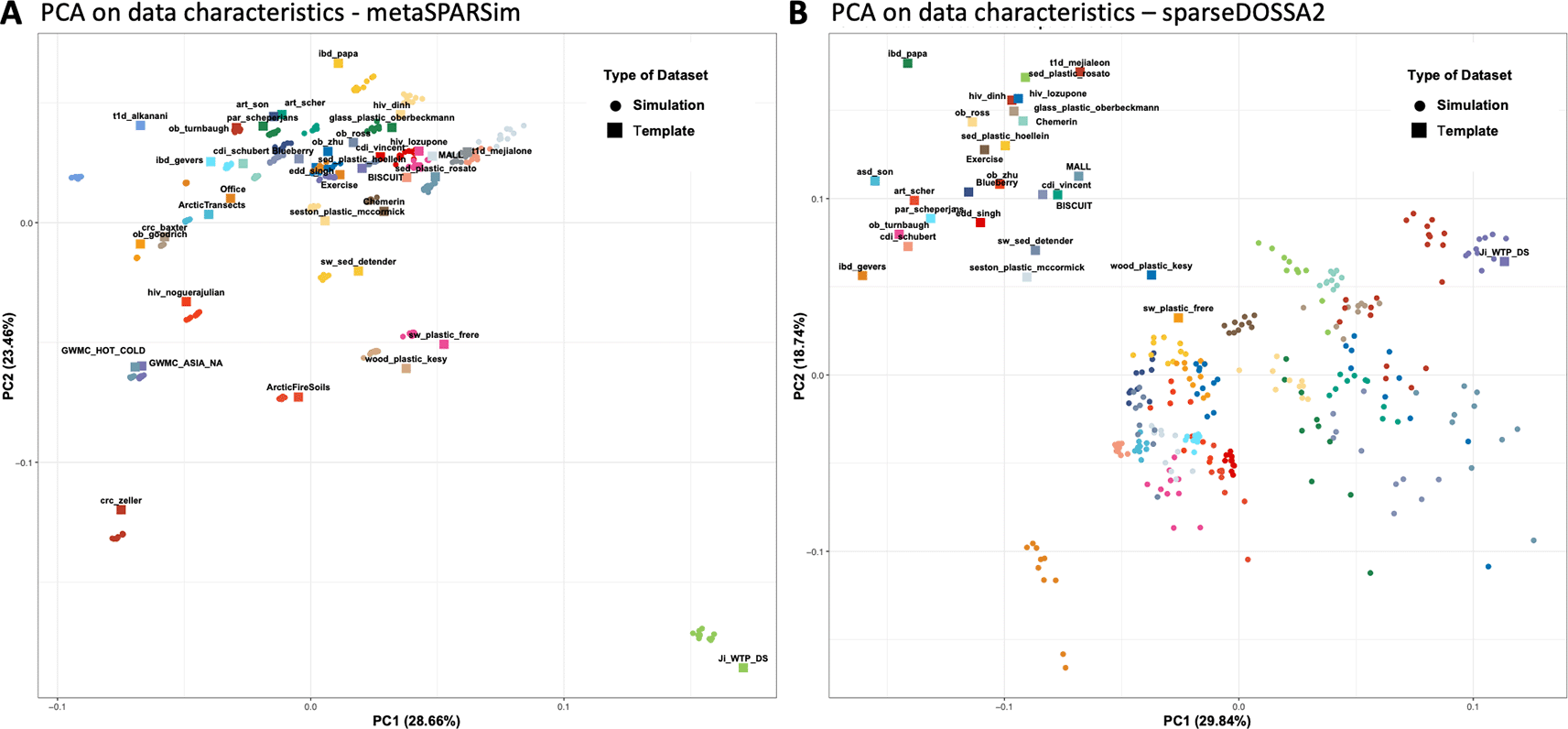
PCA on scaled data characteristics calculated for experimental and synthetic data. Experimental templates are depicted as squares, while the corresponding 10 synthetic datasets a are depicted as circles.

When using sparseDOSSA2⁴ as a simulation tool, it could be observed that the simulated data was systematically shifted towards the lower-right region of the PCA plot ( Figure 4B). Despite this, the simulation realizations for each template remained clustered together, although the clusters were less tight compared to those generated by metaSPARSim.³ This suggests that sparseDOSSA2⁴ introduces more simulation bias than metaSPARSim.³ A closer examination of the DCs responsible for the systematic shift revealed that sparseDOSSA2⁴ consistently overestimated all DCs related to library size (Supplemental Figure 2). On the other hand, sparseDOSSA2⁴ seemed to better be able to capture sparsity and effect size of a given template. Still, significance measured by PERMANOVA R-squared tended to be overestimated.

Equivalence tests

To quantitatively and more systematically assess the similarity of simulated data and their templates, equivalence tests on the DCs, testing if a given DC for a simulated dataset is within an equivalence region around the DC in the corresponding template, were performed. This resulted in one statistical test for each DC and template. The results were summarized as heatmaps ( Figure 5), displaying if the equivalence was accepted or rejected. Overall, metaSPARSim³ tended to generate data for which most characteristics were equivalent to those of the experimental templates ( Figure 5A). However, one characteristic that is often not well resolved is the sparsity of the dataset (P0). While sparsity remains equivalent to the experimental template in most cases, for 16 out of 37 templates, the sparsity did not match the value in the experimental template. These datasets typically have a low number of features (mostly below 1,000) or a moderate number (1,000-3,000), but a small number of samples (~50). As previously discussed, the bimodality of the samples was systematically overestimated in the simulated data generated by metaSPARSim.³ However, when comparing the discrepancies to the natural range in all templates, as done by the equivalence test, we noticed that only 6 templates show significant non-equivalence ( Figure 5A). This discrepancy did not seem to be linked to any obvious factors, such as sample size or the number of features. Figure 5B shows the result for the equivalence tests for metaSPARSim³ in pipeline 4, in which as well sparsity of the dataset and effect size was adjusted. It can be appreciated that this pipeline resulted in much less non-equivalent DCs and moreover resolved the issue of systematic shifts for some DCs. Figure 5C on the other hand shows the result for sparseDOSSA2⁴ in pipeline 2, in which the sparsity of the data additionally was adjusted. Confirming the results from the PCA analysis, synthetic datasets generated with sparseDOSSA2⁴ had a systematic discrepancy in DCs related to library size and distance in the PCA plot (grey bars). To identify the best data generating pipeline the number of non-equivalent DCs were counted for each pipeline ( Figure 5D). While for metaSPARSim³ pipeline 4, in which sparsity and effect size were adapted, was identified as the best choice, for sparseDOSSA2⁴ pipeline 2, in which only the sparsity was adapted, was selected.

Figure 5. Equivalence tests assessing similarity of data characteristics of real and synthetic data.

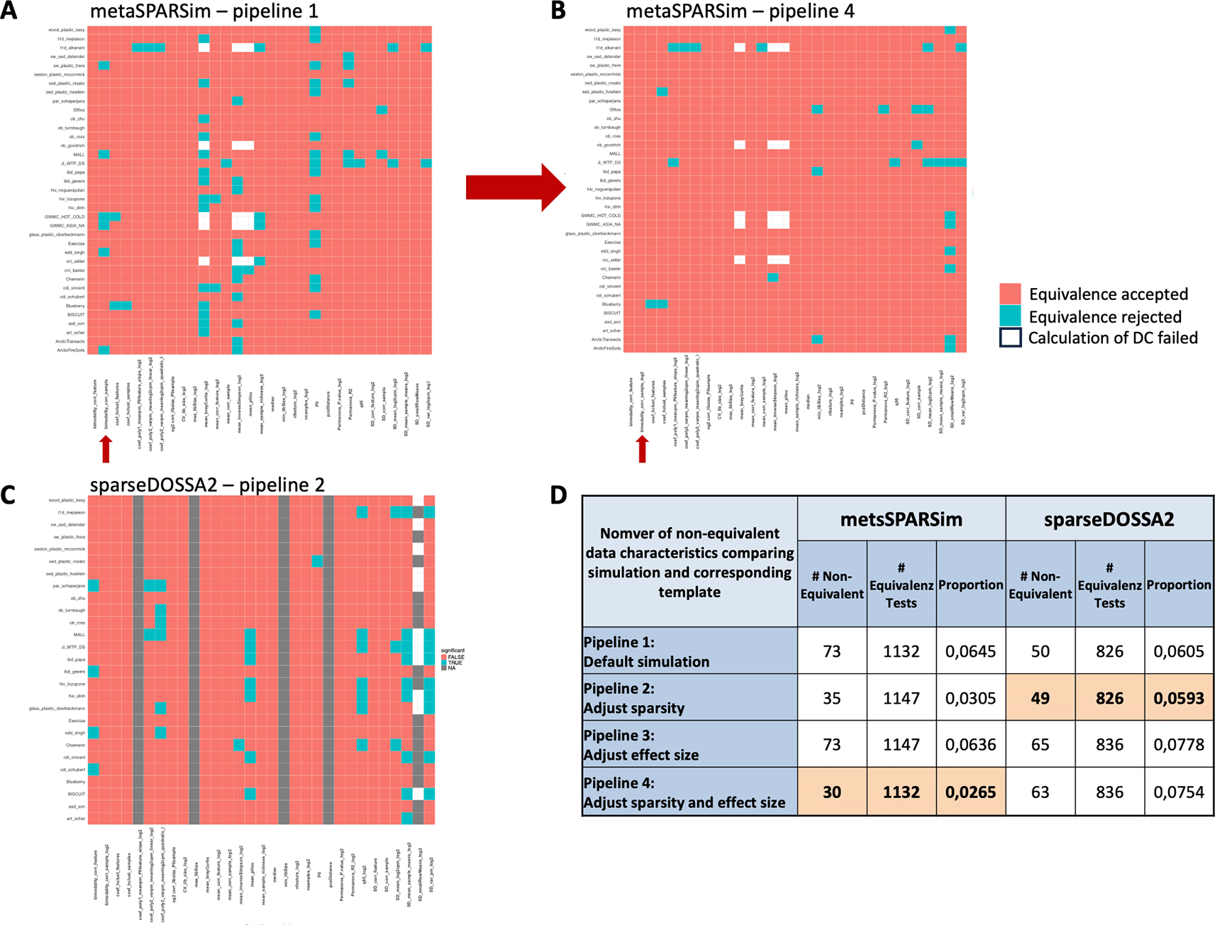
Heatmaps indicate for each data characteristic and each template if equivalence was accepted or not. A.-B. Impact on the results when sparsity and effect size in the simulation process are adapted. C. Results for the best pipeline² for sparseDOSSA2. D. Summary of the results for all simulation pipelines.

Lastly, templates with an excessively high proportion of non-equivalent DCs were removed from the selected pipelines to perform validation of our hypotheses, i.e. the conclusions in,¹ only on those simulated datasets that closely resembled the experimental templates. Supplemental Figure 1 illustrates the results for metaSPARSim³ - pipeline 4 (Supplemental Figure 1A) and sparseDOSSA2⁴ - pipeline 2 (Supplemental Figure 1B). The number of non-equivalent DCs for the simulated datasets was summarized in a boxplot. Templates identified as outliers according to the boxplot criteria were removed. For metaSPARSim,³ this led to the removal of three datasets, whereas all templates were retained for sparseDOSSA2.⁴

Aim 2: Study results from Nearing et al. can be validated using synthetic data, simulated based on corresponding experimental data

Primary outcome (2a):

The overlaps of significant features (p_FDR < 0.05) after calculating the 14 statistical tests were investigated as primary outcome. Figure 6 presents the results for both unfiltered and prevalence-filtered data. For metaSPARSim³ ( Figure 6A), the results were based on 37 datasets, while for sparseDOSSA2⁴ ( Figure 6B), they were based on 27 datasets. Consequently, a full comparison between the two pipelines was only partially feasible. Nonetheless, general trends were observed across both simulation tools that align with findings from the reference study.¹

Figure 6. Consistency profiles for differential abundance tests.

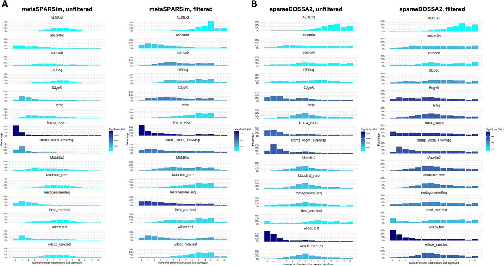
For each differential abundance test it is displayed if as significant identified taxa was also found by other tests. 0 means that no other test found this taxa while 13 means that all other test also identified this taxa to be significantly changed. The color scale shows the number of significant calls. A. Results for metaSPARSim, with results based on unfiltered data in the left panel and results for filtered data in the right panel. B. Similar visualization for sparseDOSSA2.

Overall, both simulation pipelines displayed similar trends regarding the consistency profiles of the statistical tests. Both limma-voom methods and the Wilcoxon test (CLR) identified similar sets of features that were not detected by most other tools. The consistency profiles for both Wilcoxon methods differed substantially, while those for the two MaAsLin2 approaches were very similar. Corncob, DESeq2 and metagenomeSeq exhibited intermediate profiles. ANCOM-II produced an intermediate profile for sparseDOSSA2⁴ data and a more left-shifted profile for metaSPARSim³ data, which contrasts with the reference study,¹ where ANCOM-II showed more conservative behaviour similar to ALDEx2.

For prevalence-filtered data, ALDEx2 was the most conservative tool, i.e. it had the least number of significant taxa (light color) and the most significant taxa shared with other DA methods (bars on the right), with this tendency being more pronounced for sparseDOSSA2-generated data. For filtered data, the overlap between most tests was greater compared to the unfiltered data.

As a more systematic comparison with outcomes of the reference study,¹ 13 statistical hypotheses derived from conclusions in the reference paper were tested next. Some of these hypotheses involved multiple statistical tests, which resulted in a total of 24 possible validations. The results including calculated proportions, lower bounds of the respective confidence intervals (CI.LB) were summarized in Table 4. Successful validations were colored in green, hypotheses that were true at least for the majority of simulated datasets (>50%) were colored in orange and those that were only true for the minority of cases (<50%) in red.

Validated hypotheses ( Table 4 green):

Out of the 24 hypotheses, only one could be statistically validated for both simulation tools: H1 (CI lower bound (CI.LB) metaSPARSim = 99%, CI.LB sparseDOSSA2 = 99%). This hypothesis refers to the observation that both limma-voom methods tend to identify a similar set of significant features, which differ from those identified by most other tools. Moreover, H4 could be validated for data generated with sparseDOSSA2.⁴ H4 refers to the similarity of both MaAsLin2 approaches. While this similarity was only partly evident for metaSPARSim-generated data (CI.LB metaSPARSim = 66%), it could be validated for sparseDOSSA2-generated data (CI.LB sparseDOSSA2 = 96%).

Hypotheses that were true for the majority of cases ( Table 4 orange):

For eleven validations belonging to six hypotheses we found that they were true in the majority of simulated datasets. H7 describes the intermediate consistency profile of corncob, DESeq2 and metagenomeSeq, which means that they neither tend to identify taxa that are not identified by almost no other tool and taxa that are identified by almost all other tools. For all three DA methods, we could not strictly validate this hypothesis, but we could confirm this observation for the major proportion of datasets: for Corncob we got CI.LB (metaSPARSim) = 80%, CI.LB (sparseDOSSA2) = 62%, for DESeq2 CI.LB (metaSPARSim) = 81%, CI.LB (sparseDOSSA2) = 74%, and for metageneomeSeq we have CI.LB (metaSPARSim) = 48%, CI.LB (sparseDOSSA2) = 92%.

H8 is based on the observation that in general the shape of the overlap profiles except for limma voom is quite similar for unfiltered and filtered data. Although this hypothesis could not be validated it was true for a high proportion of cases (between 72% and 83%) for all four validations.

The observation that overlap profiles of both limma voom methods shifted towards an intermediate profile for filtered data (H9), was still true for the majority of cases in our study with CI.LB between 62% and 64% of the analyzed simulated datasets.

Also H10, describing the observation that the overlap profile shifts towards a bimodal distribution in filtered data, was true in the majority of cases (CI.LB = 71% for metaSPARSim, 77% for sparseDOSSA2). The references study¹ found, that ALDEx2 and ANCOM-II in un-filtered data primarily identified taxa that were also found significant by almost all other methods (H5). For ALDEx2 this could not be strictly validated, however we found the same trend with CI.LB = 53% for metaSPARSim^3,4 and CI.LB = 60% for sparseDOSSA2. In contrast, for ANCOM-II we almost never found this behavior (CI.LB = 0% and 6%).

H3 states that the two Wilcoxon test approaches have substantially different consistency profiles. Here, we observed CI.LB = 44% for metaSPARSim³ and 72% for sparseDOSSA2.⁴ As also visible in Figure 6, this difference is more pronounced for sparseDOSSA2-generated data.

Hypotheses that are only true for the minority of cases ( Table 4 red):

Some of the hypotheses in this category are related to ANCOM-II. We observed in our data a very different behaviour of this test. Although we took the code published in the reference study,¹ this might still be related to differences in implementation, since ANCOM-II is not available as a maintained software package. In contrast to the reference study,¹ we observed that ANCOM-II shows a left-shifted to intermediate profile and not a strongly right shifted, conservative profile. Other hypotheses are related to LEfSe, which displayed a more similar consistency profile to other methods in our study compared to the reference study.¹ We also attribute this to different implementations: as for the other DA methods we used a threshold for p-values and not the score as done in the reference study.¹

We found similarity of EdgeR and LEfSe (H2) only in a minority of cases (CI.LB=15% for metaSPARSim and 21% for sparseDOSSA2). H6 and H6.1 refer to the observation that edgeR and Lefse identify a high number of unique features. In our study, we could not confirm this observations. While edgeR showed a left-shifted profile for our data, most identified features were shared with at least one other statistical test. LEfSe showed a more intermediate profile, which was even more pronounced for sparseDOSSA2-generated data.

As hypothesis 11, we intended to validate that the proportion of taxa consistently identified as significant by more than 12 tools was much higher in the filtered data than in unfiltered data. Although our overlap profiles showed this trend when all taxa are aggregated over all projects, at the level of individual datasets we only found proportions slightly above 50% (CI.LB = 52% for metaSPARSim, 55% for sparseDOSSA2).

Lastly, H12 refers to the observation that DESeq2, corncob, and metagenomeSeq exhibit intermediate profiles for unfiltered data, with a shift toward a more conservative profile for filtered data. While all three methods showed relatively intermediate consistency profiles, the impact of prevalence filtering was not as strong as in the reference study. The statistical analysis of the respective hypothesis could not confirm this at the level of individual datasets (all CI.LB of the proportions are below 3%).

Secondary outcome (2b):

For the secondary outcome the number of significant features identified by each tool was investigated. The results are displayed as heatmaps in Figure 7. We chose the same depiction as in the reference study, where colors correspond to the proportion of significant taxa per dataset, scaled over all tests (i.e. for each row) and the number of significant taxa is provided as text. Additionally, 14 hypotheses were formulated that resulted in 19 analyses, as for some hypotheses multiple DA tests had to be considered. Of these 19, we validated 10 hypotheses from the reference study, and for an additional 2 hypotheses, validation was achieved for one of the two simulation tools. For five hypotheses that concerns ANCOM-II, LEfSe, and the limma voom methods, and proportions in filtered compared to unfiltered data we found discrepancies.

Figure 7. Proportion of significant features for all tests and templates.

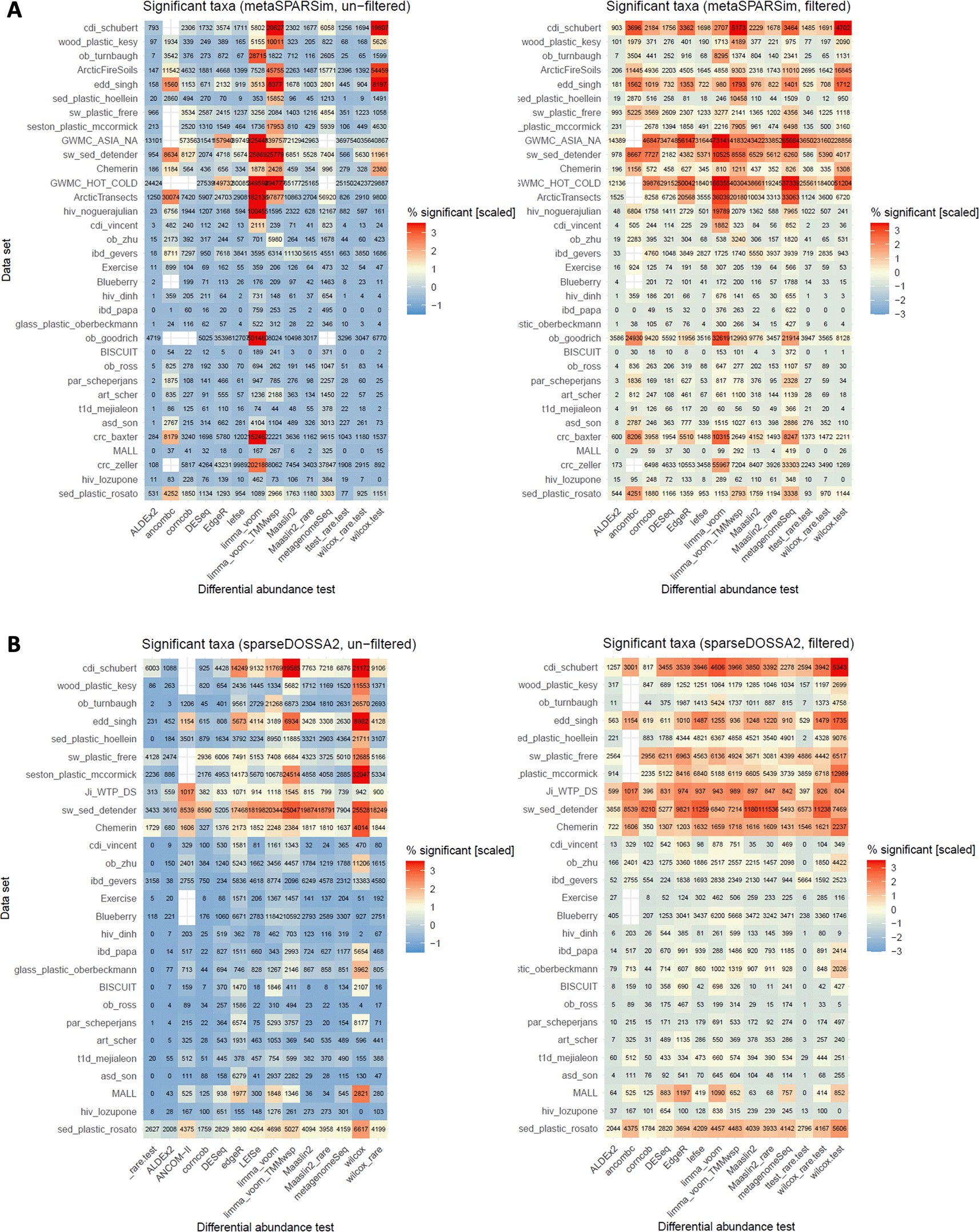
Proportion of significant features per dataset shown as a heatmap. As in the reference study, cells are colored based on the standardized (scaled and mean centered) percentage of significant taxa for each dataset. Moreover, we chose the same order of the datasets as in the reference study. The colors correspond to scaled proportions, both color scales were chosen as close as possible as in the reference study. The numbers denote the absolute number of significant features per test summed up over 10 simulated datasets. A. Result for metaSPARSim. B. Results for data generated with sparseDOSSA2.

Validated hypotheses ( Table 5 green):

Out of the 19 tests, 10 were statistically validated for both simulation frameworks. These included hypotheses H1, H2, H5, H8, and H14 with all corresponding tests. Hypothesis H1 and H2 describe the variability in DA results across the different data templates. For H1, it was confirmed that for both filtered and unfiltered data the percentage of significant features identified by each DA method varied widely across datasets. In the linear model with “test” and interaction “test:project” as predictors for the percentage of significant features, both predictors significantly contributed. This indicates that both the dataset and the DA method applied to it highly impacted the results.

Hypothesis H2 states that the percentage of significant features depends more strongly on the data template than on the method itself. Here, it was tested whether the rank of a DA method - based on the number of significant taxa - could be explained solely by the DA method, or whether significant interactions between the DA method and the data template existed. For both filtered and unfiltered data, significant interactions were observed, explaining major proportions of the total variance (p < 1e-16). Subsequent to H2, hypothesis H3 tested, whether this effect was stronger for unfiltered data. The interaction terms from H2 were compared and interestingly, this was validated for metaSPARSim³ but not for sparseDOSSA2.⁴ However, for both simulation approaches we observed that the mean squares of the interaction test:template was relatively small (MSQ_unfiltered=64 and MSQ_filtered=52 for metaSPARsim, MSQ_unfiltered=62 and MSQ_filtered=76 for sparseDOSSA2) compared to those of the main test effects (MSQ_unfiltered=3279 and MSQ_filtered=3720 for metaSPARsim, MSQ_unfiltered=2403 and MSQ_filtered=1945 for sparseDOSSA2). This resulted in slightly more test:template dependency (MSQ_unfiltered – MSQ_filtered > 0) in unfiltered data for metaSPARsim³ (in agreement with the hypothesis) but less test dependency for sparseDOSSA2⁴ (MSQ_unfiltered – MSQ_filtered < 0, i.e. discrepancy with the hypothesis). So we only found a less pronounced difference of the DA methods across projects and it was not clearly more evident in unfiltered data. This is also illustrated in the heatmaps shown in the Supplemental Figure 4.

In addition to these hypotheses, which describe a general behaviour across DA methods, four hypotheses detailing specific behaviours of DA methods were intended to be validated. Hypotheses H5 and H8 describe the observation that in unfiltered data edgeR and Wilcoxon (CLR) are tests that identify a very high or even the highest number of significant taxa for some datasets. In our simulated data, we also found such datasets. For filtered data edgeR, LEfSe, Wilcoxon (CLR) and both limma methods tended to identify the largest number of significant taxa, a trend validated in H14.

Hypotheses that were true for the majority of cases ( Table 5 orange):

For unfiltered data, the reference study¹ found, that the limma methods, Wilcoxon (CLR) or LEfSe were the DA methods that identifed the largest proportion of significant features. While this was true for the majority of our datasets, we could not strictly validate it (CI.LB = 62% and 91%).

Hypothesis H10 and H11 refer to the conservative behaviour of ALDEx2 and ANCOM-II. Specifically, they tested whether these methods do not identify significantly more features than the most conservative test in unfiltered and in filtered data. While this was true for the majority of cases in the metaSPARSim³ pipeline (CI.LB_unfiltered=79%, CI.LB_filtered=75%) and for sparseDOSSA2⁴ for unfiltered data (CI.LB_unfiltered=75%), the confidence bound was below 50% for sparseDOSSA2⁴ after prevalence-filtering (CI.LB_filtered=44%).

Hypotheses that were true for the minority of cases ( Table 5 red):

In the following, we summarize results that are only in agreement with our hypotheses for the minority of analyzed datasets and therefore do not coincide with conclusion made in the reference study.¹ Hypothesis H6 states that limma voom (TMMwsp) identifies the largest proportion of significant taxa in the Human-HIV (hiv_noguerajulian) dataset. This was never true for metaSPARSim³ generated data. However, we observed that for datasets like GWMC_Asia or GWMC_Hot_Cold limma voom (TMMwsp) consistently identified more significant taxa. These two datasets are among the largest, containing three times as many taxa than the hiv_noguerajulian dataset. For sparseDOSSA2,⁴ this hypothesis could not be validated, as calibration and therefore simulation were not feasible.

Hypothesis H7 also concerns the two limma voom methods. In the reference study,¹ these methods were reported to identify 99% of the taxa as significant for two specific datasets. In our translation of this hypothesis we generalized the behaviour, stating that for certain datasets 99% of the taxa are identified as significant. However, the datasets with observed results in the reference study,¹ were not included in our simulation pipelines due to calibration errors or unrealistic simulations. In the remaining datasets this hypothesis was not validated.

Another test that found the highest number of significant taxa for some datasets was LEfSe, which is summarized in H9. We could not validate this hypothesis. We suspect this failure is related to the different implementation and usage of LEfSe, which may have contributed to the discrepancy. In the reference study,¹ a python implementation has been used and the threshold is applied to the score to assess significance. In contrast, we used the R implementation and used p-values for calculating FDRs and assessing significance, as it is done for all other DA methods.

Another general hypothesis across most DA methods is H12. Here, we intended to validate that all tools, except for ALDEx2, identify a smaller number of significant features in filtered data compared to unfiltered data. However, for our simulated data, we had no cases where all tools (while not considering ALDEx2) indeed identified fewer significant taxa if sparsity filtering was applied. Because filtering out larger p-values would lead to smaller FDRs for small p-values, we checked whether this result is similar for unadjusted p-values. For unadjusted p-values, we found 58 out of 370 datasets where the hypothesis held true, for sparseDOSSA2 we only found 10, all of them belonging to the ob_turnbaugh template. So FDR adjustment only partly explains our surprising observation. The detailed analysis result is provided in Supplemental Table 1.

Finally, hypothesis H13, which concerns the conservative behavior of ANCOM-II in both filtered and unfiltered data, could not be validated. As discussed above, this is again attributed to discrepancies between our results and those of the reference study for ANCOM-II.

Overarching results for both, primary and secondary aims

Overall, the analyses demonstrated that synthetic data, when calibrated appropriately, can closely resemble experimental data in terms of key data characteristics (DCs). The ability of simulation tools to replicate experimental DCs was validated through principal component analysis, equivalence tests, and hypothesis-specific analyses. MetaSPARSim³ generally outperformed sparseDOSSA2⁴ in terms of replicating DCs, although both tools showed consistent trends in their ability to validate findings from the reference study.

For the primary aim (2a), which focused on validating the overlap of significant features across differential abundance (DA) tests, we confirmed few findings from the reference study. Specifically, we validated trends in the consistency profiles of limma voom, MaAsLin2, and Wilcoxon-based approaches. However, certain discrepancies were observed, particularly in the behavior of ANCOM-II and LEfSe, which deviated from expectations based on the reference study.¹ These differences may stem from variations in implementation, filtering strategies, or intrinsic differences between simulated and experimental data.

For the secondary aim (2b), which assessed the proportion of significant taxa identified by each DA method, we observed that while overall trends were mostly consistent with the reference study,¹ specific hypotheses—particularly those related to the filtering effects on DA methods—showed discrepancies. The most consistent results were found for the variation across experimental data templates, for EdgeR and Wilcoxon (CLR), while methods like ANCOM-II and LEfSe displayed notable inconsistencies.

To check, whether any conclusions concerning the investigated hypotheses depend on these two tests, we repeated the primary and secondary analyses after excluding both DA methods individually and evaluated whether the outcomes changes. For both DA methods, we found that exclusion had no impact on any validation conclusion.

We also compared the agreement of the conclusions from both simulation methods. Figure 8A shows the proportion of datasets where the hypotheses held true. It can be seen, that for both simulation tools, the results highly correlate. Moreover, we also compared these proportions for filtered and un-filtered data for hypotheses that have been claimed for both. Again, we found a strong correlation, i.e. filtering has only a minor impact on those hypotheses ( Figure 8B).

Figure 8. Association of data characteristics and validation of hypotheses.

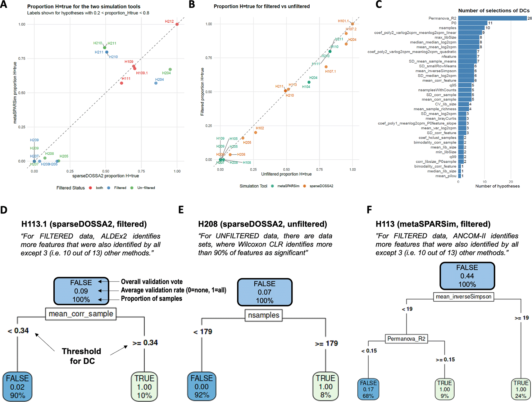
A. The proportions of datasets where the hypotheses were validated or rejected, strongly correlated for both simulation tools and (panel B) for both, filtered and un-filtered data. H1xx denote primary hypothesis xx, H2xx the secondary ones. Only hypotheses where counting over simulated datasets is applied are shown. C. Frequencies of the DCs were selected as informative for validating/rejecting hypotheses by the stepwise logistic regression approach. Effect size (PERMANOVA R-squared), the proportion of zeros (P0), and the number samples were selected most frequently. Panels D – F illustrate the decision tree analyses by three interesting examples. The percentage values indicate the proportion of all datasets and always add up to 100% on one level. The numbers indicate the average, i.e. the proportion within a branch where the corresponding hypothesis holds true.

Exploratory analysis

As an exploratory analysis, we attempted to link the outcomes of the investigated hypotheses with data characteristics. Specifically, we aimed to identify DCs that predict whether a hypothesis is validated or not across individual datasets. Identifying such relationships requires a sufficient number of cases where the hypothesis was both confirmed and not confirmed. Additionally, both outcomes should be observed across multiple templates; otherwise, any identified relationships are unlikely to generalize to unseen datasets.

Across all hypotheses and both simulation tools, PERMANOVA R-squared (26 out of 43) and the proportion of zeros (11 out of 43) were the most frequently selected predictors, followed by the number of samples in the count data (nsamples, 10 out of 43). Figure 8C illustrates the frequency with which DCs were selected. Supplemental Table 2 summarizes all predictive DCs, along with the estimated coefficients. Positive coefficients indicate that an increase in the respective DC raises the probability of a hypothesis being validated.

Next, decision trees were generated using the predictive DCs for each hypothesis. To improve interpretability, we applied a rank transformation to the DC values and scaled the ranks to the [0,1] interval to generate more intuitive meaning of the thresholds. Figure 8D presents an example for hypothesis 13.1, which holds true in only 9% of cases for all datasets (denoted as “average = 0.09” in the figure). However, for datasets with the highest 10% of the DC “mean_corr_sample” (right branch), the hypothesis is validated in all cases (“average = 1.00”). In the left branch, the hypothesis was found as false for almost all datasets (average = 0.02, 90% of datasets). A similar pattern was observed for secondary hypothesis 8, where again a decision tree with two branches was found based on nsamples as DC. After applying the denoted threshold, the hypothesis held true for all datasets in the right branch (average = 1.00 for 5% of datasets), while it was false for all datasets in the left branch (average = 0.00 for 95% of datasets).

Panel F presents a more complex decision tree where three DCs contribute. Here, two branches were identified in which hypothesis 13 was true for all datasets (average = 1.00 for 9% and 24% of datasets, respectively). However, in the third branch, the hypothesis was only valid for 17% of datasets (average = 0.17 for 68% of all datasets). Supplemental Figure 5 include decision trees for all analyzed hypotheses.

Overall, we found that certain DCs efficiently separate datasets where hypotheses hold from those where they do not. The effect size, data sparsity, and number of samples were most frequently selected as predictive factors. However, obtaining more reliable results would require a more comprehensive sampling of DCs as well as an out-of-sample validation of the derived decision rules—both would require simulated data with varying DCs which is beyond the scope of this study.