Simultaneous Numerical Determination of Two Time-dependent Coefficients in Second Order Parabolic Equation With Nonlocal Initial and Boundary Conditions

Mohammed A.J.Al-Shatrah; Mohammed Sabah Hussein

doi:10.12688/f1000research.173252.2

Home Browse Simultaneous Numerical Determination of Two Time-dependent Coefficients...

ALL Metrics

Views

Downloads

Get PDF

Get XML

Export

▬

✚

Research Article

Revised

Simultaneous Numerical Determination of Two Time-dependent Coefficients in Second Order Parabolic Equation With Nonlocal Initial and Boundary Conditions

[version 2; peer review: 3 approved, 1 approved with reservations]

Mohammed A.J.Al-Shatrah¹, Mohammed Sabah Hussein ²

PUBLISHED 03 Apr 2026

Author details Author details

¹ Ministry of Education, Directorate of Education Thi Qar, Thi Qar, 64001, Iraq
² University of Baghdad Al-Jaderyia Campus College of Science, Baghdad, Baghdad Governorate, Iraq

Mohammed A.J.Al-Shatrah
Roles: Data Curation, Formal Analysis, Investigation, Methodology, Software, Visualization, Writing – Original Draft Preparation

Mohammed Sabah Hussein
Roles: Conceptualization, Formal Analysis, Resources, Software, Supervision, Validation, Writing – Review & Editing

OPEN PEER REVIEW

REVIEWER STATUS

This article is included in the Fallujah Multidisciplinary Science and Innovation gateway.

Abstract

Background

This study establishes a mathematically consistent and computational framework for the simultaneous identification of two time-dependent coefficients in a one-dimensional second-order parabolic partial differential equation. The considered problem is governed by nonlocal initial, boundary, and integral overdetermination conditions.

Methods

The direct problem is solved using the Crank-Nicolson finite difference method (FDM), which ensures unconditional stability and second-order accuracy in both spatial and temporal discretizations. The corresponding inverse problem is reformulated as a nonlinear regularized least-squares optimization problem and efficiently solved using the MATLAB subroutine lsqnonlin from the optimization Toolbox. Due to the intrinsic ill-posedness of the inverse formulation, small input data errors lead to big output errors. Then, Tikhonov regularization is employed to enhance numerical stability and robustness.

Results

Extensive numerical experiments are carried out under exact and noisy data to evaluate the numerical accuracy and convergence behavior of the method. The results confirm that the regularization technique effectively damps numerical oscillations, minimizes reconstruction error, and ensures reliable recovery of the unknown coefficients. Sensitivity analysis further reveals the essential role of the regularization parameter in controlling the trade-off between stability and accuracy.

Conclusions

The proposed approach provides an accurate and computationally efficient tool for IP in heat transfer, diffusion processes, and related applied sciences.

Keywords

Finite difference method, Crank-Nicolson, Tikhonov regularization, Inverse problem, Coefficient problem, Ill-posed problem, Nonlocal conditions, Parabolic equation.

Corresponding author: Mohammed Sabah Hussein

Competing interests: No competing interests were disclosed.

Grant information: The author(s) declared that no grants were involved in supporting this work.

Copyright: © 2026 A.J.Al-Shatrah M and Sabah Hussein M. This is an open access article distributed under the terms of the Creative Commons Attribution License, which permits unrestricted use, distribution, and reproduction in any medium, provided the original work is properly cited.

How to cite: A.J.Al-Shatrah M and Sabah Hussein M. Simultaneous Numerical Determination of Two Time-dependent Coefficients in Second Order Parabolic Equation With Nonlocal Initial and Boundary Conditions [version 2; peer review: 3 approved, 1 approved with reservations]. F1000Research 2026, 15:228 (https://doi.org/10.12688/f1000research.173252.2) First published: 10 Feb 2026, 15:228 (https://doi.org/10.12688/f1000research.173252.1) Latest published: 03 Apr 2026, 15:228 (https://doi.org/10.12688/f1000research.173252.2)

Revised Amendments from Version 1

The revised version of the manuscript incorporates the corrections suggested by the reviewers. The introduction has been carefully revised to improve clarity and readability. Several long and complex sentences have been rewritten and simplified while preserving the scientific meaning. In discussion section, the hardware and software environment used for the computations has been added in the numerical results section. A brief discussion of the computational complexity has also been included, and it has been clarified that the reported time corresponds to a single reconstruction run. The captions of Table 1 and Table 2 have been revised to clearly indicate the unit of computational time (second). In addition, all abbreviations used in the Tables, including RMSE and objective function, have been properly defined in the revised manuscript. The wording for Example 3 has been revised to better highlight that it demonstrates both the direct problem and the corresponding inverse problem. In the new version of the article, an extensive grammar check is done, improving the clarity and coherence of the manuscript.

See the authors' detailed response to the review by Ibrahim Tekin
See the authors' detailed response to the review by Raad Awad Hameed
See the authors' detailed response to the review by Areena Hazanee
See the authors' detailed response to the review by Alla Tareq Balasim

1. Introduction

Inverse problems (IPs) arise naturally in many scientific and engineering disciplines because these systems are typically modeled by differential equations. In the context of ordinary differential equations, the direct problem refers to obtaining solutions for a given system, whereas IP focuses on reconstructing the governing system from observed characteristics. Historically, the role of IPs was recognized in celestial mechanics.¹ In practical applications, IPs are commonly encountered when one seeks to determine unknown causes from their observed outcomes, in contrast to direct problems where effects are predicted from known causes. Compared with direct problems IPs are often more difficult to solve due to their ill-posed nature. The solutions may not exist, may not be unique, or may not depend continuously on the input data.² Such problems appear in almost every scientific and technological domain, particularly in models derived from social and physical systems. Most of these models are expressed through differential and integral equations. Therefore, their analysis requires not only solving the equations but also interpreting the system behavior under different conditions, provided that sufficient information is available. IPs associated with such equations arise in a wide range of scientific and engineering applications, as well as in the modeling of social processes. Many physical phenomena are described by mathematical models in the form of initial and boundary value problems for partial differential equations (PDEs). Frequently, these models involve differential and integral equations.³ In boundary-type IPs the goal is to recover unknown boundary conditions. This often leads to classical ill-posedness because the absence of continuous dependence of the solution on the input data. Numerical solution (NS) of direct mathematical physics problems is presently a well-studied matter. In solving multi-dimensional boundary value problems, difference methods and the finite element method are widely used. PDEs from the foundation of many applied mathematical models. Their solutions are obtained by considering the govering equations together with additional relations, boundary, and initial conditions, among other elements.⁴ The following reconstruction problems serve as examples of IP applications in daily life, tomography, initial condition estimation of transient problems in conductive heat transfer, detection of non-metallic materials beneath the surface using reflected radiation methods, intensity, position estimation of illuminated radiation from a biological source using experimental radiation measures, and thermal source intensity estimation with functional dependence in space.^5–9 On the other hand, there are three different kinds of differential equations, Second-order equations are the most crucial for applications, Elliptic, Parabolic, and hyperbolic equations are examples of these equations. Yuldashev and other authors studied elliptic type integrate differential equations in^10,11 while hyperbolic and parabolic were studied in^12–14 and^15–17 respectively. The alternating direction explicit method used for reconstructing solutions is also efficient and unconditionally stable, in¹⁸ is restructured into a nonlinear regularized least-square optimization problem, and is effectively resolved using the MATLAB subroutine lsqnonlin from the optimization toolbox. The Crank-Nicolson (C-N) FDM together with the TR was used in^19–21 the effectiveness of the computational method was shown together with the proof of the solution’s existence and uniqueness. To find a stable and accurate approximate solution of finite differences. Studies in^22–26 show that IPs with a time-dependent source coefficient in heat equations acknowledge a smooth solution pair when data are available at an observation point. Moreover, providing an explicit formula for the time-dependent coefficient improves the understanding of the problem behavior. Recently, several studies have addressed inverse coefficient problems for parabolic equations with nonlocal conditions and overdetermination data. For instance, Huzyk et al. (2023)²⁷ investigated coefficient identification for strongly degenerate parabolic equations, while Azizbayov and Safarova (2025)²⁸ studied IPs for parabolic equations with nonlocal boundary conditions and two-point overdetermination. These studies further demonstrate the importance of developing stable numerical techniques for such IPs. This paper’s IP classical solution for a second order parabolic equation has been shown to be exist and unique by Elvin Azizbayov.²⁹ As a result, the main objective of the current work is a numerical realization of such a problem. This paper is organized into five sections Section 2, includes a mathematical formulation of the IP under study. Section 3, a numerical method for solving the forward problem using C-N FDM. In Section 4 the IPs mathematical solution is shown with an initial guess, while in Section 5, discuss the numerical problem and explain the obtained results.

2. Mathematical formulation

As a mathematical model, we consider $D_{T}$ be a rectangular region that is defined by $D_{T} : {(v, τ) : 0 \leq v \leq 1, 0 \leq τ \leq T}$ and $(T > 0),$ be a fixed number, the one-dimensional IP of determining of unknown functions ${w (v, τ), a (τ), b (τ)}$ for the upcoming parabolic equation,

(1)

f (v, τ) = c (τ) w_{τ} (v, τ) - w_{vv} (v, τ) - a (τ) w (v, τ) - b (τ) g (v, τ), (v, τ) \in D_{T},

with, the nonlocal initial conditions (ICs)

(2)

w (v, 0) + δw (v, T) + \int_{0}^{T} \hat{Ƥ} (τ) w (v, τ) dτ = ζ (v), v \in [0, 1],

The problem is considered with periodic boundary condition in the spatial variable v on the interval [0,1].

(3)

w (0, τ) = γw (1, τ), τ \in [0, T],

and, nonlocal integral condition

(4)

\int_{0}^{1} w (v, τ) dv = 0, τ \in [0, T],

and the overdetermination conditions

(5)

w (v_{i}, τ) = z_{i} (τ) (i = 1, 2), τ \in [0, T],

where,

γ, δ \geq 0, v_{i} \in (0, 1), (i = 1, 2); v_{1} \neq v_{2}

, are fixed numbers,

c (τ) > 0, g (v, τ), f (v, τ), \hat{Ƥ} (τ) \geq 0, ζ (v), z_{i} (τ) (i = 1, 2)

are given functions,

w (v, τ), a (τ), b (τ)

are the sought functions (

v

is space component and

τ

is time component).

2.1 Definition 1

Consider the triplet ${w (v, τ), a (τ), b (τ)}$ represents a classical solution, to the IP $(1) - (5),$ if the functions $w (v, τ), a (τ),$ and $b (τ)$ satisfies the following conditions:

1) The function $w (v, τ)$ and its derivatives $w_{τ} (v, τ), w_{v} (v, τ), w_{vv} (v, τ)$ are continuous in the domain $D_{T} .$
2) The functions $a (τ),$ and $b (τ)$ are continuous on $[0, T] .$
3) Equation (1) and conditions $(2) - (5)$ are satisfied in the classical (usual) sense.

2.2 Existence of the inverse problem classical solution

2.2.1 Theorem 1[27]: Let the assumptions $(μ 1) - (μ 4)$ and the condition

((E (T) + 2) H (T) + G (T) + Q (T)) (E (T) + 2) < 1,

where,

μ 1) ζ (v) \in C^{2} [0, 1], ζ^{(3)} (v) \in L_{2} (0, 1), ζ (0) = γζ (1), ζ^{'} (0) = ζ^{'} (1), ζ^{''} (0) = {γζ}^{''} (1);

where,

\hat{a} = \frac{1 - γ}{1 + γ}

and

\hat{b} = \frac{γ}{1 + γ}

;

γ \neq \pm 1 .

μ 2) f (v, τ) \in C_{v, τ}^{2, 0} (D_{T}), f_{vvv} (v, τ) \in L_{2} (D_{T}), f (0, τ) = γf (1, τ), f_{v} (0, τ) = f_{v} (1, τ), f_{vv} (0, τ) = γ f_{vv} (1, τ), (γ \neq \pm 1), 0 \leq τ \leq T .

μ 3) g (v, τ) \in C_{v, τ}^{2, 0} (D_{T}), g_{vvv} (v, τ) \in L_{2} (D_{T}), g (0, τ) = γg (1, τ), g_{v} (0, τ) = g_{v} (1, τ), g_{vv} (0, τ) = γ g_{vv} (1, τ), (γ \neq \pm 1), 0 \leq τ \leq T .

μ 4) δ \geq 0, c (τ) \in C [0, T], c (τ) > 0, 0 \leq \hat{Ƥ} (τ) \in C [0, T], z_{i} (τ) \in C^{1} [0, T],

z (τ) = z_{1} (τ) g (v_{2}, τ) - z_{2} (τ) g (v_{1}, τ) \neq 0, (i = 1, 2), 0 \leq τ \leq T .

where,

(6)

E_{1} (T) = 2 {(1 + δ)}^{- 1} {‖ ζ (v) ‖}_{L_{2} (0, 1)} + 2 \sqrt{T} (1 + δ {(1 + δ)}^{- 1}) {‖ \frac{1}{c (τ)} ‖}_{C [0, T]} {‖ f (v, τ) ‖}_{L_{2} (D_{T})}),

(7)

E_{2} (T) = 2 \sqrt{10} {‖ ζ^{(3)} (v) ‖}_{L_{2} (0, 1)} + 2 \sqrt{10 T} (1 + δ) {‖ \frac{1}{c (τ)} ‖}_{C [0, T]} {‖ f_{vvv} (v, τ) ‖}_{L_{2} (D_{T})},

(8)

\begin{matrix} E_{3} (T) = 4 \sqrt{3} {‖ ζ^{(3)} (v) (1 - \hat{b} - \hat{a} v) - 3 \hat{a} ζ^{(2)} (v) ‖}_{L_{2} (0, 1)} + 4 \sqrt{3 T} (1 + δ) {‖ \frac{1}{c (τ)} ‖}_{C [0, T]} \\ {‖ f_{vvv} (v, τ) (1 - \hat{b} - \hat{a} v) - 3 \hat{a} f_{vv} (v, τ) ‖}_{L_{2} (D_{T})} + 12 \sqrt{2} | \hat{a} | (1 + δ) {‖ \frac{1}{c (τ)} ‖}_{C [0, T]} {‖ ζ^{(3)} (v) ‖}_{L_{2} (0, 1)} \\ + 12 \sqrt{3} | \hat{a} | {‖ \frac{1}{c (τ)} ‖}_{C [0, T]}^{2} \sqrt{{‖ c (τ) ‖}_{C [0, T]}} T \sqrt{T} {(1 + δ)}^{2} {‖ f_{vvv} (v, τ) ‖}_{L_{2} (D_{T})}, \end{matrix}

(9)

H_{1} (T) = (1 + δ {(1 + δ)}^{- 1}) T {‖ \frac{1}{c (τ)} ‖}_{C [0, T]},

(10)

H_{2} (T) = \sqrt{6} T (1 + δ) {‖ \frac{1}{c (τ)} ‖}_{C [0, T]},

(11)

H_{3} (T) = \sqrt{6} T (1 + δ) {‖ \frac{1}{c (τ)} ‖}_{C [0, T]} + 6 \sqrt{2} | \hat{a} | {‖ \frac{1}{c (τ)} ‖}_{C [0, T]}^{2} \sqrt{{‖ c (τ) ‖}_{C [0, T]}} T^{2} {(1 + δ)}^{2},

(12)

G_{1} (T) = {(1 + δ)}^{- 1} T {‖ \hat{Ƥ} (τ) ‖}_{C [0, T]},

(13)

G_{2} (T) = \sqrt{6} T {‖ \hat{Ƥ} (τ) ‖}_{C [0, T]},

(14)

G_{3} (T) = \sqrt{3} T {‖ \hat{Ƥ} (τ) ‖}_{C [0, T]} [\sqrt{2} + 4 | \hat{a} | {‖ \frac{1}{c (τ)} ‖}_{C [0, T]} (1 + δ)],

(15)

Q_{1} (T) = (1 + δ {(1 + δ)}^{- 1}) {‖ \frac{1}{c (τ)} ‖}_{C [0, T]} \sqrt{T} {‖ b (τ) ‖}_{C [0, T]} {‖ g (v, τ) ‖}_{L_{2} (D_{T})},

(16)

Q_{2} (T) = 4 \sqrt{3 T} (1 + δ) {‖ \frac{1}{c (τ)} ‖}_{C [0, T]} {‖ g_{vvv} (v, τ) ‖}_{L_{2} (D_{T})},

(17)

\begin{matrix} Q_{3} (T) = 6 \sqrt{2 T} (1 + δ) {‖ \frac{1}{c (τ)} ‖}_{C [0, T]} ({‖ g_{vvv} (v, τ) (1 - \hat{b} - \hat{a} v) - 3 \hat{a} g_{vv} (v, τ) ‖}_{L_{2} (D_{T})} \\ + | \hat{a} | {‖ \frac{1}{c (τ)} ‖}_{C [0, T]} \sqrt{{‖ c (τ) ‖}_{C [0, T]}} T (1 + δ) {‖ g_{vvv} (v, τ) ‖}_{L_{2} (D_{T})}), \end{matrix}

where,

E_{4} (T) = E_{1} (T) + E_{2} (T) + E_{3} (T), H_{4} (T) = H_{1} (T) + H_{2} (T) + H_{3} (T),

G_{4} (T) = G_{1} (T) + G_{2} (T) + G_{3} (T), and, Q_{4} (T) = Q_{1} (T) + Q_{2} (T) + Q_{3} (T),

(18)

E_{5} (T) = {‖ {[z (τ)]}^{- 1} ‖}_{C [0, T]} {{‖ z_{1} (τ) (c (τ) {z_{2}}^{'} (τ) - f (v_{2}, τ)) - z_{2} (τ) (c (τ) {z_{1}}^{'} (τ) - f (v_{1}, τ)) ‖}_{C [0, T]} + {(\sum_{k = 1}^{\infty} {λ_{k}}^{- 2})}^{\frac{1}{2}} [2 \sqrt{2} [(1 + 4 \sqrt{3} | \hat{a} | {‖ \frac{1}{c (τ)} ‖}_{C [0, T]} (1 + δ)) {‖ ζ^{(3)} (v) ‖}_{L_{2} (0, 1)} + {‖ ζ^{(3)} (v) (1 - \hat{b} - \hat{a} v) - 3 \hat{a} ζ^{(2)} (v) ‖}_{L_{2} (0, 1)}] + 2 \sqrt{2 T} (1 + δ) {‖ \frac{1}{c (τ)} ‖}_{C [0, T]} [(1 + 6 \sqrt{2} | \hat{a} | {‖ \frac{1}{c (τ)} ‖}_{C [0, T]} \sqrt{{‖ c (τ) ‖}_{C [0, T]}} T (1 + δ)) {‖ f_{vvv} (v, τ) ‖}_{L_{2} (D_{T})}) + {‖ f_{vvv} (v, τ) (1 - \hat{b} - \hat{a} v) - 3 \hat{a} f_{vv} (v, τ) ‖}_{L_{2} (D_{T})}]] {‖ | g (v_{2}, τ) | + | g (v_{1}, τ) | ‖}_{C [0, T]} {‖ \hat{a} v + \hat{b} ‖}_{C [0, 1]}},

(19)

E_{6} (T) = {‖ {[z (τ)]}^{- 1} ‖}_{C [0, T]} {{‖ g (v_{2}, τ) (c (τ) {z_{1}}^{'} (τ) - f (v_{1}, τ)) - g (v_{1}, τ) (c (τ) {z_{2}}^{'} (τ) - f (v_{2}, τ)) ‖}_{C [0, T]} + {(\sum_{k = 1}^{\infty} {λ_{k}}^{- 2})}^{\frac{1}{2}} [2 \sqrt{2} [(1 + 4 \sqrt{3} | \hat{a} | {‖ \frac{1}{c (τ)} ‖}_{C [0, T]} (1 + δ)) {‖ ζ^{(3)} (v) ‖}_{L_{2} (0, 1)} + {‖ ζ^{(3)} (v) (1 - \hat{b} - \hat{a} v) - 3 \hat{a} ζ^{(2)} (v) ‖}_{L_{2} (0, 1)}] + 2 \sqrt{2 T} (1 + δ) {‖ \frac{1}{c (τ)} ‖}_{C [0, T]} [(1 + 6 \sqrt{2} | \hat{a} | {‖ \frac{1}{c (τ)} ‖}_{C [0, T]} \sqrt{{‖ c (τ) ‖}_{C [0, T]}} T (1 + δ)) {‖ f_{vvv} (v, τ) ‖}_{L_{2} (D_{T})}) + {‖ f_{vvv} (v, τ) (1 - \hat{b} - \hat{a} v) - 3 \hat{a} f_{vv} (v, τ) ‖}_{L_{2} (D_{T})}]] х {‖ | z_{1} (τ) | + | z_{2} (τ) | ‖}_{C [0, T]} {‖ \hat{a} v + \hat{b} ‖}_{C [0, 1]}},

(20)

H_{5} (T) = 2 T {‖ {[z (τ)]}^{- 1} ‖}_{C [0, T]} {(\sum_{k = 1}^{\infty} {λ_{k}}^{- 2})}^{\frac{1}{2}} (1 + δ) {‖ \frac{1}{c (τ)} ‖}_{C [0, T]} (1 + 3 \sqrt{2} | \hat{a} | {‖ \frac{1}{c (τ)} ‖}_{C [0, T]} \sqrt{{‖ c (τ) ‖}_{C [0, T]}} T (1 + δ)) {‖ | g (v_{2}, τ) | + | g (v_{1}, τ) | ‖}_{C [0, T]} {‖ \hat{a} v + \hat{b} ‖}_{C [0, 1]},

(21)

H_{6} (T) = 2 T {‖ {[z (τ)]}^{- 1} ‖}_{C [0, T]} {(\sum_{k = 1}^{\infty} {λ_{k}}^{- 2})}^{\frac{1}{2}} (1 + δ) {‖ \frac{1}{c (τ)} ‖}_{C [0, T]} (1 + 3 \sqrt{2} | \hat{a} | {‖ \frac{1}{c (τ)} ‖}_{C [0, T]} \sqrt{{‖ c (τ) ‖}_{C [0, T]}} T (1 + δ)) {‖ | z_{1} (τ) | + | z_{2} (τ) | ‖}_{C [0, T]} {‖ \hat{a} v + \hat{b} ‖}_{C [0, 1]},

(22)

G_{5} (T) = 2 T {‖ {[z (τ)]}^{- 1} ‖}_{C [0, T]} {(\sum_{k = 1}^{\infty} {λ_{k}}^{- 2})}^{\frac{1}{2}} {‖ \hat{Ƥ} (τ) ‖}_{C [0, T]} (1 + 2 \sqrt{3} (1 + δ) {‖ \frac{1}{c (τ)} ‖}_{C [0, T]}) {‖ | g (v_{2}, τ) | + | g (v_{1}, τ) | ‖}_{C [0, T]} {‖ \hat{a} v + \hat{b} ‖}_{C [0, 1]},

(23)

G_{6} (T) = 2 T {‖ {[z (τ)]}^{- 1} ‖}_{C [0, T]} {(\sum_{k = 1}^{\infty} {λ_{k}}^{- 2})}^{\frac{1}{2}} {‖ \hat{Ƥ} (τ) ‖}_{C [0, T]} (1 + 2 \sqrt{3} (1 + δ) {‖ \frac{1}{c (τ)} ‖}_{C [0, T]}) {‖ | z_{1} (τ) | + | z_{2} (τ) | ‖}_{C [0, T]} {‖ \hat{a} v + \hat{b} ‖}_{C [0, 1]},

(24)

Q_{5} (T) = 2 \sqrt{2 T} (1 + δ) {‖ \frac{1}{c (τ)} ‖}_{C [0, T]} {‖ {[z (τ)]}^{- 1} ‖}_{C [0, T]} {(\sum_{k = 1}^{\infty} {λ_{k}}^{- 2})}^{\frac{1}{2}} [(1 + 6 \sqrt{2} | \hat{a} | {‖ \frac{1}{c (τ)} ‖}_{C [0, T]} \sqrt{{‖ c (τ) ‖}_{C [0, T]}} T (1 + δ)) {‖ g_{vvv} (v, τ) ‖}_{L_{2} (D_{T})} + {‖ g_{vvv} (v, τ) (1 - \hat{b} - \hat{a} x) - 3 \hat{a} g_{vv} (v, τ) ‖}_{L_{2} (D_{T})} {‖ | g (v_{2}, τ) | + | g (v_{1}, τ) | ‖}_{C [0, T]} {‖ \hat{a} v + \hat{b} ‖}_{C [0, 1]},

(25)

Q_{6} (T) = 2 \sqrt{2 T} (1 + δ) {‖ \frac{1}{c (τ)} ‖}_{C [0, T]} {‖ {[z (τ)]}^{- 1} ‖}_{C [0, T]} {(\sum_{k = 1}^{\infty} {λ_{k}}^{- 2})}^{\frac{1}{2}} [(1 + 6 \sqrt{2} | \hat{a} | {‖ \frac{1}{c (τ)} ‖}_{C [0, T]} \sqrt{{‖ c (τ) ‖}_{C [0, T]}} T (1 + δ)) {‖ g_{vvv} (v, τ) ‖}_{L_{2} (D_{T})} + {‖ g_{vvv} (v, τ) (1 - \hat{b} - \hat{a} x) - 3 \hat{a} g_{vv} (v, τ) ‖}_{L_{2} (D_{T})} {‖ | z_{1} (τ) | + | z_{2} (τ) | ‖}_{C [0, T]} {‖ \hat{a} v + \hat{b} ‖}_{C [0, 1]},

where,

E (T) = E_{4} (T) + E_{5} (T) + E_{6} (T), H (T) = H_{4} (T) + H_{5} (T) + H_{6} (T), G (T) = G_{4} (T) + G_{5} (T) + G_{6} (T), and Q (T) = Q_{4} (T) + Q_{5} (T) + Q_{6} (T),

holds, then problem

(1) - (5)

, has a unique solution in the ball

K = K_{R},

of the space

{X_{k}}^{3}

, where,

λ_{k} = 2 kπ; (k = 0, 1, \dots) .

3. FDM scheme for direct (Forward) problem

The direct problem is solved in this section, where the coefficients $a (τ)$ , $c (τ)$ and $b (τ)$ are assumed to be given. To solve this problem, the Crank-Nicolson (C-N) FDM scheme is used to compute the solution of the nonlocal problem given by Equations (1)–(4) $.$ Where the domain $D_{T}$ had been divided into $M \times N$ mesh with spatial step size $∆ v = \frac{1}{M}$ and the time step size $∆ τ = \frac{T}{N}$ where $M$ and $N$ are given positive integers. The grid points have been given by

(26)

v_{i} = i ∆ v, i = \bar{0, M,}

(27)

τ_{j} = j ∆ τ, j = \bar{0, N,}

These quantities’ discretized form is given as follows,

w (v_{i}, τ_{j}) ≕ w_{i, j}, a (τ_{j}) ≕ a_{j}, b (τ_{j}) ≕ b_{j}, c (τ_{j}) ≕ c_{j}, f (v_{i}, τ_{j}) ≕ f_{i, j}, g (v_{i}, τ_{j}) ≕ g_{i, j}, and ζ (v_{i}) ≕ ζ_{i} for i = \bar{0, M,} j = \bar{0, N .}

Applying the C-N FDM, for the discretizes Equation (1) $,$ which approximated as,

(28)

\frac{w_{i, j + 1} - w_{i, j}}{∆ τ} = \frac{1}{2} ({\tilde{d}}_{j} \frac{w_{i + 1, j} - 2 w_{i, j} + w_{i - 1, j}}{{(∆ v)}^{2}} + {\tilde{a}}_{j} w_{i, j} + {\tilde{b}}_{j} g_{i, j} + {\tilde{d}}_{j} f_{i, j} + {\tilde{d}}_{j + 1} \frac{w_{i + 1, j + 1} - 2 w_{i, j + 1} + w_{i - 1, j + 1}}{{(∆ v)}^{2}} + {\tilde{a}}_{j + 1} w_{i, j + 1} + {\tilde{b}}_{j + 1} g_{i, j + 1} + {\tilde{d}}_{j + 1} f_{i, j + 1}), i = \bar{1, M,} j = \bar{0, N,}

where,

{\tilde{d}}_{j} = \frac{1}{c_{j}}

{\tilde{a}}_{j} = \frac{a_{j}}{c_{j}}

{\tilde{b}}_{j} = \frac{b_{j}}{c_{j}}

{\tilde{d}}_{j + 1} = \frac{1}{c_{j + 1}}

{\tilde{a}}_{j + 1} = \frac{a_{j + 1}}{c_{j + 1}}

, and,

{\tilde{b}}_{j + 1} = \frac{b_{j + 1}}{c_{j + 1}}

simplifying the above Equation (28), get the following difference equation,

(29)

- {\hat{A}}_{j + 1} w_{i - 1, j + 1} + (1 + {\hat{E}}_{j + 1}) w_{i, j + 1} - {\hat{A}}_{j + 1} w_{i + 1, j + 1} = {\hat{A}}_{j} w_{i - 1, j} + (1 - {\hat{E}}_{j}) w_{i, j} + {\hat{A}}_{j} w_{i + 1, j} + \frac{∆ τ}{2} \hat{H} + \frac{∆ τ}{2} \hat{D},

where,

{\hat{A}}_{j} = \frac{∆ τ {\tilde{d}}_{j}}{2 {(∆ v)}^{2}}

{\hat{A}}_{j + 1} = \frac{∆ τ {\tilde{d}}_{j + 1}}{2 {(∆ v)}^{2}}

{\hat{E}}_{j + 1} = (2 {\hat{A}}_{j + 1} - \frac{∆ τ}{2} {\tilde{a}}_{j + 1})

{\hat{E}}_{j} = (2 {\hat{A}}_{j} - \frac{∆ τ}{2} {\tilde{a}}_{j})

\hat{H} = {\tilde{b}}_{j} g_{i, j} + {\tilde{b}}_{j + 1} g_{i, j + 1}

, and,

\hat{D} = {\tilde{d}}_{j} f_{i, j} + {\tilde{d}}_{j + 1} f_{i, j + 1}

The discretization form of $(29)$ is

(30)

F (\underline{a}) = \sum_{i = 1}^{2} \sum_{j = 1}^{N} {[w (v_{i}, τ_{j}) - z_{i} (τ_{j})]}^{2} + β (\sum_{j = 1}^{N} {a_{j}}^{2} + \sum_{j = 1}^{N} {b_{j}}^{2}) .

The C-N FDM discretizes Equations (2)–(4) which approximated as,

(31)

w_{i, 0} + δ w_{i, j} + I (v_{i}) = ζ_{i}, i = \bar{1, M,}

where

I (v_{i})

is integral in Equation (2), and we have,

I (v_{i}) = \frac{∆ τ}{2} (\hat{Ƥ} (τ_{0}) w (v_{i}, τ_{0}) + \hat{Ƥ} (τ_{N}) w (v_{i}, τ_{N}) + 2 \sum_{j = 1}^{N - 1} \hat{Ƥ} (τ_{j}) w (v_{i}, τ_{j})),

Finally, the trapezoidal rule and C-N discretizes integral condition ( $4$ ) as;

(32)

w (v_{0}, τ_{j}) + w (v_{M}, τ_{j}) + 2 \sum_{i = 1}^{M - 1} w (v_{i}, τ_{j}) = 0, i = \bar{0, M}

(33)

w_{i, 0} = ζ_{i}, i = \bar{1, M,} j = 0,

(34)

w_{0, j} = γ w_{1, j}, j = \bar{0, N - 1,} i = 0,

L = {[\begin{matrix} 1 & 0 & 0 & 0 & 0 & \dots & 0 & 0 & 0 & - 2 \\ - {\hat{A}}_{j + 1} & 1 + {\hat{E}}_{j + 1} & - {\hat{A}}_{j + 1} & 0 & 0 & \dots & 0 & 0 & 0 & 0 \\ 0 & - {\hat{A}}_{j + 1} & 1 + {\hat{E}}_{j + 1} & - {\hat{A}}_{j + 1} & 0 & \dots & 0 & 0 & 0 & 0 \\ \dots & \dots & \dots & ⋱ & ⋱ & ⋱ & ⋮ & \dots & ⋮ & ⋮ \\ 0 & 0 & 0 & 0 & 0 & \dots & 0 & - {\hat{A}}_{j + 1} & 1 + {\hat{E}}_{j + 1} & - {\hat{A}}_{j + 1} \\ 1 & 2 & 2 & 2 & 2 & \dots & 2 & 2 & 2 & 1 \end{matrix}]}_{(M) х (M)},

with,

L 1 = [\begin{matrix} 0 \\ {\hat{A}}_{j} w_{1, j} + (1 - {\hat{E}}_{j}) w_{2, j} + {\hat{A}}_{j} w_{3, j} \\ {\hat{A}}_{j} w_{2, j} + (1 - {\hat{E}}_{j}) w_{3, j} + {\hat{A}}_{j} w_{4, j} \\ {\hat{A}}_{j} w_{3, j} + (1 - {\hat{E}}_{j}) w_{4, j} + {\hat{A}}_{j} w_{5, j} \\ ⋮ \\ {\hat{A}}_{j} w_{M - 2, j} + (1 - {\hat{E}}_{j}) w_{M - 1, j} + {\hat{A}}_{j} w_{M, j} \\ {\hat{A}}_{j} w_{M - 1, j} + (1 - {\hat{E}}_{j}) w_{M, j} + {\hat{A}}_{j} w_{M + 1, j} \\ 0 \end{matrix}],

and,

\hat{V} = (\hat{H} + \hat{D})

, where,

\hat{V} = [\begin{matrix} 0 \\ (b_{j} g_{2, j} + b_{j + 1} g_{2, j + 1}) + ({\tilde{d}}_{j} f_{2, j} + {\tilde{d}}_{j + 1} f_{2, j + 1}) \\ (b_{j} g_{3, j} + b_{j + 1} g_{3, j + 1}) + ({\tilde{d}}_{j} f_{3, j} + {\tilde{d}}_{j + 1} f_{3, j + 1}) \\ (b_{j} g_{4, j} + b_{j + 1} g_{4, j + 1}) + ({\tilde{d}}_{j} f_{4, j} + {\tilde{d}}_{j + 1} f_{4, j + 1}) \\ ⋮ \\ (b_{j} g_{M - 1, j} + b_{j + 1} g_{M - 1, j + 1}) + ({\tilde{d}}_{j} f_{M - 1, j} + {\tilde{d}}_{j + 1} f_{M - 1, j + 1}) \\ (b_{j} g_{M, j} + b_{j + 1} g_{M, j + 1}) + ({\tilde{d}}_{j} f_{M, j} + {\tilde{d}}_{j + 1} f_{M, j + 1}) \\ 0 \end{matrix}]

W_{j + 1} = {[w_{1, j + 1}, w_{2, j + 1}, \dots, w_{M + 1, j + 1}, w_{M, j + 1}]}^{T}, W_{j} = {[w_{1, j}, w_{2, j}, \dots, w_{M - 1, j}, w_{M, j}]}^{T}, j = \bar{0, N - 1,}

From Equation (29) $,$ with the nonlocal initial conditions $w (v, 0) = ζ (v_{i}),$ (assuming $Ƥ (τ) = δ = 0$ ), and using Equations (31)–(34), with each time step $τ_{j}$ , we can be described in matrix form as

(35)

L W_{j + 1} = L 1 W_{j} + \frac{∆ τ}{2} \hat{V}, i = \bar{1, M}, j = \bar{0, N - 1,}

the Equation (4) desired output data will be approximated using trapezoidal rule as

(36)

0 = \int_{0}^{1} H (v) w (v, τ_{j}) dv = \frac{∆ τ}{2} (w (v_{0}, τ_{j}) + w (v_{M}, τ_{j}) + 2 \sum_{k = 1}^{M - 1} w (v_{k}, τ_{j})) .

3.1 Stability and convergence analysis

The adopted C-N finite difference scheme used to solve the direct problem is unconditionally stable and second order accurate in both spatial and temporal discretization. A brief von Neumann stability analysis shows that the amplification factor satisfies $| G | = 1$ , for all mesh ratios, which guarantees the unconditional stability of the scheme. The local truncation error is of order $ϑ ({(∆ v)}^{2}, {(∆ τ)}^{2})$ confirming that the method provides second order accuracy and reliable convergence toward the analytical solution as the mesh is refined. Hence, the C-N formulation ensures both numerical stability and accuracy for the present problem.

The Crank-Nicolson finite difference scheme is well known for its unconditional stability and second-order accuracy when applied to parabolic PDEs. The stability and convergence properties of this scheme have been rigorously studied in the literature (see, for example, Samarskii and Vabishchevich⁴ and Lesnic²). Therefore the proposed numerical formulation inherits these well-established theoretical properties, ensuring reliable and stable numerical reconstruction for the present IP.

3.2 Examples for direct problem

3.2.1 Example 1: Assume an illustration for the direct problem given by $(1) - (4)$ with $D_{T} : {0 \leq v \leq 1, 0 \leq τ \leq 1},$ and the input data are,

f (v, τ) = \frac{- 1}{6} e^{τ} (1 + τ) v^{3} {(2 v - 1)}^{3} (3 v - 1) + \frac{1}{44} (133 + 1188 e^{3 τ} + 176 π^{2} (3 τ - 1) - τ (6 τ + 1)) Sin (2 πv), z (τ) = \frac{17}{256} e^{τ} (3 τ - 1), c (τ) = 1 + 9 e^{3 τ}, τ \in [0, 1], v \in [0, 1],

and, the analytical solution is,

w (v, τ) = (3 τ - 1) Sin (2 πv), g (v, τ) = e^{τ} {(2 v^{2} - v)}^{3} (3 v - 1), a (τ) = \frac{1}{44} (1 + 2 τ), with, b (τ) = \frac{1}{6} (1 + τ), (v_{1}, v_{2}) = (\frac{1}{4}, \frac{3}{4}), τ \in [0, T], (v, τ) \in D_{T}

We investigate the accuracy of the solution using diverse mesh grid size, $M = N \in {20,40,80,160}$ . In Figure 1 (a)–(d), an excellent agreement between the exact and numerical solutions can be clearly observed, indicating high accuracy. It can be noted that as the number of mesh points increases, the accuracy of the obtained solution improves, which reflects the convergence and stability of the proposed numerical scheme. Moreover, the absolute error graph at each mesh shows that the maximum magnitude of error didn’t exceed $(10^{- 5})$ , as depicted in Figure 1 (a)–(d).

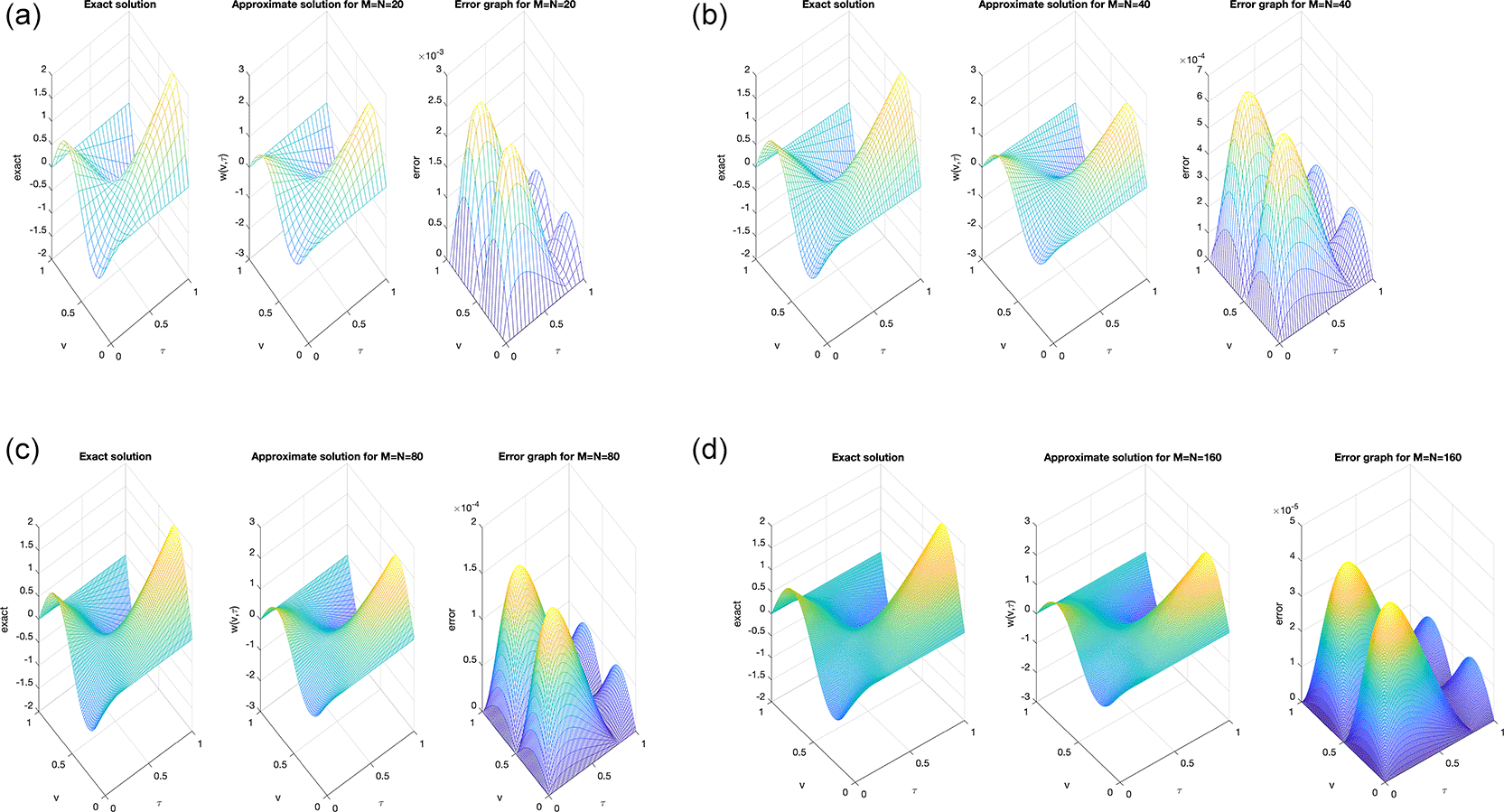
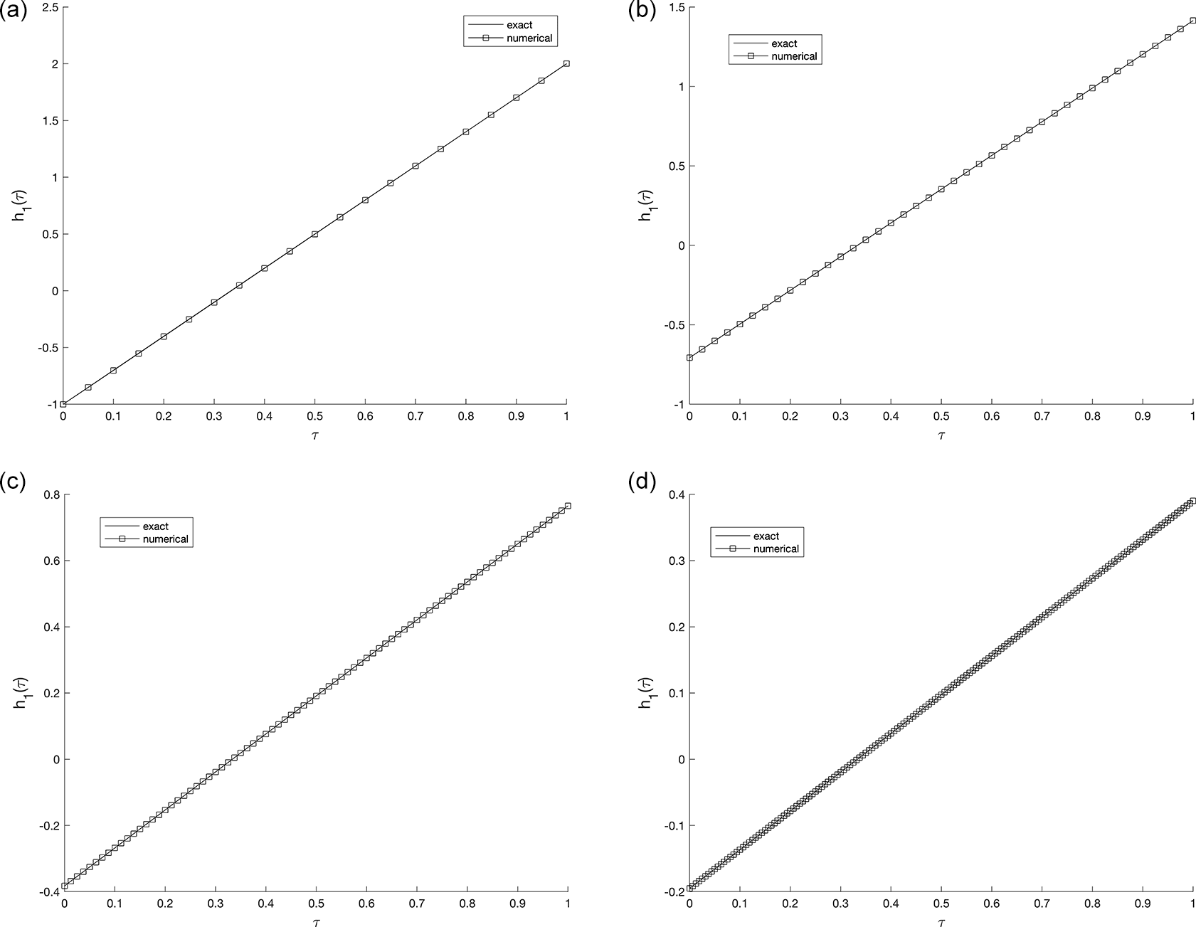
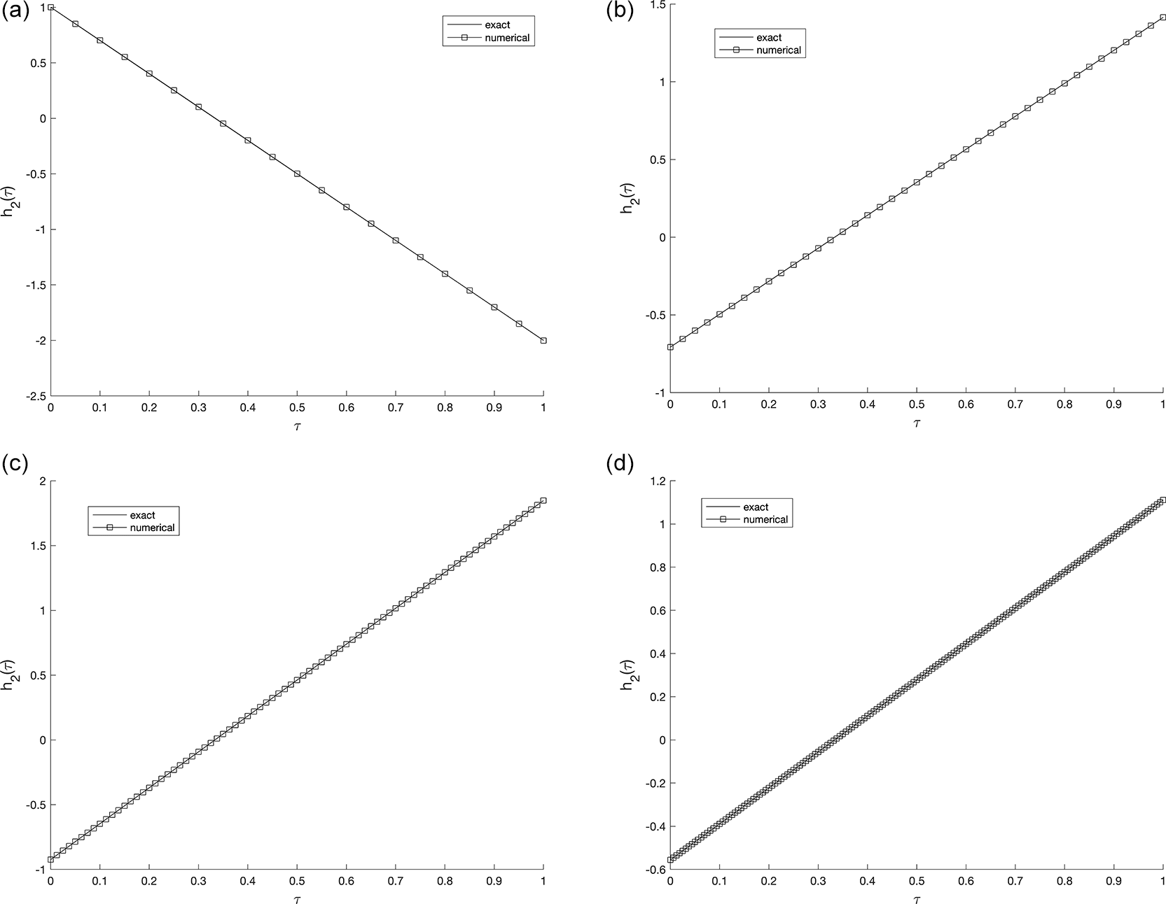
Figure 1. The graphs showing analytical and computational distribution with absolute error for the direct problem $(1) - (4)$ , for example1 $(a 1) - (d 1),$ represent the size of mesh $N = M = {20, 40, 80, 160}$ , respectively.

The obtained results clearly indicate that the mesh size has a noticeable influence on the numerical accuracy. As the spatial and temporal mesh are refined (i.e., as $M$ and $N$ increase), the numerical solution becomes smoother and shows a closer agreement with the analytical one. This behavior confirms the expected second-order convergence of the C-N finite difference scheme in both time and space. Beyond a certain refinement level (e.g., $M = N \geq 80$ ), further mesh subdivision produces only negligible changes, implying that the proposed scheme is numerically stable and nearly mesh-independent. Whilst, Figure 2 and Figure 3, show the numerical outcomes for the required information $w (v_{i}, τ), (i = 1, 2),$ evaluated at various mesh sizes such that (s.t.), observed that an excellent agreement is obtained.

Figure 2. The graphs showing the exact and numerical values for, required output $w (v_{1}, τ)$ equation $(5)$ , for example 1 $(a 2) - (d 2),$ with the size of mesh $N = M = {20, 40, 80, 160}$ , respectively.

3.2.2 Example 2: Assume an illustration for the direct problem given by $(1) - (4)$ with $D_{T} : {0 \leq v \leq 1, 0 \leq τ \leq 1},$ and the input data are,

f (v, τ) = \frac{1}{2} e^{τ} ((2 v - 1) (6 + (5 + τ) (v - 1) v) - \frac{2 Sin (πv)}{1 + τ}), z (τ) = \frac{- 3 e^{2 τ}}{32 \sqrt{2}}, c (τ) = 1,

and, the analytical solution is,

w (v, τ) = e^{τ} (1 - v) (v - \frac{1}{2}) v, g (v, τ) = e^{τ} Sin (πv), a (τ) = 6 + τ, with, b (τ) = \frac{1}{(1 + τ)}, (v_{1}, v_{2}) = (\frac{1}{4}, \frac{3}{4}), τ \in [0, T], (v, τ) \in D_{T}

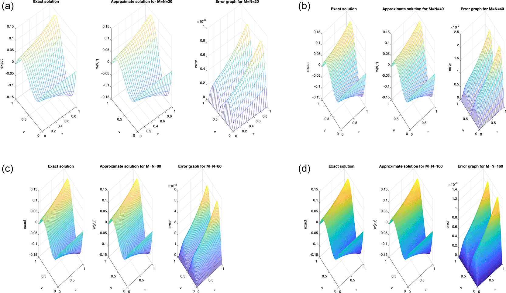
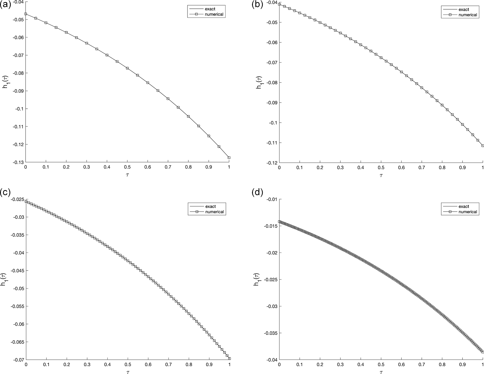
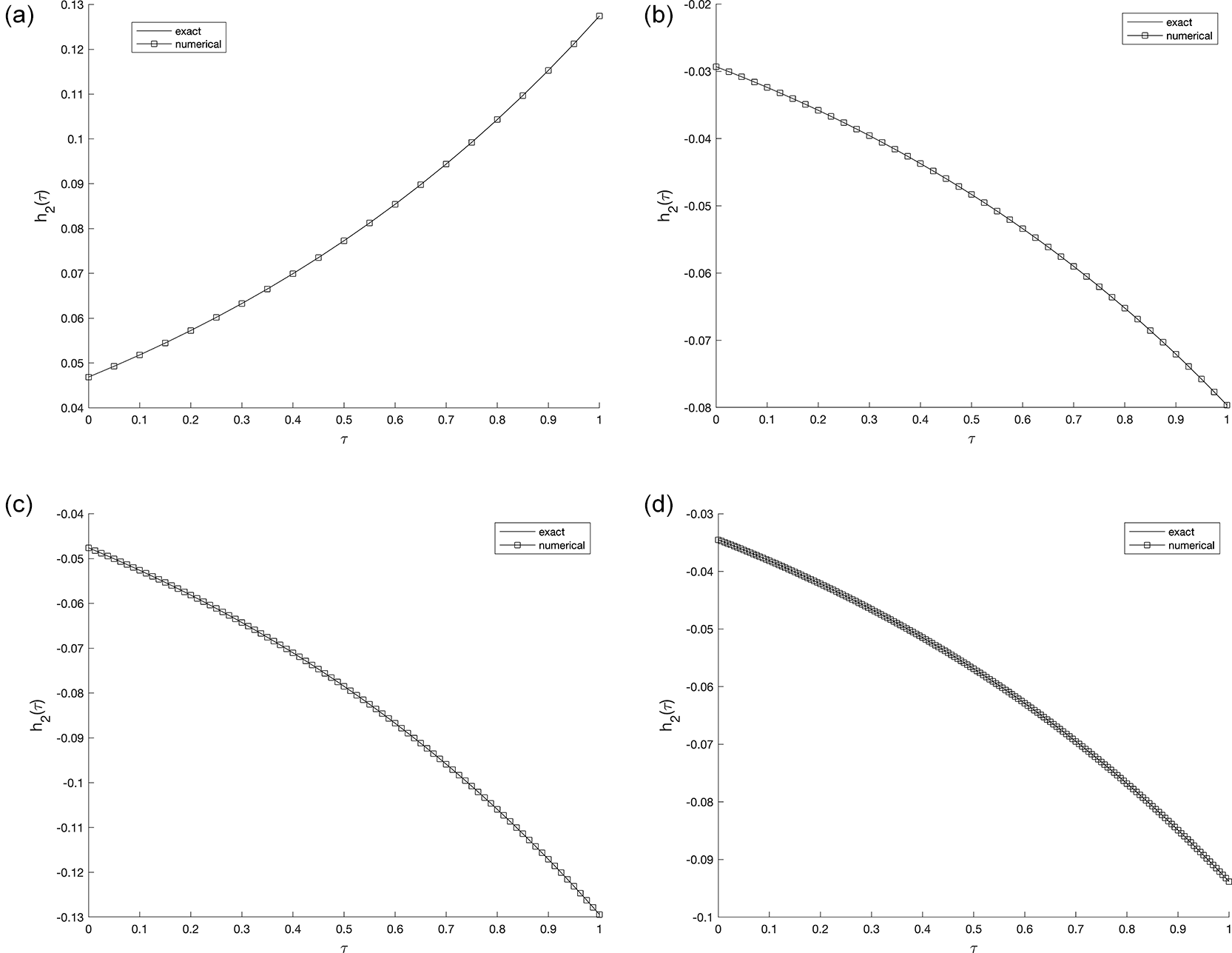
The accuracy of the numerical solution is examined using several mesh grid size, $M = N \in {20,40,80,160}$ . Figure 4 (a)–(d), clearly demonstrates an excellent agreement between the analytical and numerical solutions, confirming the reliability of the proposed approach. It can be noted that as the number mesh becomes finer, the numerical accuracy improves, indicating the expected convergence and stability of the C-N finite difference scheme. Furthermore, the absolute error plots at different mesh sizes reveal that the maximum error magnitude remains below $(10^{- 8})$ , as illustrated in Figure 4 (a)–(d).

Similarly, in Example 2, the refinement of the spatial and temporal mesh has a direct impact on the numerical accuracy. As the grid is successively refined, the computed solution aligns more closely with the analytical one, and the absolute error distribution becomes smoother across the domain. This confirms that the proposed C-N finite difference formulation maintains its second-order convergence and numerical stability. It can therefore be concluded that the results are consistent and nearly insensitive to further mesh refinement beyond the tested resolutions, indicating satisfactory mesh-independence of the method. Whilst, Figure 5 and Figure 6, show the numerical outcomes for the required information $w (v_{i}, τ), (i = 1, 2),$ evaluated at various mesh sizes s.t. observed that an excellent agreement is obtained.

Figure 3. The graphs showing the exact and numerical values for, required output $w (v_{2}, τ)$ equation $(5)$ , for example 1 $(a 3) - (d 3),$ with the size of mesh $N = M = {20, 40, 80, 160}$ , respectively.

Figure 4. The graphs showing analytical and computational distribution with absolute error for the direct problem $(1) - (4)$ , for example2 $(a 4) - (d 4),$ represent the size of mesh $N = M = {20, 40, 80, 160}$ , respectively.

Figure 5. The graphs showing the exact and numerical values for, required output $w (v_{1}, τ)$ equation $(5)$ , for example 2 $(a 5) - (d 5),$ with the size of mesh $N = M = {20, 40, 80, 160}$ , respectively.

Figure 6. The graphs showing the exact and numerical values for, required output $w (v_{2}, τ)$ equation $(5)$ , for example 2 $(a 6) - (d 6),$ with the size of mesh $N = M = {20, 40, 80, 160}$ , respectively.

4. Inverse problem solution for Equations (1)–(5)

For the nonlinear IP $(1) - (5),$ we seek precise and stable identification of $w (v, τ), a (τ)$ and $b (τ)$ , that mean potential term $a (τ)$ , and $b (τ)$ is unknown. The one-dimensional second-order parabolic equation together with $w (v, τ)$ satisfies the problem given by Equation (1)–(5), the problem is reformulated as a nonlinear least-squares minimization task. The resulting minimization problem is solved numerically using the lsqnonlin routine available in MATLAB’s optimization Toolbox, which implements a trust-region reflective algorithm suitable for nonlinear least squares problems with bound constraints. Due to the ill-posedness of such problems, especially in the presence of noise data, Tikhonov Regularization (TR) is employed to stabilize the solution. The regularization parameter $β \geq 0$ , is selected carefully to balance the trade-off between measured and the numerically computed solution. For this purpose, MATLAB routine lsqnonlin is employed, to minimize the Tikhonov Regularized objective functional, the procedure begins with a suitably selected initial guess. The TR functional is derived based on condition $(5)$ , and the functional error is incorporated as follows:

(37)

F (a) = \sum_{i = 1}^{2} {‖ w (v_{i}, τ) - z_{i} (τ) ‖}^{2}_{L^{2} [0, τ]} + β ({‖ a (τ) ‖}^{2}_{L^{2} [0, τ]} + {‖ b (τ) ‖}^{2}_{L^{2} [0, τ]}),

where $β > 0,$ is a regularization parameter.

The unregularized case, i.e., $β = 0,$ produces the regular a nonlinear least-squares functional, which is inherently unstable when dealing with noisy data. The MATLAB routine lsqnonlins is used to minimize $F$ under some physical constraint. The following parameters had been used for the subroutine:

• (Maxlter) maximum number of iterations $= 10^{6} х (N)$ .
• Solution and Objective function tolerance $= 10^{- 10}$
• The lower and upper bounds on the component of the vector $\underline{a}$ are $- 10^{- 2}$ and $10^{2}$ , respectively.

The IP $(1) - (5)$ are resolved via both precise and noisy measurement $(5)$ . By including a random error, the noisy data is numerically simulated:

(38)

z^{ε} (τ_{j}) = z (τ_{j}) + ε_{j} j = \bar{0, N .}

where

ε

, is random Gaussian normal distribution vectors with mean zero and standard deviations

σ

, given by

(39)

σ = ρ х {max}_{τϵ [0, T]} | z (τ) |

where,

ρ

is the percentage of noise. We use the MATLAB function “normrnd”, as:

(40)

\underline{ε} = normrnd (0, σ, N),

to generate the random variables

\underline{ε} = (ε_{j})

and,

j = \bar{0, N .}

5. Results and discussion

To evaluate the precision and stability of the numerical methods, a set of numerical experiments is conducted. These experiments are designed to evaluate the accuracy of the computed results by simulating realistic measurement conditions, where noise is introduced into the input data. To quantitatively evaluate the discrepancy between the exact and the numerically computed solutions, the root mean squares errors (RMSE) are utilized by the following expression

(41)

RMSE (a) = \sqrt{\frac{1}{N} \sum_{i = 1}^{N} {(a_{i}^{exact} - a_{i}^{numerical})}^{2}},

we take,

T = 1

for simplicity.

5.1 Example 3: Illustrates the solution of the IP together with the corresponding direct problem in order to demonstrate the effectiveness of the proposed regularization approach

Consider the IP $(1) - (5)$ with the following input data,

f (v, τ) = (- 2 + 4 π^{2} (3 + τ) - τ (7 + 2 τ)) Sin (2 πv) - τ^{2} (7 + 2 τ) Sin (4 πv), τ \in [0, T],

z (τ) = \frac{- 1}{4} \sqrt{15 + \sqrt{5 (33 - 8 \sqrt{2})}} (3 + τ) (7 + 2 τ), c (τ) = 1, τ \in [0, T],

where

γ = 2

, and, the analytical solution for this IP is provided as follows,

w (v, τ) = (3 + τ) Sin (2 πv), g (v, τ) = (7 + 2 τ) Sin (4 πv), a (τ) = 2 τ + 1, with, b (τ) = τ^{2}, (v_{1}, v_{2}) = (\frac{1}{8}, \frac{2}{5}), τ \in [0, T], (v, τ) \in D_{T}

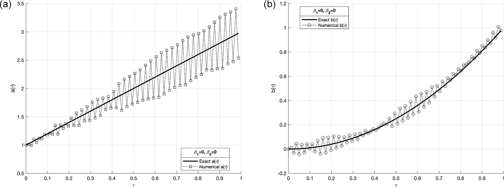
The time-dependent coefficient $a (τ)$ , and $b (τ)$ , are then reconstructed (in case, $M = N = 80$ , is taken), and consider the case of noise-free in the measurements, see Table 1, this mean $p = 0,$ in $(37)$ and, no regularization applied, Figure 7 shows the objective function $(37)$ without regularization i.e. $β = 0,$ while, in Figure 9, noise without regularization.

Table 1. Numerical reconstruction results for the IP showing the mesh size (M=N), root mean square error (RMSE) of the reconstructed coefficients and information for no regularization $β = 0$ and noise $p = 0$ .

$M = N$	80
RMSE a( $τ$ )	0.0241
RMSE b( $τ$ )	2.1592 $\times 10^{- 4}$
Computational time (second)	3594 Sec
Number of Iterations	16
Objective Function value	1.2221× $10^{- 10}$

Figure 7. The graph showing the objective function for the IP $(1) - (5)$ , in example 3 when the size of mesh $N = M = 80$ .

Figure 8. The graphs $(a 8)$ and $(b 8)$ showing the reconstructed coefficient $a (τ)$ and $b (τ)$ in comparison with exact value for the IP $(1) - (5)$ , in example 3 when the size of mesh $N = M = 80$ .

Figure 9. The graph showing the objective function when $p = 0.01 %,$ no regularization for the IP $(1) - (5)$ , in example 3, when the size of mesh $N = M = 80$ .

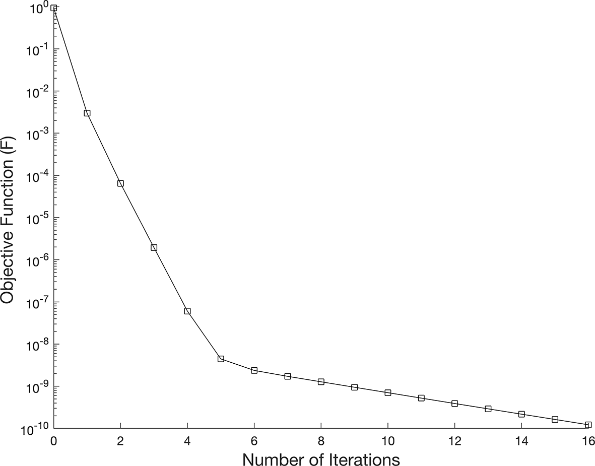
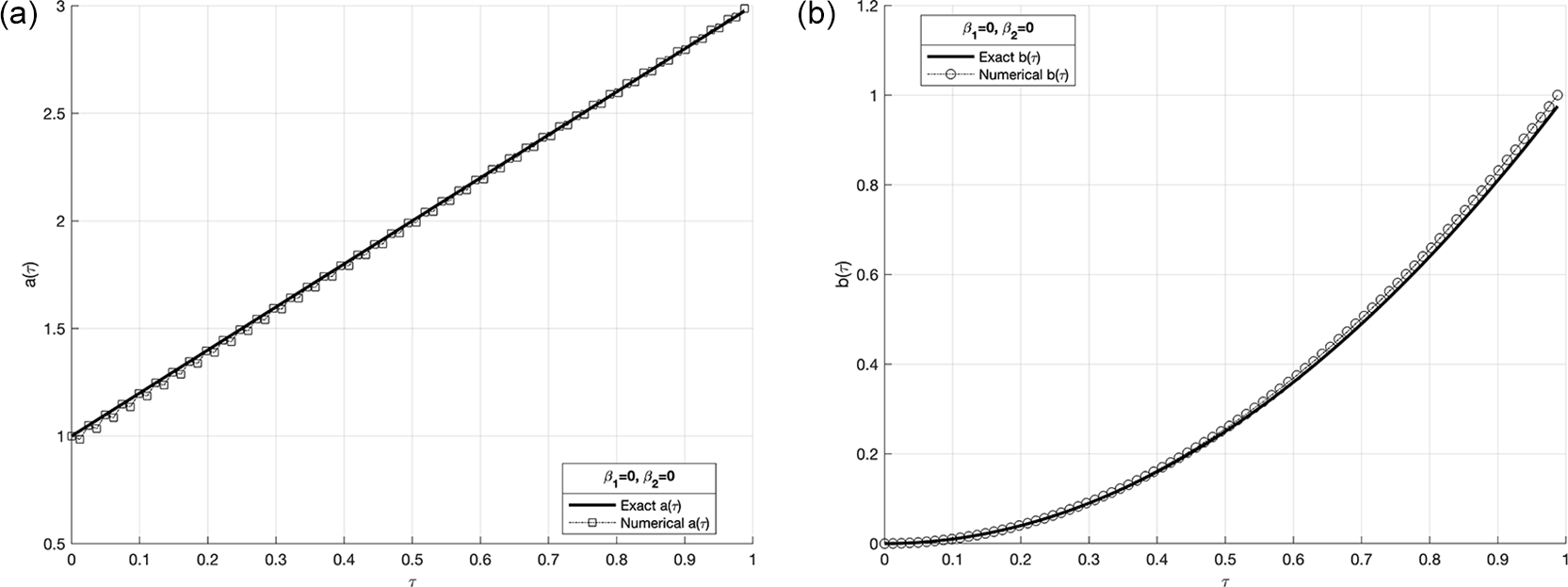
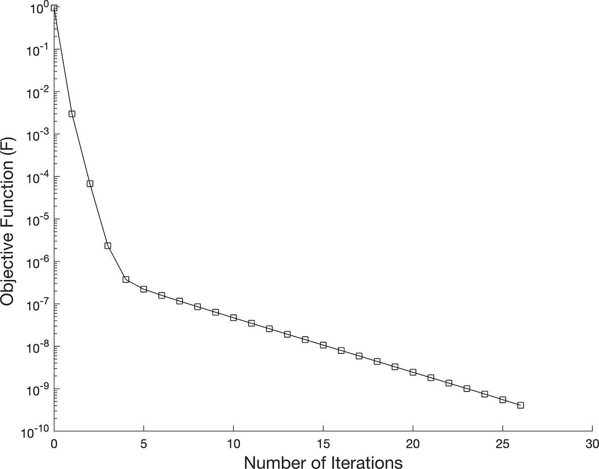
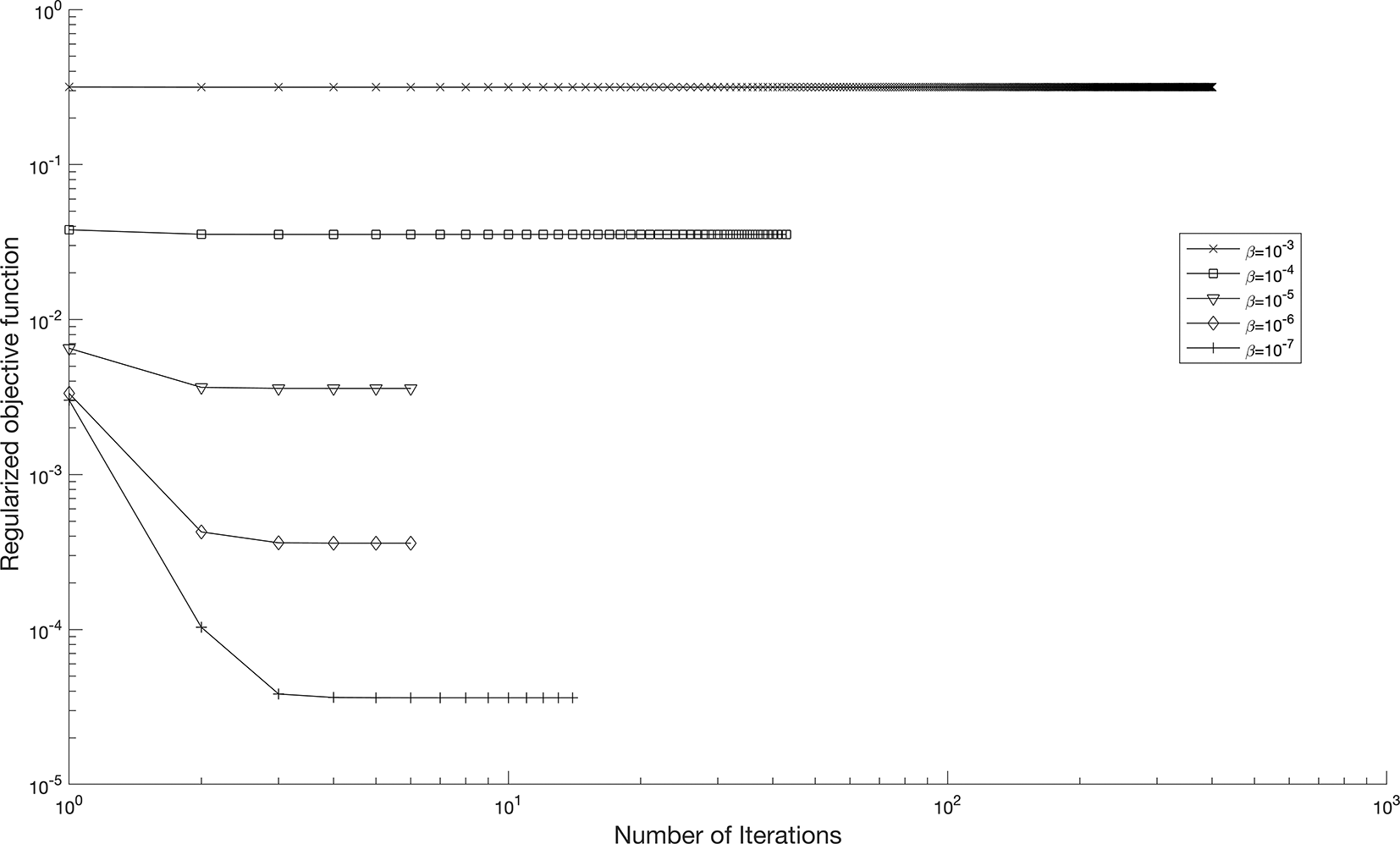
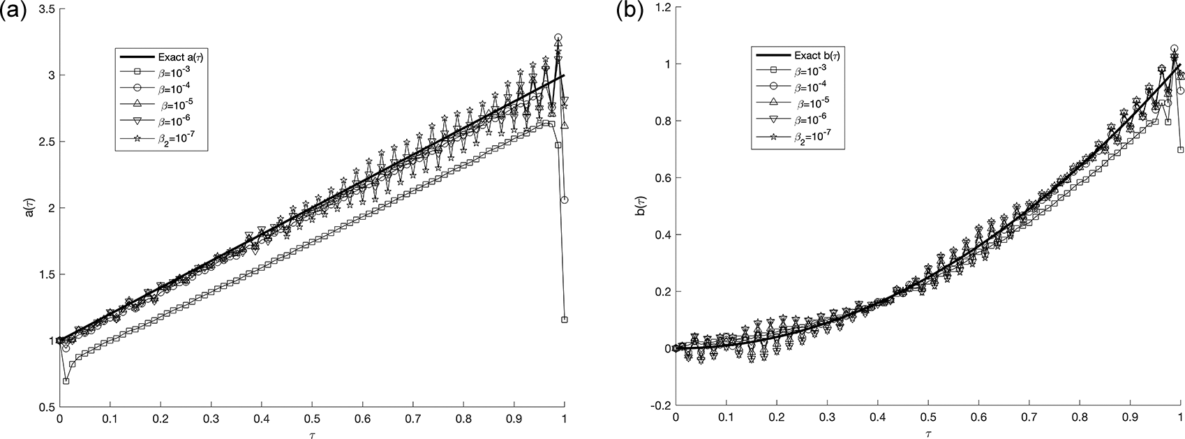
We investigate the time-dependent coefficient $a (τ)$ and $b (τ)$ under both exact and perturbed measurements, as demonstrated in Figures 7 $-$ 12. The associated results are unstable, as illustrated in Figure 9- Figure 10. This reveals that the problem is not properly posed, a noticeable instability appears in the results, which is anticipated due to the ill-posed nature of the investigated IP. The unregularized solutions exhibit noticeable instability even in the noise-free case, demonstrating the sensitivity of the problem to small perturbations in the input data. The TR approach is used by incorporating the penalty term $β ({‖ a (τ) ‖}^{2}_{L^{2} [0, τ]} + {‖ b (τ) ‖}^{2}_{L^{2} [0, τ]})$ into the classical least-squares formulation, as presented in Equation (37). In Figure 11, $p = 0.01 %$ noise strategy is employed to enhance the solution’s robustness with regularization parameters, $β \in {10^{- 3}, \dots, 10^{- 10}}$ , yielding numerically stable regularized reconstructions of $a (τ)$ and $b (τ)$ , as shown in Table 2, where the results for the case with noise level p=0% are provided in Table 1. In the following figure, Figure 12 illustrates the influence of different values of the regularization parameter β on the reconstructed coefficients a(τ) and b(τ) in the presence of noisy data. The results show that the regularization method stabilizes the solution, with smaller values of $β$ proving effective when the data is not contaminated.

Figure 10. The graphs $(a 10)$ and $(b 10)$ showing the exact and (unstable) numerical solution for $a (τ)$ and $b (τ)$ when $p = 0.01 %,$ no regularization for the IP $(1) - (5)$ , in example 3, when the size of mesh $N = M = 80$ .

Figure 11. The graph showing the objective function when $p = 0.01 %$ noise with regularization, $β \in {10^{- 3}, \dots, 10^{- 7}}$ , for the IP $(1) - (5)$ , in example 3, when the size of mesh $N = M = 80$ .

Figure 12. The graphs $(a 12)$ and $(b 12)$ showing the exact solution and regularized numerical reconstructions of $a (τ)$ and $b (τ)$ when $p = 0.01 %,$ and several curves corresponding to different values of the regularization parameter $β \in {10^{- 3}, \dots, 10^{- 7}}$ are presented to illustrate the influence of the regularization parameter on the stability of the reconstructed solution, for the IP $(1) - (5)$ , in example 3, when the size of mesh $N = M = 80$ .

All numerical computations were performed using MATLAB R2022a on a personal computer equipped with Intel Xeon E-2186M processor and 32 GB RAM, running windows 11 Pro for Workstations (64-bit). The computational complexity of the proposed algorithm mainly arises from solving the discretized parabolic equation at each iteration together with the nonlinear least-squares optimization procedure. The reported computational time corresponds to a single reconstruction run.

Table 2. Numerical results for different values of the regularization parameters with noise $p = 0.01 %, (N = 80$ ) and grid size.

$β$	$10^{- 3}$	$10^{- 4}$	$10^{- 5}$	$10^{- 6}$	$10^{- 7}$	$10^{- 8}$	$10^{- 9}$	$10^{- 10}$
RMSE a( $τ$ )	0.3302	0.1220	0.0714	0.0617	0.1189	0.2408	0.2835	0.2865
RMSE b( $τ$ )	0.0552	0.0225	0.0259	0.0344	0.0365	0.0373	0.0377	0.0377
Computational time (second)	84320 Sec	9211 Sec	1453 Sec	1451 Sec	3139 Sec	6277 Sec	5814 Sec	5506 Sec
Number of Iterations	401	43	6	6	14	22	22	22

Next, we will study the proportion of noise contamination with a ratio of $p = 0.01 %$ noise, in $(38)$ via $(39)$ , the associated results are unstable, as illustrated. This reveals that the problem is not properly, posed and small error in the data input cause large errors in the output solution, thus, the problem needs to be regularized. As a consequence, for the situation of $p = 0.01 %$ noise, the best selection for the regularization parameters is $10^{- 6}$ for $a (τ)$ and $10^{- 4}$ for $b (τ)$ as in Table 2, which results in the lowest RMSE values.

6. Conclusions

In this study, the identification of the unknown time-dependent coefficient $a (τ)$ and $b (τ)$ in a one-dimensional parabolic PDE are investigated. The problem is formulated from a numerically evaluated nonlocal integral subjected to initial and boundary conditions. The direct problem is solved using the Crank-Nicolson (C-N) scheme, while the IP is transformed into a nonlinear least squares optimization problem using the lsqnonlin routine in MATLAB. An example test cases are employed in numerical experiments to evaluate the accuracy and stability of the proposed method. According to the results, using TR significantly enhances the solution’s stability. When the root-mean square error (RMSE) numbers are their lowest, the most effective approach is identified. Furthermore, numerical results have been provided to illustrate the accuracy and stability of the numerical method. It found that applying TR method stabilizes the solution. Cases of numerical results exist with noise (with and without) regularization. In the first case, consider when $p = 0.01 %$ noise and without regularization as in Figure 9- Figure 10 in example 3, the results are unstable and highly oscillated, on the contrary. Other case, when $p = 0.01 %$ noise introduced with $β \in {10^{- 3}, \dots, 10^{- 10}},$ regularization, obtain are stable and accurate results for the reconstructed coefficient $a (τ)$ and $b (τ)$ , which are (stable) numerical solutions. As for the remaining cases, we observe that the results are stable and steady when regularization values are $10^{- 6}$ for $a (τ)$ and, $10^{- 4}$ for $b (τ)$ in example 3, as shown in Table 2.

Data availability

Data sharing not applicable to this article as no datasets were generated or analyzed during the current study.

References

1. Llibre J, Ramirez R: Inverse Problems in Ordinary Differential Equations and Applications. Progress in Mathematics. 2016; 313. 978-3-319-26337-3, 978-3-319-26339-7 (eBook). Publisher Full Text
2. Lesnic D: Inverse Problems with Applications in Science and Engineering. 2nd ed.Boca Raton: CRC Press; 2022. Publisher Full Text
3. Hasanov A, Romanov VG: Introduction to Inverse Problems for Differential Equations. 2nd ed.Cham: Springer Nature; 2021. Publisher Full Text
4. Samarskii AA, Vabishchevich PN: Numerical Methods for Solving Inverse Problems of Mathematical Physics. Berlin:Walter de Gruyter; 2007.
5. Moura Neto FD, Silva Neto AJ: An Introduction to Inverse Problems with Applications. 2013. Publisher Full Text
6. Tassiopoulou S, Koukiou G, Anastassopoulos V: Algorithms in Tomography and Related Inverse problems – A Review. Algorithms. 2024; 17: 71. Publisher Full Text
7. Colaco MJ, Orlande HRB, Dulikravich GS: Inverse and Optimization Problems in Heat Transfer. J. Braz. Soc. Mech. Sci. Eng. 2006; XXVIII, 28(1): 1–24.
8. Macdonald CM, Arridge SR, Munro PRT: On the Inverse Problem in Optical Coherence Tomography. Sci. Rep. 2023; 13: 1507. PubMed Abstract | Publisher Full Text | Free Full Text
9. Molnar A, Kiss D, Domozi Z: Radiation Source Localization Using a Model-Based Approach. Sensors. 2023; 23: 5983. PubMed Abstract | Publisher Full Text | Free Full Text
10. Yuldashev TK: Nonlocal Inverse Problem for a Pseudohyperbolic-Pseudoelliptic Type Integro-Differential Equation. Axioms, T.K. 2020; 9(2): 45. Publisher Full Text
11. Qahtan JA, Hussein MS: Dyhoum T.E.: An Approximate Solution for a Second Order Elliptic Inverse Coefficient Problem with Nonlocal Integral. Ibn Al-Haitham Journal for Pure and Applied Sciences. 2024; 37(2): 427–439. Publisher Full Text
12. Qahtan JA, Hussein MS: Numerical Solution to Inverse Coefficient Problem for Hyperbolic Equation under Overspecified Condition of General Integral Type. AIP Conference Proceedings. 2024: 2922–090003. Publisher Full Text
13. Ibraheem QW, Hussein MS: Determination of Time-Dependent Coefficient in Inverse Coefficent Problem of Fractional Wave Equation. AIP Conference Proceedings. 2024; 090004. 2933-2922. Publisher Full Text
14. Gani S, Hussein MS: Numerical Identification of Timewise Dependent Coefficient in Hyperbolic Inverse Problem. Advances in the Theory of Nonlinear Analysis and its Applications. 2024; 7(4): 290. Publisher Full Text
15. Weli SS, Hussein MS: Numerical Determination of Thermal Conductivity in Heat Equation under Nonlocal Boundary Conditions and Integral as Over Specified Condition. Iraqi Journal of Science. 2022; 63(11): 4944–4956. Publisher Full Text
16. Huntul MJ, Hussein MS: Simultaneous Identification of Thermal Conductivity and Heat Source in the Heat Equation. Iraqi Journal of Science. 2021; 62(6): 1968–1978. Publisher Full Text
17. Gani S, Hussein MS, Dyhoum TE: Timewise-dependent Coefficients Identification Problems for Third-Order Pseudo-Parabolic Equations from Nonlocal Extra Conditions. Ibn Al-Haitham Journal for Pure and Applied Sciences. 2025; 38(1): 2521–3407. Publisher Full Text
18. Huntul MJ: Identification of the unknown heat source terms in a 2D parabolic equation. Journal of King Saud University. 2021; 33(4): 101524. Publisher Full Text
19. Huntul MJ, Oussaeif T: Solvability of the Nonlocal Inverse Parabolic Problem and Numerical Results. Comput. Syst. Eng. 2022; 40(3): 1105–1126. Publisher Full Text
20. Hussein MS, Adil Z: Numerical Solution for Two-Sided Stefan Problem. Iraqi Journal of Science. 2020; 61(2): 444–452. Publisher Full Text
21. Qassim M, Hussein MS: Numerical Solution to Recover Time-Dependent Coefficient and Free Boundary from Nonlocal and Stefan Type Overdetermination Conditions in Heat Equation. Iraqi Journal of Science. 2021; 62(3): 950–960. Publisher Full Text
22. Ismailov MI, Ozawa T, Suragan D: Inverse Problems Of Identifying The Time-Dependent Source Coefficient For Subelliptic Heat Equations. Inverse Problems and Imaging. 2023; 19(1): 56–72. Publisher Full Text
23. Hussein MS, Dyhoum TE, Hussein SO, et al.: Identification of Time-Wise Thermal Diffusivity Advection Velocity on The Free-Boundary Inverse Coefficient Problem. Mathematics. 2024; 12(17): 2629. Publisher Full Text
24. Weli SS, Hussein MS: Finding Timewise Diffusion Coefficient From Nonlocal Integral Condition In One-Dimensional Heat Equation’. AIP Conference Proceeding. 2024; 2922: 090006. Publisher Full Text
25. Gani S, Hussein MS: A fourth Order Pseudoparabolic Inverse Problem to Identify the Time Dependent Potential Term from Extra Condition. Iraqi Journal of Science. 2024; 65(8): 4529–4549. Publisher Full Text
26. Ibraheem QW, Hussein MS: Determination of Timewise-Source Coefficient in Time-Fractional Reaction-Diffusion Equation from First Order Heat Moment. Iraqi Journal of Science. 2024; 65(3): 1612–1628. Publisher Full Text
27. Huzyk NM, Pukach PY, Vovk MI: Coefficient Inverse Problem for the Strongly Degenerate Parabolic equation. Carpathian Math. Publ. 2023; 15(1): 52–65. Publisher Full Text
28. Azizbayov EI, Safarova AN: An Inverse Problem for a Parabolic Equation with Nonlocal Boundary Conditions and Two-Point Overdetermination. Eur. J. Pure Appl. Math. 2025; 18(4). Publisher Full Text
29. Azizbayov E: The Nonlocal Inverse Problem of The Identification of The Lowest Coefficient and The Right-Hand Side in a Second-Order Parabolic Equation with Integral Conditions. Bound. Value Probl. 2019; 2019: 11. Publisher Full Text

Comments on this article Comments (0)

Version 2

VERSION 2 PUBLISHED 10 Feb 2026

Author details Author details

¹ Ministry of Education, Directorate of Education Thi Qar, Thi Qar, 64001, Iraq
² University of Baghdad Al-Jaderyia Campus College of Science, Baghdad, Baghdad Governorate, Iraq

Mohammed A.J.Al-Shatrah
Roles: Data Curation, Formal Analysis, Investigation, Methodology, Software, Visualization, Writing – Original Draft Preparation

Mohammed Sabah Hussein
Roles: Conceptualization, Formal Analysis, Resources, Software, Supervision, Validation, Writing – Review & Editing

Competing interests

No competing interests were disclosed.

Grant information

The author(s) declared that no grants were involved in supporting this work.

Article Versions (2)

version 2

Revised

Published: 03 Apr 2026, 15:228

https://doi.org/10.12688/f1000research.173252.2

version 1

Published: 10 Feb 2026, 15:228

https://doi.org/10.12688/f1000research.173252.1

© 2026 A.J.Al-Shatrah M and Sabah Hussein M. This is an open access article distributed under the terms of the Creative Commons Attribution License, which permits unrestricted use, distribution, and reproduction in any medium, provided the original work is properly cited.

Download

Export To

metrics

	Views	Downloads
F1000Research	-	-
PubMed Central Data from PMC are received and updated monthly.	-	-

Citations

SEE MORE DETAILS

CITE

how to cite this article

A.J.Al-Shatrah M and Sabah Hussein M. Simultaneous Numerical Determination of Two Time-dependent Coefficients in Second Order Parabolic Equation With Nonlocal Initial and Boundary Conditions [version 2; peer review: 3 approved, 1 approved with reservations]. F1000Research 2026, 15:228 (https://doi.org/10.12688/f1000research.173252.2)

NOTE: If applicable, it is important to ensure the information in square brackets after the title is included in all citations of this article.

track

receive updates on this article

Track an article to receive email alerts on any updates to this article.

Open Peer Review

Current Reviewer Status: ?

Key to Reviewer Statuses VIEW HIDE

ApprovedThe paper is scientifically sound in its current form and only minor, if any, improvements are suggested

Approved with reservations A number of small changes, sometimes more significant revisions are required to address specific details and improve the papers academic merit.

Not approvedFundamental flaws in the paper seriously undermine the findings and conclusions

Version 2

VERSION 2

PUBLISHED 03 Apr 2026

Revised

Views

Reviewer Report 08 Apr 2026

Areena Hazanee, Prince of Songkla University, Pattani Campus, Thailand

Approved

https://doi.org/10.5256/f1000research.197752.r472944

The manuscript has been suitably ... Continue reading

CITE

Report a concern

Respond or Comment

Version 1

VERSION 1

PUBLISHED 10 Feb 2026

Views

Reviewer Report 09 Mar 2026

Areena Hazanee, Prince of Songkla University, Pattani Campus, Thailand

Approved

https://doi.org/10.5256/f1000research.191048.r458509

The manuscript presents a numerical method for solving an inverse problem to determine two coefficients. The Crank-Nicolson finite difference method, combined with Tikhonov regularization, is employed. The MATLAB toolbox ‘lsqnonlin’ is used to solve the nonlinear regularized least-squares optimization problem. Two numerical examples are provided for the direct problem, and one numerical example is presented for the inverse problem.

This paper is interesting as it addresses the simultaneous estimation of two unknown time-dependent coefficients in an inverse problem. The manuscript includes numerical examples for both the direct and inverse problems, which help demonstrate the effectiveness of the proposed method. Therefore, the manuscript is recommended for indexing.

Please find the attachment for the recommendation for revision.

Review

Section 2, Page 4 : The theorem on the existence and uniqueness of the inverse problem is presented with reference [28]. However, reference [28] is missing from the reference list.
Section 2, Page 6 : This section discusses the existence and uniqueness of the inverse problem
(1)–(5). However, the theorem statement refers only to problems (1)–(3), mentioned at the end of the theorem statement. Please verify this with the cited reference.
Section 3, Page 6 : In this inverse problem, the unknown functions are a(τ) and b(τ), while c(τ) is assumed to be known in both the direct and inverse problems. However, in the first line of
Section 3, c(τ) is described as an unknown function that is taken to be known for the direct problem. This statement may confuse the reader and should be clarified as ‘i.e., when unknown a(τ) and b(τ) are assumed to be given’.
Section 3, Page 7 : Please recheck Equation (34) together with the definitions of L, L1, V and W.
Section 3.2 : Although the main focus of the paper is the inverse problem, two numerical examples are presented for the direct problem, while only one example is given for the inverse problem. It would be beneficial to include at least one example addressing both the direct and inverse problems in order to demonstrate how the regularization method retrieves the unknown coefficients.
Section 3.2, Page 15, Figure 8 : The figure does not appear on the same page where it is referenced. Please indicate the example number for Figure 8.
Section 3.2, Page 15, Figure 9 : The figure was mentioned in Example 3, not Example 2. Please correct it.
Section 3.2, Page 16, Figure 12 : There are too many curves corresponding to different parameter values, which makes the figure difficult to read. It is recommended to present only the most representative parameter case and compare it with the no-noise case in order to better illustrate how the regularization method retrieves the unstable solution.
Section 3.2, Page 16, Table 2 : It would be helpful if Table 2 also included results without noise for comparison, in order to better demonstrate the effect of the regularization method.

Is the work clearly and accurately presented and does it cite the current literature?

Yes
Is the study design appropriate and is the work technically sound?

Yes
Are sufficient details of methods and analysis provided to allow replication by others?

Yes
If applicable, is the statistical analysis and its interpretation appropriate?

Not applicable
Are all the source data underlying the results available to ensure full reproducibility?

Yes
Are the conclusions drawn adequately supported by the results?

Yes

Competing Interests: No competing interests were disclosed.

Reviewer Expertise: Inverse problem

I confirm that I have read this submission and believe that I have an appropriate level of expertise to confirm that it is of an acceptable scientific standard.

CITE

Report a concern

Author Response 03 Apr 2026

Mohammed Sabah Hussein, University of Baghdad Al-Jaderyia Campus College of Science, Baghdad, Iraq

03 Apr 2026

Author Response
Dear Dr. Areena Hazanee
We sincerely thank the reviewer for their careful reading and valuable comments.
All of the suggested corrections have been incorporated into the revised manuscript. Below are ... Continue reading
Dear Dr. Areena Hazanee
We sincerely thank the reviewer for their careful reading and valuable comments.
All of the suggested corrections have been incorporated into the revised manuscript. Below are the detailed responses to each of the reviewers' comments.

The citation [28] has been corrected to [27] in the revised manuscript to ensure consistency with the references list.

The statement of the theorem has been updated to refer to problem (1)-(5)

The first sentence of Section 3 has been revised to clarify that the coefficients a(τ), c(τ) and b(τ) are assumed to be given.

The definitions and equation have been rechecked and revised for accuracy. The corrected expressions are now consistent and correctly defined before equation (34).

The wording for Example 3 has been revised to better highlight that it demonstrates both the direct problem and the corresponding inverse problem. The revised sentence is: ''Example 3 illustrates the solution of the IP together with the corresponding direct problem in order to demonstrate the effectiveness of the proposed regularization approach.''

The caption of Figure 8 has been revised as follows: ''Figure 8. The graphs (a8) and (b8) showing the reconstructed coefficients a(τ) and b(τ) in comparison with the exact value for the IP (1)-(5) in Example 3 when the mesh size N=M=80.

Thank you for pointing this out. The reference to Figure 9 has been has been corrected to Example 3, as it was indeed intended for this example.

The caption for Figure 12 has been updated to clarify the influence of different values of the regularization parameter β on the reconstructed coefficients a(τ) and b(τ) in the presence of noisy data. The revised caption is as follows: ''Figure 12. The graphs (a12) and (b12) showing the exact solution and regularized numerical reconstructions of a(τ) and b(τ) when p=0.01% and several curves corresponding to different values of the regularization parameter β∈{10−3,…,10−7}, are presented to illustrate the influence of the regularization parameter on the stability of the reconstructed solution for the IP (1)-(5) in Example 3 when the mesh size N=M=80.

The results for the case with noise level p=0% have been presented in Table 1 . Therefore, Table 2, focuses on the case with p=0.01% to illustrate the impact of the regularization technique on the solution.

Best Regards
Dear Dr. Areena Hazanee
We sincerely thank the reviewer for their careful reading and valuable comments.
All of the suggested corrections have been incorporated into the revised manuscript. Below are the detailed responses to each of the reviewers' comments.

The citation [28] has been corrected to [27] in the revised manuscript to ensure consistency with the references list.

The statement of the theorem has been updated to refer to problem (1)-(5)

The first sentence of Section 3 has been revised to clarify that the coefficients a(τ), c(τ) and b(τ) are assumed to be given.

The definitions and equation have been rechecked and revised for accuracy. The corrected expressions are now consistent and correctly defined before equation (34).

The wording for Example 3 has been revised to better highlight that it demonstrates both the direct problem and the corresponding inverse problem. The revised sentence is: ''Example 3 illustrates the solution of the IP together with the corresponding direct problem in order to demonstrate the effectiveness of the proposed regularization approach.''

The caption of Figure 8 has been revised as follows: ''Figure 8. The graphs (a8) and (b8) showing the reconstructed coefficients a(τ) and b(τ) in comparison with the exact value for the IP (1)-(5) in Example 3 when the mesh size N=M=80.

Thank you for pointing this out. The reference to Figure 9 has been has been corrected to Example 3, as it was indeed intended for this example.

The caption for Figure 12 has been updated to clarify the influence of different values of the regularization parameter β on the reconstructed coefficients a(τ) and b(τ) in the presence of noisy data. The revised caption is as follows: ''Figure 12. The graphs (a12) and (b12) showing the exact solution and regularized numerical reconstructions of a(τ) and b(τ) when p=0.01% and several curves corresponding to different values of the regularization parameter β∈{10−3,…,10−7}, are presented to illustrate the influence of the regularization parameter on the stability of the reconstructed solution for the IP (1)-(5) in Example 3 when the mesh size N=M=80.

The results for the case with noise level p=0% have been presented in Table 1 . Therefore, Table 2, focuses on the case with p=0.01% to illustrate the impact of the regularization technique on the solution.

Best Regards
Competing Interests: No competing interests were disclosed. Close
Report a concern
Respond or Comment

COMMENTS ON THIS REPORT

Author Response 03 Apr 2026

Mohammed Sabah Hussein, University of Baghdad Al-Jaderyia Campus College of Science, Baghdad, Iraq

03 Apr 2026

Author Response
Dear Dr. Areena Hazanee
We sincerely thank the reviewer for their careful reading and valuable comments.
All of the suggested corrections have been incorporated into the revised manuscript. Below are ... Continue reading
Dear Dr. Areena Hazanee
We sincerely thank the reviewer for their careful reading and valuable comments.
All of the suggested corrections have been incorporated into the revised manuscript. Below are the detailed responses to each of the reviewers' comments.

The citation [28] has been corrected to [27] in the revised manuscript to ensure consistency with the references list.

The statement of the theorem has been updated to refer to problem (1)-(5)

The first sentence of Section 3 has been revised to clarify that the coefficients a(τ), c(τ) and b(τ) are assumed to be given.

The definitions and equation have been rechecked and revised for accuracy. The corrected expressions are now consistent and correctly defined before equation (34).

The wording for Example 3 has been revised to better highlight that it demonstrates both the direct problem and the corresponding inverse problem. The revised sentence is: ''Example 3 illustrates the solution of the IP together with the corresponding direct problem in order to demonstrate the effectiveness of the proposed regularization approach.''

The caption of Figure 8 has been revised as follows: ''Figure 8. The graphs (a8) and (b8) showing the reconstructed coefficients a(τ) and b(τ) in comparison with the exact value for the IP (1)-(5) in Example 3 when the mesh size N=M=80.

Thank you for pointing this out. The reference to Figure 9 has been has been corrected to Example 3, as it was indeed intended for this example.

The caption for Figure 12 has been updated to clarify the influence of different values of the regularization parameter β on the reconstructed coefficients a(τ) and b(τ) in the presence of noisy data. The revised caption is as follows: ''Figure 12. The graphs (a12) and (b12) showing the exact solution and regularized numerical reconstructions of a(τ) and b(τ) when p=0.01% and several curves corresponding to different values of the regularization parameter β∈{10−3,…,10−7}, are presented to illustrate the influence of the regularization parameter on the stability of the reconstructed solution for the IP (1)-(5) in Example 3 when the mesh size N=M=80.

The results for the case with noise level p=0% have been presented in Table 1 . Therefore, Table 2, focuses on the case with p=0.01% to illustrate the impact of the regularization technique on the solution.

Best Regards
Dear Dr. Areena Hazanee
We sincerely thank the reviewer for their careful reading and valuable comments.
All of the suggested corrections have been incorporated into the revised manuscript. Below are the detailed responses to each of the reviewers' comments.

The citation [28] has been corrected to [27] in the revised manuscript to ensure consistency with the references list.

The statement of the theorem has been updated to refer to problem (1)-(5)

The first sentence of Section 3 has been revised to clarify that the coefficients a(τ), c(τ) and b(τ) are assumed to be given.

The definitions and equation have been rechecked and revised for accuracy. The corrected expressions are now consistent and correctly defined before equation (34).

The wording for Example 3 has been revised to better highlight that it demonstrates both the direct problem and the corresponding inverse problem. The revised sentence is: ''Example 3 illustrates the solution of the IP together with the corresponding direct problem in order to demonstrate the effectiveness of the proposed regularization approach.''

The caption of Figure 8 has been revised as follows: ''Figure 8. The graphs (a8) and (b8) showing the reconstructed coefficients a(τ) and b(τ) in comparison with the exact value for the IP (1)-(5) in Example 3 when the mesh size N=M=80.

Thank you for pointing this out. The reference to Figure 9 has been has been corrected to Example 3, as it was indeed intended for this example.

The caption for Figure 12 has been updated to clarify the influence of different values of the regularization parameter β on the reconstructed coefficients a(τ) and b(τ) in the presence of noisy data. The revised caption is as follows: ''Figure 12. The graphs (a12) and (b12) showing the exact solution and regularized numerical reconstructions of a(τ) and b(τ) when p=0.01% and several curves corresponding to different values of the regularization parameter β∈{10−3,…,10−7}, are presented to illustrate the influence of the regularization parameter on the stability of the reconstructed solution for the IP (1)-(5) in Example 3 when the mesh size N=M=80.

The results for the case with noise level p=0% have been presented in Table 1 . Therefore, Table 2, focuses on the case with p=0.01% to illustrate the impact of the regularization technique on the solution.

Best Regards
Competing Interests: No competing interests were disclosed. Close
Report a concern

Views

Reviewer Report 06 Mar 2026

Raad Awad Hameed, Tikrit University, Tikrit, Iraq

Approved

https://doi.org/10.5256/f1000research.191048.r458506

The paper investigates an interesting and highly relevant topic in the field of inverse problems, with practical applications in heat transfer and diffusion processes. The combination of the Crank-Nicolson method for the forward (Direct) problem and Tikhonov regularization for the inverse (indirect) problem is a mathematically sound approach. The numerical examples provided (Examples 1, 2 (for direct problem), and 3 (for inverse problem)) effectively demonstrate the proposed method's capability to reconstruct the unknown coefficients even when the input data is perturbed by noise.
Below some points of the evaluation of the manuscript

In Abstract section: In the Methods subsection, the phrase "efficiently solved used the MATLAB subroutine" contains a grammatical error and should be corrected to "efficiently solved using the MATLAB subroutine

In Introduction section: There are several run-on sentences that impede clarity. For instance, "Compared with direct problems, IPs, are often more challenging to solve due to their ill-posedness, solutions may fail to exist, may not be unique, or may not change continuously with the input data". This should be split into multiple sentences.
Punctuation and Spacing: The manuscript suffers from excessive and incorrect comma usage (e.g., "In this paper, the article is divided into five sections, section 2, includes a mathematical formulation..."). A thorough language copy-edit is needed.
In Tables: The text refers to "Table 1" and "Table 2" summarizing the numerical information, RMSE, and computational time. Ensure that the captions in the final manuscript clearly define the units for computational time (e.g., seconds) and that all abbreviations (like "Obj. Function") are introduced properly.
before the equation 3 with periodic boundary conditions in the spatial variable v on the interval ,

Overall, I recommend the acceptance of manuscript after addressing the minor changes.
Sincerely,
Dr. Raad A. Hameed
Reviewer

Is the work clearly and accurately presented and does it cite the current literature?

Yes
Is the study design appropriate and is the work technically sound?

Yes
Are sufficient details of methods and analysis provided to allow replication by others?

Yes
If applicable, is the statistical analysis and its interpretation appropriate?

Yes
Are all the source data underlying the results available to ensure full reproducibility?

Yes
Are the conclusions drawn adequately supported by the results?

Yes

Competing Interests: No competing interests were disclosed.

Reviewer Expertise: partial differential equations

I confirm that I have read this submission and believe that I have an appropriate level of expertise to confirm that it is of an acceptable scientific standard.

CITE

Report a concern

Author Response 03 Apr 2026

Mohammed Sabah Hussein, University of Baghdad Al-Jaderyia Campus College of Science, Baghdad, Iraq

03 Apr 2026

Author Response
Dear Prof. Dr. Raad A. Hameed
We sincerely thank the reviewers for their careful reading and valuable comments.
All of the suggested corrections have been incorporated into the revised manuscript. ... Continue reading
Dear Prof. Dr. Raad A. Hameed
We sincerely thank the reviewers for their careful reading and valuable comments.
All of the suggested corrections have been incorporated into the revised manuscript. Below are the detailed responses to each of the reviewers' comments.

The sentence has been corrected in the revised manuscript to: ''efficiently solved using the MATLAB subroutine lsqnonlin from the MATLAB optimization Toolbox''.

The introduction section has been carefully revised and long run-on sentences have been split into shorter sentences to improve clarity and readability.

The manuscript has been carefully edited to correct punctuation and spacing issues. Unnecessary commas have been removed and several sentences have been rewritten to improve grammatical accuracy and readability.

The captions of Table 1 and Table2 have been revised to clearly indicate the unit of computational time (second). In addition, all abbreviations used in the Tables, including RMSE and objective function, have been properly defined in the revised manuscript.

The description preceding Equation (3) has been revised to clearly state the periodic boundary conditions in the spatial variable v over the specified interval.

Best Regards
Dear Prof. Dr. Raad A. Hameed
We sincerely thank the reviewers for their careful reading and valuable comments.
All of the suggested corrections have been incorporated into the revised manuscript. Below are the detailed responses to each of the reviewers' comments.

The sentence has been corrected in the revised manuscript to: ''efficiently solved using the MATLAB subroutine lsqnonlin from the MATLAB optimization Toolbox''.

The introduction section has been carefully revised and long run-on sentences have been split into shorter sentences to improve clarity and readability.

The manuscript has been carefully edited to correct punctuation and spacing issues. Unnecessary commas have been removed and several sentences have been rewritten to improve grammatical accuracy and readability.

The captions of Table 1 and Table2 have been revised to clearly indicate the unit of computational time (second). In addition, all abbreviations used in the Tables, including RMSE and objective function, have been properly defined in the revised manuscript.

The description preceding Equation (3) has been revised to clearly state the periodic boundary conditions in the spatial variable v over the specified interval.

Best Regards
Competing Interests: No competing interests were disclosed. Close
Report a concern
Respond or Comment

COMMENTS ON THIS REPORT

Author Response 03 Apr 2026

Mohammed Sabah Hussein, University of Baghdad Al-Jaderyia Campus College of Science, Baghdad, Iraq

03 Apr 2026

Author Response
Dear Prof. Dr. Raad A. Hameed
We sincerely thank the reviewers for their careful reading and valuable comments.
All of the suggested corrections have been incorporated into the revised manuscript. ... Continue reading
Dear Prof. Dr. Raad A. Hameed
We sincerely thank the reviewers for their careful reading and valuable comments.
All of the suggested corrections have been incorporated into the revised manuscript. Below are the detailed responses to each of the reviewers' comments.

The sentence has been corrected in the revised manuscript to: ''efficiently solved using the MATLAB subroutine lsqnonlin from the MATLAB optimization Toolbox''.

The introduction section has been carefully revised and long run-on sentences have been split into shorter sentences to improve clarity and readability.

The manuscript has been carefully edited to correct punctuation and spacing issues. Unnecessary commas have been removed and several sentences have been rewritten to improve grammatical accuracy and readability.

The captions of Table 1 and Table2 have been revised to clearly indicate the unit of computational time (second). In addition, all abbreviations used in the Tables, including RMSE and objective function, have been properly defined in the revised manuscript.

The description preceding Equation (3) has been revised to clearly state the periodic boundary conditions in the spatial variable v over the specified interval.

Best Regards
Dear Prof. Dr. Raad A. Hameed
We sincerely thank the reviewers for their careful reading and valuable comments.
All of the suggested corrections have been incorporated into the revised manuscript. Below are the detailed responses to each of the reviewers' comments.

The sentence has been corrected in the revised manuscript to: ''efficiently solved using the MATLAB subroutine lsqnonlin from the MATLAB optimization Toolbox''.

The introduction section has been carefully revised and long run-on sentences have been split into shorter sentences to improve clarity and readability.

The manuscript has been carefully edited to correct punctuation and spacing issues. Unnecessary commas have been removed and several sentences have been rewritten to improve grammatical accuracy and readability.

The captions of Table 1 and Table2 have been revised to clearly indicate the unit of computational time (second). In addition, all abbreviations used in the Tables, including RMSE and objective function, have been properly defined in the revised manuscript.

The description preceding Equation (3) has been revised to clearly state the periodic boundary conditions in the spatial variable v over the specified interval.

Best Regards
Competing Interests: No competing interests were disclosed. Close
Report a concern

Views

Reviewer Report 06 Mar 2026

Ibrahim Tekin, Alanya Alaaddin Keykubat University, Antalya, Turkey

Approved with Reservations

https://doi.org/10.5256/f1000research.191048.r458507

The manuscript studies the simultaneous numerical identification of two time-dependent coefficients in a second-order parabolic equation subject to nonlocal initial and boundary conditions. Inverse coefficient problems for parabolic equations are well known to be ill-posed and mathematically challenging, and the simultaneous reconstruction of multiple time-dependent parameters represents a nontrivial extension of standard inverse formulations. Therefore, the topic is relevant and potentially valuable for the inverse problems and applied mathematics community.

The manuscript presents a numerical reconstruction framework and provides computational experiments intended to demonstrate the effectiveness of the proposed approach. While the general structure of the paper is acceptable, several issues should be addressed in order to improve the scientific clarity, contextualization within the existing literature, and transparency of the computational results.

The following points should be considered by the authors:

Language and presentation:
The manuscript would benefit from careful language editing. Several sentences are grammatically unclear or stylistically weak, which occasionally makes the mathematical arguments difficult to follow.

Reference correction:
On page 4, reference [28] appears to be incorrectly cited and should be corrected to [27].

Literature context:
The Introduction currently provides a limited overview of the recent literature on inverse coefficient problems for parabolic equations. The authors should expand the literature review to better position their contribution relative to existing numerical and analytical studies, particularly those addressing nonlocal boundary conditions and overdetermination data.

Computational efficiency:
In Table 1, the reported computational time is approximately 3594 seconds for only 16 iterations. For a one-dimensional parabolic inverse problem, this computational cost appears relatively high. The authors should therefore:

1.Specify the hardware and software environment used for the computations.

2.Provide a brief discussion of the computational complexity of the proposed algorithm.

3.Clarify whether the reported time corresponds to a single reconstruction or multiple runs.

Addressing these points would substantially improve the clarity and scientific positioning of the manuscript.

Suggested Additional References (for the Introduction/Literature Review)

Huzyk, et al., 2023 - Ref 1.

Azizbayov, et al., 2025 - Ref 2.

These studies may help broaden the discussion of related inverse coefficient problems and numerical approaches.

The manuscript addresses a relevant inverse problem and proposes a numerical approach that may be of interest to researchers working on inverse parabolic problems. However, several clarifications and moderate revisions are required before the article can be considered fully scientifically sound. The requested revisions mainly concern improvements to the literature review, language clarity, and the discussion of computational aspects.

Is the work clearly and accurately presented and does it cite the current literature?

Partly
Is the study design appropriate and is the work technically sound?

Yes
Are sufficient details of methods and analysis provided to allow replication by others?

Yes
If applicable, is the statistical analysis and its interpretation appropriate?

I cannot comment. A qualified statistician is required.
Are all the source data underlying the results available to ensure full reproducibility?

No source data required
Are the conclusions drawn adequately supported by the results?

Yes

References

1. Huzyk N, Pukach P, Vovk M: Coefficient inverse problem for the strongly degenerate parabolic equation. Carpathian Mathematical Publications. 2023; 15 (1): 52-65 Publisher Full Text
2. Azizbayov E, Safarova A: An Inverse Problem for a Parabolic Equation with Nonlocal Boundary Conditions and Two-point Overdetermination. European Journal of Pure and Applied Mathematics. 2025; 18 (4). Publisher Full Text

Competing Interests: No competing interests were disclosed.

Reviewer Expertise: Invese problems, Applied Mathematics

I confirm that I have read this submission and believe that I have an appropriate level of expertise to confirm that it is of an acceptable scientific standard, however I have significant reservations, as outlined above.

CITE

Report a concern

Author Response 03 Apr 2026

Mohammed Sabah Hussein, University of Baghdad Al-Jaderyia Campus College of Science, Baghdad, Iraq

03 Apr 2026

Author Response
Dear Dr. Ibrahim Tekin
We sincerely thank the reviewer for their careful reading and valuable comments.
All of the suggested corrections have been incorporated into the revised manuscript. Below are ... Continue reading
Dear Dr. Ibrahim Tekin
We sincerely thank the reviewer for their careful reading and valuable comments.
All of the suggested corrections have been incorporated into the revised manuscript. Below are the detailed responses to each of the reviewers' comments.

The manuscript has been carefully revised to improve language clarity and readability. Several sentences throughout the introduction and numerical methodology sections have been edited.

The incorrect citation on page 4 has been corrected from [28] to [27]

The introduction has been expanded to include additional recent studies on inverse coefficient problems for parabolic equations with nonlocal boundary conditions. In particular, the works of Huzyk et al. (2023) and Azizbayov and Safarova (2025) have been incorporated.

The hardware and software environment used for the computations has been added in the numerical results section. A brief discussion of the computational complexity has also been included, and it has been clarified that the reported time corresponds to a single reconstruction run.
Best Regards
Dear Dr. Ibrahim Tekin
We sincerely thank the reviewer for their careful reading and valuable comments.
All of the suggested corrections have been incorporated into the revised manuscript. Below are the detailed responses to each of the reviewers' comments.

The manuscript has been carefully revised to improve language clarity and readability. Several sentences throughout the introduction and numerical methodology sections have been edited.

The incorrect citation on page 4 has been corrected from [28] to [27]

The introduction has been expanded to include additional recent studies on inverse coefficient problems for parabolic equations with nonlocal boundary conditions. In particular, the works of Huzyk et al. (2023) and Azizbayov and Safarova (2025) have been incorporated.

The hardware and software environment used for the computations has been added in the numerical results section. A brief discussion of the computational complexity has also been included, and it has been clarified that the reported time corresponds to a single reconstruction run.
Best Regards
Competing Interests: No competing interests were disclosed. Close
Report a concern
Respond or Comment

COMMENTS ON THIS REPORT

Author Response 03 Apr 2026

Mohammed Sabah Hussein, University of Baghdad Al-Jaderyia Campus College of Science, Baghdad, Iraq

03 Apr 2026

Author Response
Dear Dr. Ibrahim Tekin
We sincerely thank the reviewer for their careful reading and valuable comments.
All of the suggested corrections have been incorporated into the revised manuscript. Below are ... Continue reading
Dear Dr. Ibrahim Tekin
We sincerely thank the reviewer for their careful reading and valuable comments.
All of the suggested corrections have been incorporated into the revised manuscript. Below are the detailed responses to each of the reviewers' comments.

The manuscript has been carefully revised to improve language clarity and readability. Several sentences throughout the introduction and numerical methodology sections have been edited.

The incorrect citation on page 4 has been corrected from [28] to [27]

The introduction has been expanded to include additional recent studies on inverse coefficient problems for parabolic equations with nonlocal boundary conditions. In particular, the works of Huzyk et al. (2023) and Azizbayov and Safarova (2025) have been incorporated.

The hardware and software environment used for the computations has been added in the numerical results section. A brief discussion of the computational complexity has also been included, and it has been clarified that the reported time corresponds to a single reconstruction run.
Best Regards
Dear Dr. Ibrahim Tekin
We sincerely thank the reviewer for their careful reading and valuable comments.
All of the suggested corrections have been incorporated into the revised manuscript. Below are the detailed responses to each of the reviewers' comments.

The manuscript has been carefully revised to improve language clarity and readability. Several sentences throughout the introduction and numerical methodology sections have been edited.

The incorrect citation on page 4 has been corrected from [28] to [27]

The introduction has been expanded to include additional recent studies on inverse coefficient problems for parabolic equations with nonlocal boundary conditions. In particular, the works of Huzyk et al. (2023) and Azizbayov and Safarova (2025) have been incorporated.

The hardware and software environment used for the computations has been added in the numerical results section. A brief discussion of the computational complexity has also been included, and it has been clarified that the reported time corresponds to a single reconstruction run.
Best Regards
Competing Interests: No competing interests were disclosed. Close
Report a concern

Views

Reviewer Report 28 Feb 2026

Alla Tareq Balasim, mathematics, college of basic education, Baghdad, Iraq

Approved

https://doi.org/10.5256/f1000research.191048.r458503

I have reviewed the manuscript entitled "Simultaneous Numerical Determination of Two Time-dependent Coefficients in Second Order Parabolic Equation With Nonlocal Initial and Boundary Conditions."
The paper addresses an important problem in inverse partial differential equations and proposes a stable numerical framework using the Crank-Nicolson finite difference method combined with Tikhonov regularization.

Strengths: -
The study presents a clear scientific objective and demonstrates the effectiveness of inverse problems (IPs) in reconstructing unknown coefficients.
The numerical methodology is appropriate and shows reliable convergence and stability.
Results confirm the robustness of the approach under both exact and noisy data.

Minor Corrections Required:
1. The introduction contains several long and complex sentences that should be revised for clarity and readability.
2. References (2–5) are not consistent in formatting and should be unified according to the journal’s style. 3. There is no reference 28.
4. The stability and convergence are not rigorously proven. The authors are encouraged to provide a theoretical proof or cite appropriate references supporting these results.
5. Equation 37 should be placed directly below (s a regularization parameter. The discretization form of (29) is).
6. Figures 3-6 should be before section 4.
Recommendation: The manuscript is scientifically sound and of clear value. I recommend acceptance after minor corrections.
Best regards,

Is the work clearly and accurately presented and does it cite the current literature?

Yes
Is the study design appropriate and is the work technically sound?

Yes
Are sufficient details of methods and analysis provided to allow replication by others?

Yes
If applicable, is the statistical analysis and its interpretation appropriate?

I cannot comment. A qualified statistician is required.
Are all the source data underlying the results available to ensure full reproducibility?

No source data required
Are the conclusions drawn adequately supported by the results?

Yes

Competing Interests: No competing interests were disclosed.

Reviewer Expertise: Numerical analysis, Finite difference method, Group iterative method, Dynamical system.

I confirm that I have read this submission and believe that I have an appropriate level of expertise to confirm that it is of an acceptable scientific standard.

CITE

Report a concern

Author Response 03 Apr 2026

Mohammed Sabah Hussein, University of Baghdad Al-Jaderyia Campus College of Science, Baghdad, Iraq

03 Apr 2026

Author Response
Dear Dr. Alaa Tariq
We sincerely thank the reviewer for their careful reading and valuable comments.
All of the suggested corrections have been incorporated into the revised manuscript. Below are ... Continue reading
Dear Dr. Alaa Tariq
We sincerely thank the reviewer for their careful reading and valuable comments.
All of the suggested corrections have been incorporated into the revised manuscript. Below are the detailed responses to each of the reviewers' comments.

The introduction section has been carefully revised to improve clarity and readability. Several long and complex sentences have been rewritten and simplified while preserving the scientific meaning.

Thank you for pointing this out. References (2-5) have been revised and reformatted to ensure consistency with the journal's citation style.

The incorrect citation [28] has been corrected to [27] in the revised manuscript to ensure consistency with the references list.

A stability and convergence discussion has been included in section 3.1. In addition, appropriate references supporting the unconditional stability and second-order convergence of the Crank-Nicolson finite difference scheme have been added.

Equation (37) has been moved and placed directly below the sentence '' as a regularization parameter. The discretization from of (29) is'' to improve the logical flow of the presentation.

Figures 3-6 have been reposition al in the revised manuscript and are now placed before section 4 in order to maintain the correct sequence between the numerical illustration and the corresponding discussion.

Best Regards
Dear Dr. Alaa Tariq
We sincerely thank the reviewer for their careful reading and valuable comments.
All of the suggested corrections have been incorporated into the revised manuscript. Below are the detailed responses to each of the reviewers' comments.

The introduction section has been carefully revised to improve clarity and readability. Several long and complex sentences have been rewritten and simplified while preserving the scientific meaning.

Thank you for pointing this out. References (2-5) have been revised and reformatted to ensure consistency with the journal's citation style.

The incorrect citation [28] has been corrected to [27] in the revised manuscript to ensure consistency with the references list.

A stability and convergence discussion has been included in section 3.1. In addition, appropriate references supporting the unconditional stability and second-order convergence of the Crank-Nicolson finite difference scheme have been added.

Equation (37) has been moved and placed directly below the sentence '' as a regularization parameter. The discretization from of (29) is'' to improve the logical flow of the presentation.

Figures 3-6 have been reposition al in the revised manuscript and are now placed before section 4 in order to maintain the correct sequence between the numerical illustration and the corresponding discussion.

Best Regards
Competing Interests: No competing interests were disclosed. Close
Report a concern
Respond or Comment

COMMENTS ON THIS REPORT

Author Response 03 Apr 2026

Mohammed Sabah Hussein, University of Baghdad Al-Jaderyia Campus College of Science, Baghdad, Iraq

03 Apr 2026

Author Response
Dear Dr. Alaa Tariq
We sincerely thank the reviewer for their careful reading and valuable comments.
All of the suggested corrections have been incorporated into the revised manuscript. Below are ... Continue reading
Dear Dr. Alaa Tariq
We sincerely thank the reviewer for their careful reading and valuable comments.
All of the suggested corrections have been incorporated into the revised manuscript. Below are the detailed responses to each of the reviewers' comments.

The introduction section has been carefully revised to improve clarity and readability. Several long and complex sentences have been rewritten and simplified while preserving the scientific meaning.

Thank you for pointing this out. References (2-5) have been revised and reformatted to ensure consistency with the journal's citation style.

The incorrect citation [28] has been corrected to [27] in the revised manuscript to ensure consistency with the references list.

A stability and convergence discussion has been included in section 3.1. In addition, appropriate references supporting the unconditional stability and second-order convergence of the Crank-Nicolson finite difference scheme have been added.

Equation (37) has been moved and placed directly below the sentence '' as a regularization parameter. The discretization from of (29) is'' to improve the logical flow of the presentation.

Figures 3-6 have been reposition al in the revised manuscript and are now placed before section 4 in order to maintain the correct sequence between the numerical illustration and the corresponding discussion.

Best Regards
Dear Dr. Alaa Tariq
We sincerely thank the reviewer for their careful reading and valuable comments.
All of the suggested corrections have been incorporated into the revised manuscript. Below are the detailed responses to each of the reviewers' comments.

The introduction section has been carefully revised to improve clarity and readability. Several long and complex sentences have been rewritten and simplified while preserving the scientific meaning.

Thank you for pointing this out. References (2-5) have been revised and reformatted to ensure consistency with the journal's citation style.

The incorrect citation [28] has been corrected to [27] in the revised manuscript to ensure consistency with the references list.

A stability and convergence discussion has been included in section 3.1. In addition, appropriate references supporting the unconditional stability and second-order convergence of the Crank-Nicolson finite difference scheme have been added.

Equation (37) has been moved and placed directly below the sentence '' as a regularization parameter. The discretization from of (29) is'' to improve the logical flow of the presentation.

Figures 3-6 have been reposition al in the revised manuscript and are now placed before section 4 in order to maintain the correct sequence between the numerical illustration and the corresponding discussion.

Best Regards
Competing Interests: No competing interests were disclosed. Close
Report a concern

Comments on this article Comments (0)

Version 2

VERSION 2 PUBLISHED 10 Feb 2026

Open Peer Review

Reviewer Status

Reviewer Reports

	Invited Reviewers
	1	2	3	4
Version 2 (revision) 03 Apr 26				read
Version 1 10 Feb 26	read	read	read	read

Alla Tareq Balasim, college of basic education, Baghdad, Iraq
Ibrahim Tekin, Alanya Alaaddin Keykubat University, Antalya, Turkey
Raad Awad Hameed, Tikrit University, Tikrit, Iraq
Areena Hazanee, Prince of Songkla University, Pattani Campus, Thailand

Comments on this article

All Comments(0)

Add a comment

Browse by related subjects

Back to all reports

Reviewer Report

9 Views

08 Apr 2026 | for Version 2

Areena Hazanee, Prince of Songkla University, Pattani Campus, Thailand

9 Views Cite this report Responses(0)

Approved

The manuscript has been suitably revised in accordance with the suggestions.

Competing Interests

No competing interests were disclosed.

Reviewer Expertise

Inverse problem

I confirm that I have read this submission and believe that I have an appropriate level of expertise to confirm that it is of an acceptable scientific standard.

Respond to this report

Responses (0)

Back to all reports

Reviewer Report

14 Views

09 Mar 2026 | for Version 1

Areena Hazanee, Prince of Songkla University, Pattani Campus, Thailand

14 Views Cite this report Responses(1)

Approved

Section 2, Page 4 : The theorem on the existence and uniqueness of the inverse problem is presented with reference [28]. However, reference [28] is missing from the reference list.
Section 2, Page 6 : This section discusses the existence and uniqueness of the inverse problem
(1)–(5). However, the theorem statement refers only to problems (1)–(3), mentioned at the end of the theorem statement. Please verify this with the cited reference.
Section 3, Page 6 : In this inverse problem, the unknown functions are a(τ) and b(τ), while c(τ) is assumed to be known in both the direct and inverse problems. However, in the first line of
Section 3, c(τ) is described as an unknown function that is taken to be known for the direct problem. This statement may confuse the reader and should be clarified as ‘i.e., when unknown a(τ) and b(τ) are assumed to be given’.
Section 3, Page 7 : Please recheck Equation (34) together with the definitions of L, L1, V and W.
Section 3.2 : Although the main focus of the paper is the inverse problem, two numerical examples are presented for the direct problem, while only one example is given for the inverse problem. It would be beneficial to include at least one example addressing both the direct and inverse problems in order to demonstrate how the regularization method retrieves the unknown coefficients.
Section 3.2, Page 15, Figure 8 : The figure does not appear on the same page where it is referenced. Please indicate the example number for Figure 8.
Section 3.2, Page 15, Figure 9 : The figure was mentioned in Example 3, not Example 2. Please correct it.
Section 3.2, Page 16, Figure 12 : There are too many curves corresponding to different parameter values, which makes the figure difficult to read. It is recommended to present only the most representative parameter case and compare it with the no-noise case in order to better illustrate how the regularization method retrieves the unstable solution.
Section 3.2, Page 16, Table 2 : It would be helpful if Table 2 also included results without noise for comparison, in order to better demonstrate the effect of the regularization method.

Is the work clearly and accurately presented and does it cite the current literature?

Yes
Is the study design appropriate and is the work technically sound?

Yes
Are sufficient details of methods and analysis provided to allow replication by others?

Yes
If applicable, is the statistical analysis and its interpretation appropriate?

Not applicable
Are all the source data underlying the results available to ensure full reproducibility?

Yes
Are the conclusions drawn adequately supported by the results?

Yes

Competing Interests

No competing interests were disclosed.

Reviewer Expertise

Inverse problem

I confirm that I have read this submission and believe that I have an appropriate level of expertise to confirm that it is of an acceptable scientific standard.

Respond to this report

Responses (1)

Author Response

03 Apr 2026

Mohammed Sabah Hussein, University of Baghdad Al-Jaderyia Campus College of Science, Baghdad, Iraq

Dear Dr. Areena Hazanee
We sincerely thank the reviewer for their careful reading and valuable comments.
All of the suggested corrections have been incorporated into the revised manuscript. Below are the detailed responses to each of the reviewers' comments.

The citation [28] has been corrected to [27] in the revised manuscript to ensure consistency with the references list.
The statement of the theorem has been updated to refer to problem (1)-(5)
The first sentence of Section 3 has been revised to clarify that the coefficients a(τ), c(τ) and b(τ) are assumed to be given.
The definitions and equation have been rechecked and revised for accuracy. The corrected expressions are now consistent and correctly defined before equation (34).
The wording for Example 3 has been revised to better highlight that it demonstrates both the direct problem and the corresponding inverse problem. The revised sentence is: ''Example 3 illustrates the solution of the IP together with the corresponding direct problem in order to demonstrate the effectiveness of the proposed regularization approach.''
The caption of Figure 8 has been revised as follows: ''Figure 8. The graphs (a8) and (b8) showing the reconstructed coefficients a(τ) and b(τ) in comparison with the exact value for the IP (1)-(5) in Example 3 when the mesh size N=M=80.
Thank you for pointing this out. The reference to Figure 9 has been has been corrected to Example 3, as it was indeed intended for this example.
The caption for Figure 12 has been updated to clarify the influence of different values of the regularization parameter β on the reconstructed coefficients a(τ) and b(τ) in the presence of noisy data. The revised caption is as follows: ''Figure 12. The graphs (a12) and (b12) showing the exact solution and regularized numerical reconstructions of a(τ) and b(τ) when p=0.01% and several curves corresponding to different values of the regularization parameter β∈{10−3,…,10−7}, are presented to illustrate the influence of the regularization parameter on the stability of the reconstructed solution for the IP (1)-(5) in Example 3 when the mesh size N=M=80.
The results for the case with noise level p=0% have been presented in Table 1 . Therefore, Table 2, focuses on the case with p=0.01% to illustrate the impact of the regularization technique on the solution.

Best Regards

View more View less

Competing Interests

No competing interests were disclosed.

Back to all reports

Reviewer Report

12 Views

06 Mar 2026 | for Version 1

Raad Awad Hameed, Tikrit University, Tikrit, Iraq

12 Views Cite this report Responses(1)

Approved

In Abstract section: In the Methods subsection, the phrase "efficiently solved used the MATLAB subroutine" contains a grammatical error and should be corrected to "efficiently solved using the MATLAB subroutine

In Introduction section: There are several run-on sentences that impede clarity. For instance, "Compared with direct problems, IPs, are often more challenging to solve due to their ill-posedness, solutions may fail to exist, may not be unique, or may not change continuously with the input data". This should be split into multiple sentences.
Punctuation and Spacing: The manuscript suffers from excessive and incorrect comma usage (e.g., "In this paper, the article is divided into five sections, section 2, includes a mathematical formulation..."). A thorough language copy-edit is needed.
In Tables: The text refers to "Table 1" and "Table 2" summarizing the numerical information, RMSE, and computational time. Ensure that the captions in the final manuscript clearly define the units for computational time (e.g., seconds) and that all abbreviations (like "Obj. Function") are introduced properly.
before the equation 3 with periodic boundary conditions in the spatial variable v on the interval ,

Overall, I recommend the acceptance of manuscript after addressing the minor changes.
Sincerely,
Dr. Raad A. Hameed
Reviewer

Is the work clearly and accurately presented and does it cite the current literature?

Yes
Is the study design appropriate and is the work technically sound?

Yes
Are sufficient details of methods and analysis provided to allow replication by others?

Yes
If applicable, is the statistical analysis and its interpretation appropriate?

Yes
Are all the source data underlying the results available to ensure full reproducibility?

Yes
Are the conclusions drawn adequately supported by the results?

Yes

Competing Interests

No competing interests were disclosed.

Reviewer Expertise

partial differential equations

I confirm that I have read this submission and believe that I have an appropriate level of expertise to confirm that it is of an acceptable scientific standard.

Respond to this report

Responses (1)

Author Response

03 Apr 2026

Mohammed Sabah Hussein, University of Baghdad Al-Jaderyia Campus College of Science, Baghdad, Iraq

Dear Prof. Dr. Raad A. Hameed
We sincerely thank the reviewers for their careful reading and valuable comments.
All of the suggested corrections have been incorporated into the revised manuscript. Below are the detailed responses to each of the reviewers' comments.

The sentence has been corrected in the revised manuscript to: ''efficiently solved using the MATLAB subroutine lsqnonlin from the MATLAB optimization Toolbox''.
The introduction section has been carefully revised and long run-on sentences have been split into shorter sentences to improve clarity and readability.
The manuscript has been carefully edited to correct punctuation and spacing issues. Unnecessary commas have been removed and several sentences have been rewritten to improve grammatical accuracy and readability.
The captions of Table 1 and Table2 have been revised to clearly indicate the unit of computational time (second). In addition, all abbreviations used in the Tables, including RMSE and objective function, have been properly defined in the revised manuscript.

The description preceding Equation (3) has been revised to clearly state the periodic boundary conditions in the spatial variable v over the specified interval.

Best Regards

View more View less

Competing Interests

No competing interests were disclosed.

Back to all reports

Reviewer Report

17 Views

06 Mar 2026 | for Version 1

Ibrahim Tekin, Alanya Alaaddin Keykubat University, Antalya, Turkey

17 Views Cite this report Responses(1)

Approved With Reservations

Is the work clearly and accurately presented and does it cite the current literature?

Partly
Is the study design appropriate and is the work technically sound?

Yes
Are sufficient details of methods and analysis provided to allow replication by others?

Yes
If applicable, is the statistical analysis and its interpretation appropriate?

I cannot comment. A qualified statistician is required.
Are all the source data underlying the results available to ensure full reproducibility?

No source data required
Are the conclusions drawn adequately supported by the results?

Yes

References

Competing Interests

No competing interests were disclosed.

Reviewer Expertise

Invese problems, Applied Mathematics

Respond to this report

Responses (1)

Author Response

03 Apr 2026

Mohammed Sabah Hussein, University of Baghdad Al-Jaderyia Campus College of Science, Baghdad, Iraq

Dear Dr. Ibrahim Tekin
We sincerely thank the reviewer for their careful reading and valuable comments.
All of the suggested corrections have been incorporated into the revised manuscript. Below are the detailed responses to each of the reviewers' comments.

The manuscript has been carefully revised to improve language clarity and readability. Several sentences throughout the introduction and numerical methodology sections have been edited.
The incorrect citation on page 4 has been corrected from [28] to [27]
The introduction has been expanded to include additional recent studies on inverse coefficient problems for parabolic equations with nonlocal boundary conditions. In particular, the works of Huzyk et al. (2023) and Azizbayov and Safarova (2025) have been incorporated.

The hardware and software environment used for the computations has been added in the numerical results section. A brief discussion of the computational complexity has also been included, and it has been clarified that the reported time corresponds to a single reconstruction run.
Best Regards

View more View less

Competing Interests

No competing interests were disclosed.

Back to all reports

Reviewer Report

25 Views

28 Feb 2026 | for Version 1

Alla Tareq Balasim, mathematics, college of basic education, Baghdad, Iraq

25 Views Cite this report Responses(1)

Approved

Is the work clearly and accurately presented and does it cite the current literature?

Yes
Is the study design appropriate and is the work technically sound?

Yes
Are sufficient details of methods and analysis provided to allow replication by others?

Yes
If applicable, is the statistical analysis and its interpretation appropriate?

I cannot comment. A qualified statistician is required.
Are all the source data underlying the results available to ensure full reproducibility?

No source data required
Are the conclusions drawn adequately supported by the results?

Yes

Competing Interests

No competing interests were disclosed.

Reviewer Expertise

Numerical analysis, Finite difference method, Group iterative method, Dynamical system.

I confirm that I have read this submission and believe that I have an appropriate level of expertise to confirm that it is of an acceptable scientific standard.

Respond to this report

Responses (1)

Author Response

03 Apr 2026

Mohammed Sabah Hussein, University of Baghdad Al-Jaderyia Campus College of Science, Baghdad, Iraq

Dear Dr. Alaa Tariq
We sincerely thank the reviewer for their careful reading and valuable comments.
All of the suggested corrections have been incorporated into the revised manuscript. Below are the detailed responses to each of the reviewers' comments.

The introduction section has been carefully revised to improve clarity and readability. Several long and complex sentences have been rewritten and simplified while preserving the scientific meaning.
Thank you for pointing this out. References (2-5) have been revised and reformatted to ensure consistency with the journal's citation style.
The incorrect citation [28] has been corrected to [27] in the revised manuscript to ensure consistency with the references list.
A stability and convergence discussion has been included in section 3.1. In addition, appropriate references supporting the unconditional stability and second-order convergence of the Crank-Nicolson finite difference scheme have been added.
Equation (37) has been moved and placed directly below the sentence '' as a regularization parameter. The discretization from of (29) is'' to improve the logical flow of the presentation.
Figures 3-6 have been reposition al in the revised manuscript and are now placed before section 4 in order to maintain the correct sequence between the numerical illustration and the corresponding discussion.

Best Regards

View more View less

Competing Interests

No competing interests were disclosed.

Alongside their report, reviewers assign a status to the article:

Approved - the paper is scientifically sound in its current form and only minor, if any, improvements are suggested

Approved with reservations - A number of small changes, sometimes more significant revisions are required to address specific details and improve the papers academic merit.

Not approved - fundamental flaws in the paper seriously undermine the findings and conclusions

[1] 1. Llibre J, Ramirez R: Inverse Problems in Ordinary Differential Equations and Applications. Progress in Mathematics. 2016; 313. 978-3-319-26337-3, 978-3-319-26339-7 (eBook). Publisher Full Text

[2] 2. Lesnic D: Inverse Problems with Applications in Science and Engineering. 2nd ed.Boca Raton: CRC Press; 2022. Publisher Full Text

[3] 3. Hasanov A, Romanov VG: Introduction to Inverse Problems for Differential Equations. 2nd ed.Cham: Springer Nature; 2021. Publisher Full Text

[4] 4. Samarskii AA, Vabishchevich PN: Numerical Methods for Solving Inverse Problems of Mathematical Physics. Berlin:Walter de Gruyter; 2007.

[5] 5. Moura Neto FD, Silva Neto AJ: An Introduction to Inverse Problems with Applications. 2013. Publisher Full Text

[6] 6. Tassiopoulou S, Koukiou G, Anastassopoulos V: Algorithms in Tomography and Related Inverse problems – A Review. Algorithms. 2024; 17: 71. Publisher Full Text

[7] 7. Colaco MJ, Orlande HRB, Dulikravich GS: Inverse and Optimization Problems in Heat Transfer. J. Braz. Soc. Mech. Sci. Eng. 2006; XXVIII, 28(1): 1–24.

[8] 8. Macdonald CM, Arridge SR, Munro PRT: On the Inverse Problem in Optical Coherence Tomography. Sci. Rep. 2023; 13: 1507. PubMed Abstract | Publisher Full Text | Free Full Text

[9] 9. Molnar A, Kiss D, Domozi Z: Radiation Source Localization Using a Model-Based Approach. Sensors. 2023; 23: 5983. PubMed Abstract | Publisher Full Text | Free Full Text

[10] 10. Yuldashev TK: Nonlocal Inverse Problem for a Pseudohyperbolic-Pseudoelliptic Type Integro-Differential Equation. Axioms, T.K. 2020; 9(2): 45. Publisher Full Text

[11] 11. Qahtan JA, Hussein MS: Dyhoum T.E.: An Approximate Solution for a Second Order Elliptic Inverse Coefficient Problem with Nonlocal Integral. Ibn Al-Haitham Journal for Pure and Applied Sciences. 2024; 37(2): 427–439. Publisher Full Text

[12] 12. Qahtan JA, Hussein MS: Numerical Solution to Inverse Coefficient Problem for Hyperbolic Equation under Overspecified Condition of General Integral Type. AIP Conference Proceedings. 2024: 2922–090003. Publisher Full Text

[13] 13. Ibraheem QW, Hussein MS: Determination of Time-Dependent Coefficient in Inverse Coefficent Problem of Fractional Wave Equation. AIP Conference Proceedings. 2024; 090004. 2933-2922. Publisher Full Text

[14] 14. Gani S, Hussein MS: Numerical Identification of Timewise Dependent Coefficient in Hyperbolic Inverse Problem. Advances in the Theory of Nonlinear Analysis and its Applications. 2024; 7(4): 290. Publisher Full Text

[15] 15. Weli SS, Hussein MS: Numerical Determination of Thermal Conductivity in Heat Equation under Nonlocal Boundary Conditions and Integral as Over Specified Condition. Iraqi Journal of Science. 2022; 63(11): 4944–4956. Publisher Full Text

[16] 16. Huntul MJ, Hussein MS: Simultaneous Identification of Thermal Conductivity and Heat Source in the Heat Equation. Iraqi Journal of Science. 2021; 62(6): 1968–1978. Publisher Full Text

[17] 17. Gani S, Hussein MS, Dyhoum TE: Timewise-dependent Coefficients Identification Problems for Third-Order Pseudo-Parabolic Equations from Nonlocal Extra Conditions. Ibn Al-Haitham Journal for Pure and Applied Sciences. 2025; 38(1): 2521–3407. Publisher Full Text

[18] 18. Huntul MJ: Identification of the unknown heat source terms in a 2D parabolic equation. Journal of King Saud University. 2021; 33(4): 101524. Publisher Full Text

[19] 19. Huntul MJ, Oussaeif T: Solvability of the Nonlocal Inverse Parabolic Problem and Numerical Results. Comput. Syst. Eng. 2022; 40(3): 1105–1126. Publisher Full Text

[20] 20. Hussein MS, Adil Z: Numerical Solution for Two-Sided Stefan Problem. Iraqi Journal of Science. 2020; 61(2): 444–452. Publisher Full Text

[21] 21. Qassim M, Hussein MS: Numerical Solution to Recover Time-Dependent Coefficient and Free Boundary from Nonlocal and Stefan Type Overdetermination Conditions in Heat Equation. Iraqi Journal of Science. 2021; 62(3): 950–960. Publisher Full Text

[22] 22. Ismailov MI, Ozawa T, Suragan D: Inverse Problems Of Identifying The Time-Dependent Source Coefficient For Subelliptic Heat Equations. Inverse Problems and Imaging. 2023; 19(1): 56–72. Publisher Full Text

[23] 23. Hussein MS, Dyhoum TE, Hussein SO, et al.: Identification of Time-Wise Thermal Diffusivity Advection Velocity on The Free-Boundary Inverse Coefficient Problem. Mathematics. 2024; 12(17): 2629. Publisher Full Text

[24] 24. Weli SS, Hussein MS: Finding Timewise Diffusion Coefficient From Nonlocal Integral Condition In One-Dimensional Heat Equation’. AIP Conference Proceeding. 2024; 2922: 090006. Publisher Full Text

[25] 25. Gani S, Hussein MS: A fourth Order Pseudoparabolic Inverse Problem to Identify the Time Dependent Potential Term from Extra Condition. Iraqi Journal of Science. 2024; 65(8): 4529–4549. Publisher Full Text

[26] 26. Ibraheem QW, Hussein MS: Determination of Timewise-Source Coefficient in Time-Fractional Reaction-Diffusion Equation from First Order Heat Moment. Iraqi Journal of Science. 2024; 65(3): 1612–1628. Publisher Full Text

[27] 27. Huzyk NM, Pukach PY, Vovk MI: Coefficient Inverse Problem for the Strongly Degenerate Parabolic equation. Carpathian Math. Publ. 2023; 15(1): 52–65. Publisher Full Text

[28] 28. Azizbayov EI, Safarova AN: An Inverse Problem for a Parabolic Equation with Nonlocal Boundary Conditions and Two-Point Overdetermination. Eur. J. Pure Appl. Math. 2025; 18(4). Publisher Full Text

[29] 29. Azizbayov E: The Nonlocal Inverse Problem of The Identification of The Lowest Coefficient and The Right-Hand Side in a Second-Order Parabolic Equation with Integral Conditions. Bound. Value Probl. 2019; 2019: 11. Publisher Full Text

Simultaneous Numerical Determination of Two Time-dependent Coefficients in Second Order Parabolic Equation With Nonlocal Initial and Boundary Conditions

Abstract

Background

Methods

Results

Conclusions

Keywords

Revised Amendments from Version 1

1. Introduction

2. Mathematical formulation

(1)

(2)

(3)

(4)

(5)

2.1 Definition 1

2.2 Existence of the inverse problem classical solution

(6)

(7)

(8)

(9)

(10)

(11)

(12)

(13)

(14)

(15)

(16)

(17)

(18)

(19)

(20)

(21)

(22)

(23)

(24)

(25)

3. FDM scheme for direct (Forward) problem

(26)

(27)

(28)

(29)

(30)

(31)

(32)

(33)

(34)

(35)

(36)

3.1 Stability and convergence analysis

3.2 Examples for direct problem

Figure 1. The graphs showing analytical and computational distribution with absolute error for the direct problem (1)−(4) , for example1 (a1)−(d1), represent the size of mesh N=M={20,40,80,160} , respectively.

Figure 2. The graphs showing the exact and numerical values for, required output w(v1,τ) equation (5) , for example 1 (a2)−(d2), with the size of mesh N=M={20,40,80,160} , respectively.

Figure 3. The graphs showing the exact and numerical values for, required output w(v2,τ) equation (5) , for example 1 (a3)−(d3), with the size of mesh N=M={20,40,80,160} , respectively.

Figure 4. The graphs showing analytical and computational distribution with absolute error for the direct problem (1)−(4) , for example2 (a4)−(d4), represent the size of mesh N=M={20,40,80,160} , respectively.

Figure 5. The graphs showing the exact and numerical values for, required output w(v1,τ) equation (5) , for example 2 (a5)−(d5), with the size of mesh N=M={20,40,80,160} , respectively.

Figure 6. The graphs showing the exact and numerical values for, required output w(v2,τ) equation (5) , for example 2 (a6)−(d6), with the size of mesh N=M={20,40,80,160} , respectively.

4. Inverse problem solution for Equations (1)–(5)

(37)

(38)

(39)

(40)

5. Results and discussion

(41)

5.1 Example 3: Illustrates the solution of the IP together with the corresponding direct problem in order to demonstrate the effectiveness of the proposed regularization approach

Table 1. Numerical reconstruction results for the IP showing the mesh size (M=N), root mean square error (RMSE) of the reconstructed coefficients and information for no regularization β=0 and noise p=0 .

Figure 7. The graph showing the objective function for the IP (1)−(5) , in example 3 when the size of mesh N=M=80 .

Figure 8. The graphs (a8) and (b8) showing the reconstructed coefficient a(τ) and b(τ) in comparison with exact value for the IP (1)−(5) , in example 3 when the size of mesh N=M=80 .

Figure 9. The graph showing the objective function when p=0.01%, no regularization for the IP (1)−(5) , in example 3, when the size of mesh N=M=80 .

Figure 10. The graphs (a10) and (b10) showing the exact and (unstable) numerical solution for a(τ) and b(τ) when p=0.01%, no regularization for the IP (1)−(5) , in example 3, when the size of mesh N=M=80 .

Figure 11. The graph showing the objective function when p=0.01% noise with regularization, β∈{10−3,…,10−7} , for the IP (1)−(5) , in example 3, when the size of mesh N=M=80 .

Table 2. Numerical results for different values of the regularization parameters with noise p=0.01%,(N=80 ) and grid size.

6. Conclusions

Data availability

References

Comments on this article Comments (0)

Open Peer Review

Comments on this article Comments (0)

Open Peer Review

Reviewer Status

Figure 1. The graphs showing analytical and computational distribution with absolute error for the direct problem $(1) - (4)$ , for example1 $(a 1) - (d 1),$ represent the size of mesh $N = M = {20, 40, 80, 160}$ , respectively.

Figure 2. The graphs showing the exact and numerical values for, required output $w (v_{1}, τ)$ equation $(5)$ , for example 1 $(a 2) - (d 2),$ with the size of mesh $N = M = {20, 40, 80, 160}$ , respectively.

Figure 3. The graphs showing the exact and numerical values for, required output $w (v_{2}, τ)$ equation $(5)$ , for example 1 $(a 3) - (d 3),$ with the size of mesh $N = M = {20, 40, 80, 160}$ , respectively.

Figure 4. The graphs showing analytical and computational distribution with absolute error for the direct problem $(1) - (4)$ , for example2 $(a 4) - (d 4),$ represent the size of mesh $N = M = {20, 40, 80, 160}$ , respectively.

Figure 5. The graphs showing the exact and numerical values for, required output $w (v_{1}, τ)$ equation $(5)$ , for example 2 $(a 5) - (d 5),$ with the size of mesh $N = M = {20, 40, 80, 160}$ , respectively.

Figure 6. The graphs showing the exact and numerical values for, required output $w (v_{2}, τ)$ equation $(5)$ , for example 2 $(a 6) - (d 6),$ with the size of mesh $N = M = {20, 40, 80, 160}$ , respectively.

Table 1. Numerical reconstruction results for the IP showing the mesh size (M=N), root mean square error (RMSE) of the reconstructed coefficients and information for no regularization $β = 0$ and noise $p = 0$ .

Figure 7. The graph showing the objective function for the IP $(1) - (5)$ , in example 3 when the size of mesh $N = M = 80$ .

Figure 8. The graphs $(a 8)$ and $(b 8)$ showing the reconstructed coefficient $a (τ)$ and $b (τ)$ in comparison with exact value for the IP $(1) - (5)$ , in example 3 when the size of mesh $N = M = 80$ .

Figure 9. The graph showing the objective function when $p = 0.01 %,$ no regularization for the IP $(1) - (5)$ , in example 3, when the size of mesh $N = M = 80$ .

Figure 10. The graphs $(a 10)$ and $(b 10)$ showing the exact and (unstable) numerical solution for $a (τ)$ and $b (τ)$ when $p = 0.01 %,$ no regularization for the IP $(1) - (5)$ , in example 3, when the size of mesh $N = M = 80$ .

Figure 11. The graph showing the objective function when $p = 0.01 %$ noise with regularization, $β \in {10^{- 3}, \dots, 10^{- 7}}$ , for the IP $(1) - (5)$ , in example 3, when the size of mesh $N = M = 80$ .

Table 2. Numerical results for different values of the regularization parameters with noise $p = 0.01 %, (N = 80$ ) and grid size.