PPInfer: a Bioconductor package for inferring functionally related proteins using protein interaction networks

Dongmin Jung; Xijin Ge

doi:10.12688/f1000research.12947.3

Home Browse PPInfer: a Bioconductor package for inferring functionally related...

ALL Metrics

Views

Downloads

Get PDF

Get XML

Export

▬

✚

Software Tool Article

Revised

PPInfer: a Bioconductor package for inferring functionally related proteins using protein interaction networks

[version 3; peer review: 1 approved, 1 approved with reservations]

Dongmin Jung¹, Xijin Ge ²

PUBLISHED 12 Mar 2018

Author details Author details

¹ Avison Biomedical Research Center, Yonsei University, Seoul, South Korea
² Department of Mathematics and Statistics, South Dakota State University, Brookings, SD, USA

Dongmin Jung
Roles: Conceptualization, Investigation, Methodology, Software, Visualization, Writing – Original Draft Preparation

Xijin Ge
Roles: Conceptualization, Funding Acquisition, Investigation, Methodology, Validation, Visualization, Writing – Review & Editing

OPEN PEER REVIEW

REVIEWER STATUS

This article is included in the Bioconductor gateway.

This article is included in the RPackage gateway.

This article is included in the Interactive Figures collection.

This article is included in the Machine learning: life sciences collection.

Abstract

Interactions between proteins occur in many, if not most, biological processes. This fact has motivated the development of a variety of experimental methods for the identification of protein-protein interactions (PPIs) networks. Leveraging PPI data available in the STRING database, we use a network-based statistical learning method to infer the putative functions of proteins from the known functions of its neighboring proteins on a PPI network. This package identifies such proteins often involved in the same or similar biological functions. The package is freely available at the Bioconductor web site (http://bioconductor.org/packages/PPInfer/).

Keywords

graph mining, protein-protein interaction, pseudo-absence, semi-supervised learning, support vector machine

Corresponding author: Xijin Ge

Competing interests: No competing interests were disclosed.

Grant information: This material is based upon work supported by the National Science Foundation/EPSCoR Grant Number IIA-1355423 and by the State of South Dakota
The funders had no role in study design, data collection and analysis, decision to publish, or preparation of the manuscript.

Copyright: © 2018 Jung D and Ge X. This is an open access article distributed under the terms of the Creative Commons Attribution License, which permits unrestricted use, distribution, and reproduction in any medium, provided the original work is properly cited. Data associated with the article are available under the terms of the Creative Commons Zero "No rights reserved" data waiver (CC0 1.0 Public domain dedication).

How to cite: Jung D and Ge X. PPInfer: a Bioconductor package for inferring functionally related proteins using protein interaction networks [version 3; peer review: 1 approved, 1 approved with reservations]. F1000Research 2018, 6:1969 (https://doi.org/10.12688/f1000research.12947.3) First published: 07 Nov 2017, 6:1969 (https://doi.org/10.12688/f1000research.12947.1) Latest published: 12 Mar 2018, 6:1969 (https://doi.org/10.12688/f1000research.12947.3)

Revised Amendments from Version 2

Detailed mathematical description of the support vector machine algorithm with a graph kernel is given in the Methods section. In Figure 1 and 2, log2 transformation of p-values from the enrichment analysis is used in the x-axis. Figure 4 is updated. In Figure 6, the number of interactions we obtained is compared to those between a random set of proteins and the proteins of the RAS pathway by using bootstrapping. Furthermore, we have improved the clarity of the text in several places, according to reviewer's suggestions such as acronyms.

See the authors' detailed response to the review by Helen V. Cook
See the authors' detailed response to the review by Cathy H. Wu and Karen E. Ross

Introduction

The function of many proteins remains unknown. This is a big challenge in functional genomics. As proteins consisting of the same protein complex are often involved in the same cellular process, the pattern of protein-protein interactions (PPIs) can give information regarding protein function. Thus PPI databases can be useful to predict protein function, complementing conventional approaches based on protein sequence analyses.

Many databases store information on protein interactions and complexes. For example, the Biological General Repository for Interaction Datasets (BioGRID) includes over 500,000 manually annotated interactions¹. The STRING database aims to provide a critical assessment and integration of protein-protein interactions, including direct (physical) as well as indirect (functional) associations. The basic interaction unit in STRING is the functional association, i.e. a specific and productive functional relationship between two proteins².

Once the PPI has been obtained experimentally, there are numerous methods to analyze the network. A neighbor counting method for protein function prediction was developed^3,4. The theory of Markov random fields was used to infer functions using PPI data and the functional annotations of its interacting partners⁵. Many algorithms integrate multiple sources of data to infer functions^6–8. We propose a method that can infer the putative functions of proteins by solving classification problem and thus identifying closely connected proteins known to be involved in a certain process.

We use the kernel method for the graph as a similarity measure between proteins, instead of using the first or second level neighbors, and thus our proposed method provides scores or distances derived from a graph kernel. The main advantage of the proposed method is that the neighbors of a set of proteins can be ranked in terms of scores. Generally, we need two or more classes for classification problem. Although we only know the target, we want to apply semi-supervised learning techniques to the PPI through this package. Thus, the main idea of this method is how to find another class so that two classes can be used for classification problem. Eventually, we can classify proteins to identify such closely related proteins by using this package.

Finally, functional enrichment analyses such as over-representation analysis (ORA) and gene set enrichment analysis (GSEA) are incorporated to predict the protein function from the closely related proteins. Although various functional annotations could be used to categorize genes, gene ontology (GO) is one of the most popular function categorization. Kyoto Encyclopedia of Genes and Genomes (KEGG) is commonly used for categorization in pathway analysis. Also, they provide annotations of diverse organisms.

Methods

The support vector machine (SVM) is one of the most widely used methods for classification⁹. Suppose we have a dataset in the real space and that each point in our dataset has a corresponding class label. A SVM is involved in a convex optimization problem to separate data points in the dataset according to their class, by maximizing distance between class and minimizing a penalty for misclassification for each class, at the same time. Unfortunately, the graph data is not in the real space. Cover’s theorem¹⁰ provides the useful idea behind a nonlinear SVM, which is to find an optimal separating hyperplane in the high-dimensional feature space mapped by using a suitable kernel function, just as we did for the linear SVM in the original space.

Graph (network) data is ubiquitous and graph mining tries to extract novel and insightful information from data. Graph kernels are defined in the form of kernel matrices, based on the normalized Laplacian matrix for a graph. The best-known kernel in a graph is the diffusion kernel¹¹. The motivation is that it is often easier to describe the local neighborhood than to describe the structure of the whole space¹². Another method is called a regularized Laplacian matrix¹³ and is widely used in areas such as spectral graph theory, where properties of graphs are studied in terms of their eigenvalues and vectors of adjacency matrices¹⁴. Broadly speaking, kernels can be thought of as functions that produce similarity matrices¹⁵. In the package, we choose only the regularized Laplacian matrix as a graph kernel for the PPI. The kernel K is the symmetric matrix which is given by

K = {(I + γ L)}^{- 1},

where K is the N × N matrix, I is an identity matrix, L is the normalized Laplacian matrix, and γ is an appropriate decay constant.

In many biological problems, datasets are often compounded by imbalanced class distribution, known as the imbalanced data problem, in which the size of one class is significantly larger than that of the other class. Many classification algorithms such as a SVM are sensitive to data with an imbalanced class problem, leading to a suboptimal classification. It is desirable to compensate the imbalance effect in model training for more accurate classification. A possible solution to this problem is to use the one-class SVM (OCSVM) by learning from the target class only¹⁶. In one-class classification, it is assumed that only information of one of the classes, the target class, is available, and no information is available from the other class, known as the background. The OCSVM can be solely applied because we have only one class, the target. However, it is known that one-class classifiers seldom outperform two-class classifiers when the data from two classes are available¹⁷.

In the SVM, the training data set contains m observations x₁, …, x_m, with corresponding target values y₁, …, y_m, where y_i ∈ −1, 1. Consider the linear classification, w^T x + b, w, x ∈ ℝⁿ, and b ∈ ℝ. The distance between the two support lines, or margin, is 2/||w||. Thus maximizing the margin is equivalent to minimizing ||w||/2. The optimization problem is defined as

\begin{array}{l} \underset{w, b, ξ}{minimize} \frac{1}{2} {‖ w ‖}^{2} + C \sum_{i = 1}^{m} ξ_{i} \end{array}

subject to y_{i} (w^{T} x_{i} + b) \geq 1 - ξ_{i} and ξ_{i} \geq 0 for i = 1, ..., m .

Here, ξ_i are slack variables that allow each observation to be on the wrong side of the margin or the hyperplane, while adding a penalization term to the minimization problem. In the SVM, the cost for the misclassification error is controlled by the margin parameter C. For a large value of C, misclassification is suppressed, while for a small value of C, misclassification is allowed for observations that are away from the gathered data¹⁸. Consider the dual problem. For the dual variable α ∈ ℝ^m, we have

\underset{α}{maximize} \sum_{i = 1}^{m} α_{i} - \frac{1}{2} \sum_{i, j} α_{i} α_{j} y_{i} y_{j} x_{i}^{T} x_{j}

subject to \sum_{i = 1}^{m} y_{i} α_{i} = 0, 0 \leq α_{i} \leq C .

In the feature space, the linear decision function is given by w^T ϕ(x) + b, using a nonlinear vector function ϕ. Using the kernel K(x_i, x_j) = ϕ^T (x_i)ϕ(x_j), the dual problem in the feature space is

\underset{α}{maximize} \sum_{i = 1}^{m} α_{i} - \frac{1}{2} \sum_{i, j} α_{i} α_{j} y_{i} y_{j} K (x_{i}, x_{j})

subject to \sum_{i = 1}^{m} y_{i} α_{i} = 0, 0 \leq α_{i} \leq C .

The decision function is given by

f (z) = \sum_{i} α_{i} y_{i} K (x_{i}, z) + b,

for a new observation z. Then the new observation is classified according to the sign of f (z).

Unlike the SVM, the one-class SVM is based on the hyperplane approach¹⁹. The hypersphere has its center a and radius R. When constructing the hypersphere, its volume should be minimized to tightly encompass observations x_i, i = 1, …, m of the target class. Then we have

\underset{R, a, ξ}{minimize} R^{2} + \frac{1}{v m} \sum_{i = 1}^{m} ξ_{i}

subject to {‖ ϕ (x_{i}) - a ‖}^{2} \leq R^{2} + ξ_{i} and ξ_{i} \geq 0 for i = 1, ..., m .

Here, ξ_i are slack variables to allow data to lie outside of the hypersphere so as to control the trade-off between the volume and the errors by using the regularization parameter ν between 0 and 1. Its dual problem is

\underset{β}{maximize} \sum_{i = 1}^{m} β_{i} K (x_{i}, x_{i}) - \sum_{i, j} β_{i} β_{j} K (x_{i}, x_{j})

subject to \sum_{i = 1}^{m} β_{i} = 1, 0 \leq β_{i} \leq \frac{1}{v m},

with the dual variable β ∈ ℝ^m. Given a new observation z, the decision function is given by

f (z) = R^{2} - K (z, z) - \sum_{i, j} β_{i} β_{j} K (x_{i}, x_{j}) + 2 \sum_{i} β_{i} K (z, x_{i}),

where

R = {[K (x_{s}, x_{s}) + \sum_{i, j} β_{i} β_{j} K (x_{i}, x_{j}) - 2 \sum_{i} β_{i} K (x_{i}, x_{s})]}^{- 2}

for any support vectors x_s. If the value of the decision function is greater than zero, it is classified as a target, otherwise an outlier¹⁷.

The strategy of this package is to make use of the OCSVM and classical SVM, sequentially. The regularized Laplacian matrix for the whole graph is used as input for them while only nodes with the class label are used for training. Unlabeled nodes are scored as output. First, we apply the OCSVM by training a one-class classifier using the data from the known class only. Let n be the number of proteins in the target class. Also, let I₁ be the index sets of rows or columns of the matrix K for the target class. Thus we have

\underset{β}{maximize} \sum_{i} β_{i} K_{i, i}^{*} - \sum_{i, j} β_{i} β_{j} K_{i, j}^{*}

subject to \sum_{i} β_{i} = 1, 0 \leq β_{i} \leq \frac{1}{v n},

where K* is the n × n matrix which is equal to K_p,q for p, q ∈ I₁. This model is used to identify distantly related proteins among remaining N − n proteins in the background by using the matrix K_p,q for p ∉ I₁ and q ∈ I₁. Indeed, we do not know whether or not each of proteins in the background interacts with the proteins of the target. Thus, it does not always imply that proteins in the background do not interact with the target. In fact, their associations with the target are not observed to date yet. Proteins with zero similarity with the target class are extracted. Then they are potentially defined as the other class by pseudo-absence selection methods²⁰ from spatial statistics. The target class can be seen as real presence data. The main idea of the proposed method is to adopt the pseudo-absence class. For the data to be balanced, assume that two classes contain the same number of proteins. Next, by the classical SVM, these two classes are used to identify closely related proteins whose scores ranging from -1 to 1 are close to 1 among remaining N − 2n proteins. Let I₂ be the index sets of rows or columns of the matrix K for these two classes. The corresponding optimization problem is given by

\underset{α}{maximize} \sum_{i} α_{i} - \frac{1}{2} \sum_{i, j} α_{i} α_{j} y_{i} y_{j} K_{i, j}^{* *}

subject to \sum_{i} y_{i} α_{i} = 0, 0 \leq α_{i} \leq C,

where K** is the 2n × 2n matrix which is equal to K_p,q for p, q ∈ I₂. The matrix K_p,q for p ∉ I₂ and q ∈ I₂ is used for scoring. Cross-validation can be used to prevent overfitting and evaluate the above procedure.

Semi-supervised learning can be applied to make use of large unlabeled data and small labeled data. Some of these methods directly try to label the unlabeled data. Eventually, those found by this procedure can be functionally linked to the target proteins. This is usually based on the assumption that unannotated proteins have similar functions as their interacting proteins.

Use cases

We need a list of proteins and the kernel matrix to infer functionally related proteins. With the STRING database for mouse, it is supposed that the target is the set of proteins in the RAS signaling pathway from KEGG pathway (http://www.genome.jp/kegg-bin/show_pathway?mmu04014).

# install necessary packages
source("https://bioconductor.org/biocLite.R")
biocLite(c("PPInfer", "limma", "org.Mm.eg.db", "GO.db")
install.packages("plotly")
library(PPInfer)

# download the kernel matrix from https://zenodo.org/record/1066236
download.file("https://zenodo.org/record/1066236/files/K10090.rds", "K10090.rds", mode = "wb")
K.10090 <- readRDS("K10090.rds")

# remove prefix
rownames(K.10090) <- sub(".*\\.", "", rownames(K.10090))

# load target
library(limma)
kegg.mmu <- getGeneKEGGLinks(species.KEGG = "mmu")
index <- which(kegg.mmu[,2] == "path:mmu04014")
path.04014 <- kegg.mmu[index,1]

# infer functionally related proteins
path.04014.infer <- ppi.infer.mouse(path.04014, K.10090, input = "entrezgene",
  output = "entrezgene", nrow(K.10090))
genes <- path.04014.infer$top

# load gene sets for gene ontology
library(org.Mm.eg.db)
library(GO.db)
xx <- sapply(as.list(org.Mm.egGO2EG), unique)
names(xx) <- AnnotationDbi::select(GO.db, names(xx), "TERM")[,2]

# ORA with top 100 proteins
resORA <- ORA(xx, genes[1:100])
head(resORA)
p <- ORA.barplot(resORA, category = "Category", count = "Count", size = "Size",
   pvalue = "pvalue", sort = "pvalue", p.adjust.methods = "fdr", numChar = 60,
   top = 75) + theme(text = element_text(size = 8), plot.margin = margin(10, 10, 10, 20))

# interactive figure
library(plotly)
config(ggplotly(p), showLink = TRUE)

The receptor tyrosine kinases (RTKs) bind to a ligand at the cell surface. Then its cytoplasmic domain undergoes conformational change that forms dimerization, resulting in transphophotyrosine. The SH2 (Src homology 2) domain recognizes this phosphotyrosine. The GRB2 (growth factor receptor bound protein 2) protein containing SH2 binds these receptors and recruits SOS1 (SOS Ras/Rac guanine nucleotide exchange factor 1) which is the RAS-GEF inducing RAS to release its GDP and bind a GTP instead. The RAS protein is activated by this guanine nucleotide exchange factor because it has low intrinsic GTPase activity. GTP-activated RAS can activate PI3K (phosphatidylinositol 3-kinase). Once PIP3 (phosphatidylinositol (3,4,5)-triphosphate) is formed by PI3K, an AKT/PKB (Protein kinase B) kinase can become tethered via its PH (pleckstrin homology) domain. When activated, AKT/PKB proceeds to phosphorylate a series of protein substrates, leading to aiding survival by reducing the possibility of an apoptotic suicide program. For this reason, several GO terms about the RTK and PI3K pathways are shown in Figure 1. We can find cell migration due to the integrin and FAK (focal adhesion kinase). MAP (mitogen-activated protein) kinase activity, which is a downstream of RAS signaling and causes cell proliferation, is statistically significant. If a cell has lost anchorage to the extracellular matrix (ECM), it may enter anoikis, a form of the apoptotic cell suicide program. It is known, but poorly understood, that oncoproteins such as SRC and RAS have the ability to mislead a tumorigenic cell into thinking that it has attachment to the ECM in case none may exist at all. We can see the category for negative regulation of anoikis.

# GSEA
index <- !is.na(path.04014.infer$score)
genes <- path.04014.infer$top[index]
scores <- path.04014.infer$score[index]
scaled.scores <- as.numeric(scale(scores))
names(scaled.scores) <- genes
set.seed(1)
resGSEA <- fgsea(xx, scaled.scores, nperm = 1000)
head(resGSEA)
p <- GSEA.barplot(resGSEA, category = "pathway", score = "NES", pvalue = "pval", 
   sort = "NES", decreasing = TRUE, numChar = 60, top = 75) +
   theme(text = element_text(size = 8), plot.margin = margin(10, 10, 10, 20))

# interactive figure
config(ggplotly(p), showLink = TRUE)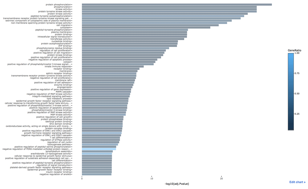

Figure 1. Based on 100 proteins most closely related to the RAS signaling pathway, top 75 categories from the ORA and their adjusted p-values, with the proportion of corresponding genes in a certain functional category of gene ontology.

The online version of this figure is interactive.

In GSEA, the gene list is sorted by the standardized score showing how much they are functionally close to the target. Genes with higher scores are functionally more related to the target. The positive values of the enrichment score indicate enrichment at the top of the ranked gene list. Thus proteins that closely related to the target are enriched in categories with high enrichment scores. In other words, these proteins are depleted in categories with low enrichment scores. We can see the RTK, MAPK and WNT signaling pathways in Figure 2. One possible reason is that AKT can activate β-catenin both indirectly and indirectly.

# gene sets for GO and KEGG pathway
library(KEGG.db)
pathway.id <- unique(kegg.mmu[,2])
yy <- split(kegg.mmu[,1], list(kegg.mmu$PathwayID))
library(Category)
names(yy) <- getPathNames(sub("[[:alpha:]]+....", "", pathway.id))
yy[which(names(yy) == "NA")] <- NULL

# remove duplicate categories
yy[intersect(names(xx), names(yy))] <- NULL

# GSEA
set.seed(1)
GSEAsummary <- fgsea(c(xx, yy), scaled.scores, nperm = 1000)
index <- which(GSEAsummary[,1] == names(yy[1]))
groups <- 0
groups[1:(index-1)] <- "GO"
groups[index:nrow(GSEAsummary)] <- "KEGG"
index <- match(data.frame(GSEAsummary[,1])[,1], names(c(xx, yy)))

# network visualization
g <- enrich.net(GSEAsummary, c(xx, yy)[index], node.id = "pathway", numChar = 100,
   pvalue = "pval", edge.cutoff = 0.2, pvalue.cutoff = 0.05, degree.cutoff = 1,
   n = 200, group = groups, vertex.label.cex = 0.6, vertex.label.color = "black")

# interactive figure
vs <- V(g)
es <- as.data.frame(get.edgelist(g))
Nv <- length(vs)
Ne <- length(es[1]$V1)

# create nodes
L <- layout.kamada.kawai(g)
Xn <- L[,1]
Yn <- L[,2]
group <- ifelse(V(g)$shape == "circle", "GO", "KEGG")
network <- plot_ly(x = ~Xn, y = ~Yn, type = "scatter", mode = "markers",
   marker = list(color = V(g)$color, size = V(g)$size*2,
      symbol= ~V(g)$shape, line = list(color = "gray", width = 2)),
   hoverinfo = "text", text = ~paste("</br>", group, "</br>", names(vs))) %>%
      add_annotations( x = ~Xn, y = ~Yn, text = names(vs), showarrow = FALSE,
   font = list(color = "gray", size = 10))

# create edges
edge_shapes <- list()
for(i in 1:Ne)
{
  v0 <- es[i,]$V1
  v1 <- es[i,]$V2
  index0 <- match(v0, names(V(g)))
  index1 <- match(v1, names(V(g)))
  edge_shape <- list(type = "line", line = list(color = "#030303",
     width = E(g)$width[i]), x0 = Xn[index0], y0 = Yn[index0],
     x1 = Xn[index1], y1 = Yn[index1])
  edge_shapes[[i]] <- edge_shape
}

# create network
axis <- list(title = "", showgrid = FALSE, showticklabels = FALSE, zeroline = FALSE)
h <- layout(network, title = "Enrichment Network", shapes = edge_shapes,
   xaxis = axis, yaxis = axis)
config(h, showLink = TRUE)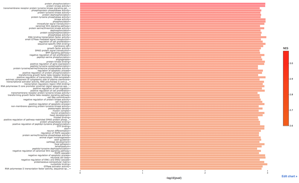

Figure 2. Top 75 categories and their p-values from the GSEA with scaled scores of genes from the target, RAS signaling pathway.

The online version of this figure is interactive.

In Figure 3, the network visualization of the functional enrichment analysis is displayed to minimize the effect of redundancy of gene sets and help in interpretation of enrichment analysis. Nodes indicate gene sets defined by GO terms or KEGG pathways. The connection between two nodes depends on the proportion of overlapping genes of corresponding two gene sets²¹. The size of nodes is proportional to the number of genes in their categories. The more significant categories are, the less transparent their nodes are. This network may be useful to produce more concise results of the functional enrichment. For GO terms, the two largest subnetworks are involved in transcription and signal transduction. We can see that RAS is related to tumorigenesis via the PI3K-AKT pathway from KEGG.

# top 20 proteins and 30 KEGG pathways
top.genes <- genes[1:20]
filtered.yy <- lapply(yy, intersect, top.genes)
filtered.yy <- filtered.yy[order(lengths(filtered.yy), decreasing = TRUE)[1:30]]

# matrix for heatmap
f <- function(x)
{
   index <- match(top.genes, rbind(x))
   rbind(x)[index]
}
mat <- ifelse(!is.na(t(sapply(filtered.yy, f))) == TRUE, 1, 0)

# find gene symbol
ensembl <- useMart("ensembl")
mouse.ensembl <- useDataset("mmusculus_gene_ensembl", mart = ensembl)
gene.name <- getBM(attributes = c("mgi_symbol", "entrezgene"), filters = "entrezgene",
   values = top.genes, mart = mouse.ensembl)
colnames(mat) <- gene.name[match(top.genes, gene.name[,2]), 1]

# heatmap
library(reshape2)
melt.mat <- melt(mat[c(nrow(mat):1),])
colnames(melt.mat) <- c("pathway", "gene", "value")
p <- ggplot(melt.mat, aes(gene, pathway)) +
   geom_tile(aes(fill = value), colour = "white") +
   scale_fill_gradient(low = "white", high = "black") +
   theme(legend.position = "none", axis.title.y = element_blank(),
      axis.text.x = element_text(angle = 90, hjust = 1))
 
# interactive figure
config(ggplotly(p), showLink = TRUE)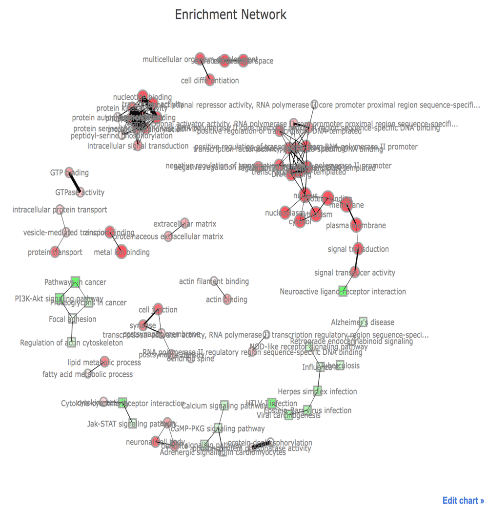

Figure 3. By using the 200 most significant categories from the GSEA, network visualization with GO in red and KEGG pathway in green, with the cutoff of 0.05 and 0.2 for p-values and edges, respectively.

The online version of this figure is interactive.

The binary heatmap for the relationship between top 20 proteins and 30 pathways is shown in Figure 4. The functionally related proteins mainly consist of ErbB receptors and adaptors. Also, they have PI3K and RAF proteins that can be activated by the RAS protein. Pathways containing these proteins are related to known biological functions. However, some of top proteins do not belong to these pathways.

# STRING
string_db <- STRINGdb$new(version = "10", species = 10090, score_threshold = 700)
target <- data.frame(path.04014)
top <- data.frame(top.genes)
names(top) <- "gene.id"

# mapping
string_db.map.target <- string_db$map(target, "path.04014", removeUnmappedRows = TRUE)
string_db.map.top <- string_db$map(top, "gene.id", removeUnmappedRows = TRUE)
target <- string_db.map.target$STRING_id
top.proteins <- string_db.map.top$STRING_id

# PPI visualization
payload_id <- string_db$post_payload(c(target, top.proteins),
   colors = c(rep("#00ff00", length(target)), rep("#ff0000", length(top.proteins))))
string_db$plot_network(c(target, top.proteins), payload_id = payload_id)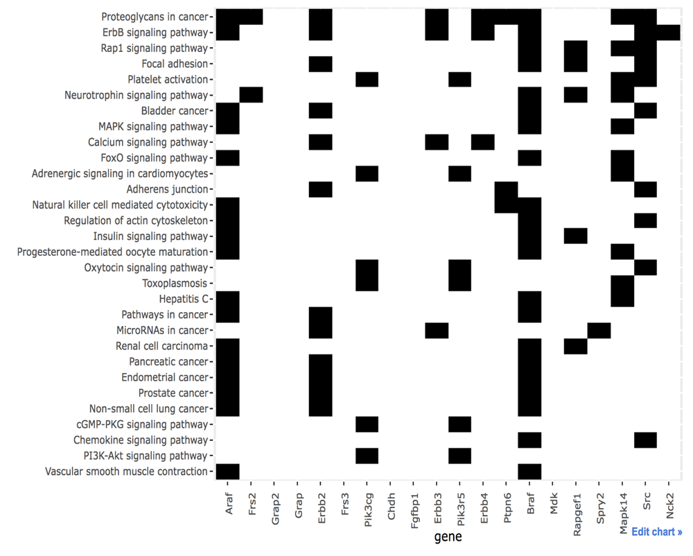

Figure 4. Relationship between KEGG pathways and the corresponding genes of the top 20 proteins.

The online version of this figure is interactive.

In Figure 5, the network for high-confidence protein interactions of the RAS pathway and top 20 proteins is drawn by STRING. As expected, top 20 proteins are connected to the target proteins. We can find several types of interactions from the legend of STRING database, but not shown here. For example, interactions between FGFBP1 and the RAS pathway are experimentally determined. On the other hand, interactions with CHDH come from curated databases. CHDH regulated by estrogen in breast cancer is connected to the PLA2 family of the RAS pathway. Also, it is known that PLA2 is phosphorylated by MAPK. Thus the association between CHDH and the RAS pathway is reasonable. Therefore, this approach may be helpful to explain how cytoplasmic mitogenic signaling cascades are activated by estrogen and understand the role of estrogen in breast cancer.

# adjacency matrix
string_db.graph <- string_db$get_graph()
string_db.adjacency <- as_adjacency_matrix(string_db.graph, type = "both")
rownames(string_db.adjacency) <- sub(".*\\.", "", rownames(string_db.adjacency))
colnames(string_db.adjacency) <- sub(".*\\.", "", colnames(string_db.adjacency))

# proteins of RAS pathway
path.04014.protein <- getBM(attributes = "ensembl_peptide_id", filters = "entrezgene",
   values = path.04014, mart = mouse.ensembl)[,1]
path.04014.protein <- intersect(path.04014.protein, rownames(string_db.adjacency))

# first level neighbors of a set of proteins of RAS pathway
string_db.adjacency.path.04014 <- string_db.adjacency[path.04014.protein,]
index <- which(colSums(as.matrix(string_db.adjacency.path.04014)) > 0)
first.nb.protein <- colnames(string_db.adjacency.path.04014)[index]
first.nb.protein <- setdiff(first.nb.protein, path.04014.protein)

# first level neighbors of a set of genes of RAS pathway
first.nb.gene <- getBM(attributes = "entrezgene", filters = "ensembl_peptide_id",
   values = first.nb.protein, mart = mouse.ensembl)[,1]
first.nb.gene <- intersect(first.nb.gene, genes)

# bootstrap
library(boot)
num.overlap <- function(x, index)
{
length(intersect(x[index][1:20], first.nb.gene))
}

# observed value
length(intersect(top.genes, first.nb.gene))

# resampling
set.seed(1)
(boot.obj <- boot(genes, num.overlap, R = 10000))
boot.num.overlap <- data.frame(boot.obj$t)
colnames(boot.num.overlap) <- "num.overlap.gene"
p <- ggplot(boot.num.overlap, aes(num.overlap.gene)) +
   geom_histogram(stat = "bin", binwidth = 0.5) +
   labs(x = "Number of overlapping genes", y = "Count") +
   scale_x_continuous(breaks = pretty(boot.num.overlap$num.overlap.gene,
     n = length(unique(boot.num.overlap$num.overlap.gene)))) +
   theme_bw() +
   theme(axis.line = element_line(colour = "black"),
     panel.grid.major = element_blank(),
     panel.grid.minor = element_blank(),
     panel.border = element_blank(),
     panel.background = element_blank(),
     plot.margin = margin(0, 0, 10, 20))

# interactive figure
config(ggplotly(p), showLink = TRUE)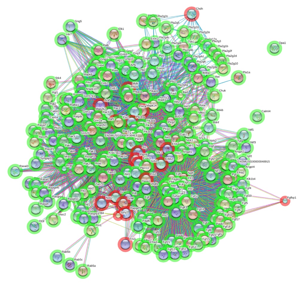

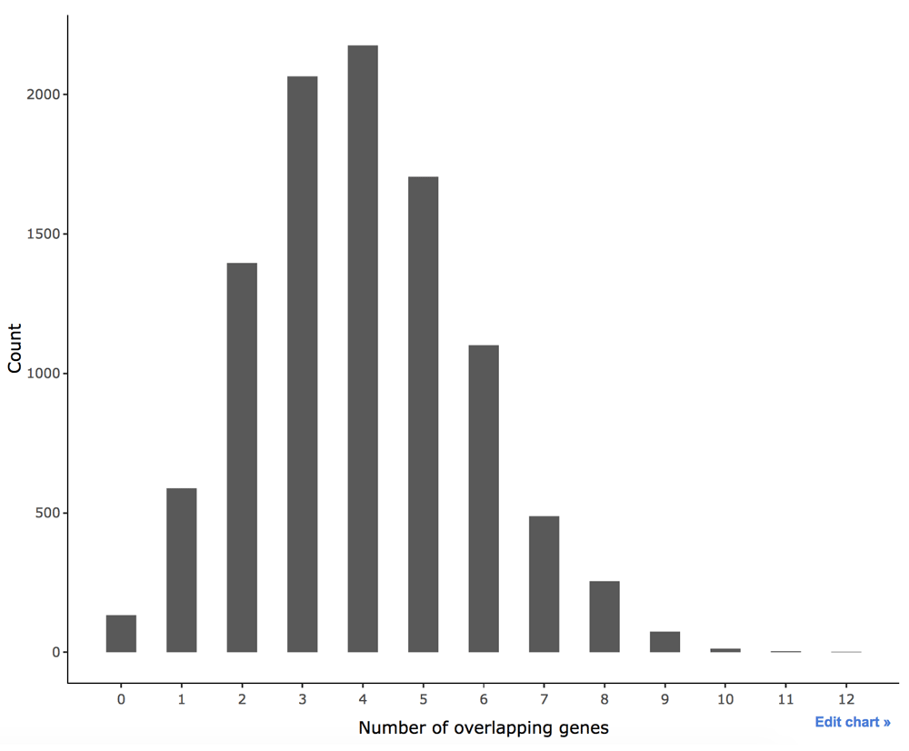
Figure 5. PPI and gene symbols of the top 20 proteins with a red halo and the RAS pathway with a green halo.

We observe that top 20 proteins are connected to the proteins of the RAS pathway. Similarly, the corresponding genes of the top 20 proteins are connected to those of the target proteins. The first level neighbors of the RAS pathway can be assumed as genes that are connected to the pathway but not chosen by the algorithm. Consider the number of overlapping genes between the first level neighbors and randomly selected 20 genes. Thus, the overlapping genes are randomly selected genes connected to the RAS pathway. The bootstrap method can be used to estimate the distribution of the number of overlapping genes. In Figure 6, the statistic ranges from 0 to 12, based on 10,000 bootstrap replicates. We can conclude that the number of connected genes obtained from the original data is significantly greater than what could be obtained by chance. Therefore, this algorithm seems to be good enough to infer functionally related proteins.

Figure 6. Distribution of number of overlapping genes between the first level neighbors of the RAS pathway and randomly selected 20 genes by using the bootstrap method.

The online version of this figure is interactive.

Discussion

The proposed method is highly dependent on protein interaction networks. There are many databases of protein interactions with millions of predicted protein interactions as well we interactions reported in thousands of publications. Therefore, the choice of data can be critical. Also, the one-class support vector machine can be sensitive to changes in parameters. Although the classical support vector machine has good performance, overall performance may be dominated by the OCSVM since the OCSVM is followed by the SVM. However, it would be worthwhile to provide potential to infer the putative functions of proteins from PPI by complementing conventional methods based on protein sequence analyses.

Data availability

The PPInfer package is available at: http://bioconductor.org/packages/PPInfer/

Source code is available at: https://github.com/dongminjung/PPInfer

Archived source code as at the time of publication: https://doi.org/doi:10.5281/zenodo.1035128

License: Artistic-2.0

Competing interests

No competing interests were disclosed.

Grant information

This material is based upon work supported by the National Science Foundation/EPSCoR Grant Number IIA-1355423 and by the State of South Dakota. Any opinions, findings, and conclusions or recommendations expressed in this material are those of the author(s) and do not necessarily reflect the views of the National Science Foundation.

The funders had no role in study design, data collection and analysis, decision to publish, or preparation of the manuscript.

Faculty Opinions recommended

References

1. Chatr-Aryamontri A, Breitkreutz BJ, Heinicke S, et al.: The BioGRID interaction database: 2013 update. Nucleic Acids Res. 2013; 41(Database issue): D816–D823. PubMed Abstract | Publisher Full Text | Free Full Text
2. Szklarczyk D, Franceschini A, Wyder S, et al.: STRING v10: protein-protein interaction networks, integrated over the tree of life. Nucleic Acids Res. 2015; 43(Database issue): D447–52. PubMed Abstract | Publisher Full Text | Free Full Text
3. Fellenberg M, Albermann K, Zollner A, et al.: Integrative analysis of protein interaction data. Proc Int Conf Intell Syst Mol Biol. 2000; 8: 152–161. PubMed Abstract
4. Schwikowski B, Uetz P, Fields S: A network of protein-protein interactions in yeast. Nat Biotechnol. 2000; 18(12): 1257–1261. PubMed Abstract | Publisher Full Text
5. Deng M, Zhang K, Mehta S, et al.: Prediction of protein function using protein-protein interaction data. J Comput Biol. 2003; 10(6): 947–960. PubMed Abstract | Publisher Full Text
6. Deng M, Chen T, Sun F: An integrated probabilistic model for functional prediction of proteins. J Comput Biol. 2004; 11(2–3): 463–475. PubMed Abstract | Publisher Full Text
7. Joshi T, Chen Y, Becker JM, et al.: Genome-scale gene function prediction using multiple sources of high-throughput data in yeast Saccharomyces cerevisiae. OMICS. 2004; 8(4): 322–333. PubMed Abstract | Publisher Full Text
8. Peng W, Wang J, Cai J, et al.: Improving protein function prediction using domain and protein complexes in PPI networks. BMC Syst Biol. 2014; 8(1): 35. PubMed Abstract | Publisher Full Text | Free Full Text
9. Vapnik V: The nature of statistical learning theory. Springer-Verlag. 1995. Publisher Full Text
10. Cover TM: Geometrical and statistical properties of systems of linear inequalities with applications in pattern recognition. IEEE Transactions on Electronic Computers. 1965; EC-14(3): 326–334. Publisher Full Text
11. Kondor R, Lafferty J: Diffusion kernels on graphs and other discrete structures. In Proceedings of the 19th International Conference on Machine Learning. 2002; 315–322. Reference Source
12. Cook DJ, Holder LB (Eds.): Mining graph data. John Wiley & Sons. 2006. Publisher Full Text
13. Smola AJ, Kondor R: Kernels and regularization on graphs. In Learning theory and kernel machines. Springer. 2003; 144–158. Publisher Full Text
14. Samatova NF, Hendrix W, Jenkins J, et al.(Eds.): Practical graph mining with R. CRC Press. 2013. Reference Source
15. Kolaczyk ED, Csardi G: Statistical analysis of network data with R. Springer. 2014. Publisher Full Text
16. Scholkopf B, Burges CJ, Smola AJ: Advances in kernel methods: support vector learning. MIT press. 1999. Reference Source
17. Ma Y, Guo G: Support vector machines applications. Springer. 2014. Publisher Full Text
18. Abe S: Support vector machines for pattern classification. Springer. 2010. Publisher Full Text
19. Tax DM, Duin RP: Support vector data description. Mach Learn. 2004; 54(1): 45–66. Publisher Full Text
20. Senay SD, Worner SP, Ikeda T: Novel three-step pseudo-absence selection technique for improved species distribution modelling. PLoS One. 2013; 8(8): e71218. PubMed Abstract | Publisher Full Text | Free Full Text
21. Yu G, Wang LG, Yan GR, et al.: DOSE: an R/Bioconductor package for disease ontology semantic and enrichment analysis. Bioinformatics. 2014; 31(4): 608–609. PubMed Abstract | Publisher Full Text

Comments on this article Comments (0)

Version 3

VERSION 3 PUBLISHED 07 Nov 2017

Author details Author details

¹ Avison Biomedical Research Center, Yonsei University, Seoul, South Korea
² Department of Mathematics and Statistics, South Dakota State University, Brookings, SD, USA

Dongmin Jung
Roles: Conceptualization, Investigation, Methodology, Software, Visualization, Writing – Original Draft Preparation

Xijin Ge
Roles: Conceptualization, Funding Acquisition, Investigation, Methodology, Validation, Visualization, Writing – Review & Editing

Competing interests

No competing interests were disclosed.

Grant information

This material is based upon work supported by the National Science Foundation/EPSCoR Grant Number IIA-1355423 and by the State of South Dakota
The funders had no role in study design, data collection and analysis, decision to publish, or preparation of the manuscript.

Article Versions (3)

version 3

Revised

Published: 12 Mar 2018, 6:1969

https://doi.org/10.12688/f1000research.12947.3

version 2

Revised

Published: 08 Dec 2017, 6:1969

https://doi.org/10.12688/f1000research.12947.2

version 1

Published: 07 Nov 2017, 6:1969

https://doi.org/10.12688/f1000research.12947.1

© 2018 Jung D and Ge X. This is an open access article distributed under the terms of the Creative Commons Attribution License, which permits unrestricted use, distribution, and reproduction in any medium, provided the original work is properly cited. Data associated with the article are available under the terms of the Creative Commons Zero "No rights reserved" data waiver (CC0 1.0 Public domain dedication).

Download

Export To

metrics

	Views	Downloads
F1000Research	-	-
PubMed Central Data from PMC are received and updated monthly.	-	-

Citations

SEE MORE DETAILS

CITE

how to cite this article

Jung D and Ge X. PPInfer: a Bioconductor package for inferring functionally related proteins using protein interaction networks [version 3; peer review: 1 approved, 1 approved with reservations]. F1000Research 2018, 6:1969 (https://doi.org/10.12688/f1000research.12947.3)

NOTE: If applicable, it is important to ensure the information in square brackets after the title is included in all citations of this article.

track

receive updates on this article

Track an article to receive email alerts on any updates to this article.

Open Peer Review

Version 3

VERSION 3

PUBLISHED 12 Mar 2018

Revised

Views

Reviewer Report 13 Mar 2018

Helen V. Cook, Novo Nordisk Foundation Center for Protein Research, Faculty of Health and Medical Sciences, University of Copenhagen, Copenhagen, Denmark

Approved with Reservations

https://doi.org/10.5256/f1000research.15364.r31789

Thank you for providing answers to my specific questions, and for the detailed description of the method. This clears up several matters.

The addition of Figure 6 is helpful. You may additionally want to calculate a p-value to highlight how unexpected your result is compared to the distribution generated from bootstrapping.

However, I still have some reservations about the evaluation of the results.

The method described in the paper returns a set of proteins that are similar in function to a target set. The way I would expect to see this evaluated is to compare the results for the RAS pathway against a gold standard set which would be determined beforehand and would include all and only the proteins that should be annotated the same as the RAS pathway. The paper should justify how this gold standard was determined, whether it was hand annotated or otherwise. I would then expect to see the recall and precision of the method calculated against this gold standard, along with an error analysis to show what types of proteins are false positives and negatives, and to discuss why these proteins are returned/missed. Sorry for not making this clearer in the original report, but this is what I intended by questions 5-7. The discussion of the results shown in Figures 1-4 centres on the true positives, but it is discussion and quantification of the false positives and false negatives that will provide credibility to your method. As it stands now, the evaluation that is provided in the paper is not sufficient for me to feel comfortable about using the results for a biological analysis.

Competing Interests: No competing interests were disclosed.

I confirm that I have read this submission and believe that I have an appropriate level of expertise to confirm that it is of an acceptable scientific standard, however I have significant reservations, as outlined above.

CITE

Report a concern

Respond or Comment

Version 2

VERSION 2

PUBLISHED 08 Dec 2017

Revised

Views

Reviewer Report 25 Jan 2018

Helen V. Cook, Novo Nordisk Foundation Center for Protein Research, Faculty of Health and Medical Sciences, University of Copenhagen, Copenhagen, Denmark

Approved with Reservations

https://doi.org/10.5256/f1000research.14483.r30170

The question of how to predict functions for proteins with unknown function is interesting and highly relevant to biology. Using a machine learning strategy, as is done in this work, is a reasonable way to approach this task.

This paper by Jung and Ge presents a method to assign functions to proteins along with code which is available on github and installable via bioconductor. Thank you for making your code open source and easily available to install and use.

I was able to run the R code and reproduce the figures in the paper following the given use case and using the comment left by the previous reviewers. However, the methods section in the paper does not provide sufficient details for me to recreate the software. Much of what is written in the methods section is introduction to the methods, and describes in general how they work. It does not provide a detailed description of how these methods are applied to the problem the authors are trying to solve. Even though the code is provided, the application of the methods must be described in detail in the paper. Further, the R package includes the pre-trained (extremely large, 3Gb) model and neither the code nor the paper includes details on how to reproduce the model, or how to train it again on new data. Specifically, the following questions must be clearly answered, and a figure to illustrate the method would be a helpful addition.

What are the features provided to the OCSVM, and what is the output?
What are the features provided to the subsequent SVM, and what is the output?
How was a gold standard set of annotations (for each organism) selected?
On what data was the model trained and how can the model be reproduced?
How was the data partitioned for training, testing and evaluation of the SVM?
What is the performance of the two SVMs on their respective test sets?
What evaluation methods do the authors use ensure that their models are not overfit?
What parameters were used for each SVM, and how/why were they selected?

The use case predicts mouse proteins that have similar function to the Ras signalling pathway as defined by KEGG. Figures 1 through 4 present different ways of visualizing the GO terms and KEGG pathways that the predicted proteins are related to. GO terms such as "kinase activity" are significantly overrepresented in these proteins, which is confusing since the Ras pathway signals via GTPases, not kinases. Figure 5 shows a STRING network of the proteins in the Ras pathway, together with the top 20 predicted proteins. The authors claim that because there are STRING interactions between these two sets of proteins that this is support for them having the same function. To support this, I would at least like to see this number of interactions compared to those between a random set of 20 proteins and the proteins of the Ras pathway, if not additionally some error analysis of proteins that are also connected to the pathway but not picked by the algorithm. It is also not clear to me if the training data for the SVMs make use of the network interactions; if it does, then providing STRING interactions as support for validating the output is circular.

Since the paper leaves open some fundamental questions in the design of the machine learning approach, I cannot approve this article without major reservations. I hope that the authors will add these additional details, since this article addresses an interesting problem, and I am curious to see their method described in detail.

Some minor comments on the article follow:

All acronyms such as ORA should be defined in the text.
The Figure 1 generated by the example code is not exactly the same as the plot included in the manuscript, but is very close. The figure caption for Figure 1 should specify what the size of the points means.
I cannot replicate Figure 2 with the code provided, but it seems that the underlying data is the same as the published figure.
The package PPInfer should depend on limma, KEGG.db and GO.db since these are necessary to run the use case.
The text for the interactive figures is too large, making them very difficult to read - although it is not clear to me if this is a bug in the F1000Research website itself or in the underlying figure.

Is the rationale for developing the new software tool clearly explained?

Yes
Is the description of the software tool technically sound?

No
Are sufficient details of the code, methods and analysis (if applicable) provided to allow replication of the software development and its use by others?

No
Is sufficient information provided to allow interpretation of the expected output datasets and any results generated using the tool?

Partly
Are the conclusions about the tool and its performance adequately supported by the findings presented in the article?

Partly

Competing Interests: No competing interests were disclosed.

CITE

Report a concern

Author Response 12 Mar 2018

Dongmin Jung, Avison Biomedical Research Center, Yonsei University, Seoul, South Korea

12 Mar 2018

Author Response

Thank you for taking the time to read and review our paper. In the revised version, we have updated the figures and the text in several places, according to your ... Continue reading Thank you for taking the time to read and review our paper. In the revised version, we have updated the figures and the text in several places, according to your comment.

1. What are the features provided to the OCSVM, and what is the output?
The regularized Laplacian matrix for the whole graph is used as input for the OCSVM. Nodes in the one class are used for training. Unlabeled nodes are scored as output. Please, see the text for detailed explanation.

2. What are the features provided to the subsequent SVM, and what is the output?
The regularized Laplacian matrix is used as input for the SVM. Nodes in the two classes are used for training. Unlabeled nodes are scored as output.

3. How was a gold standard set of annotations (for each organism) selected?
Although various functional annotations could be used to categorize genes, gene ontology probably the most widely used function categorization. KEGG is one of the most widely used categorization in pathway analysis. Also, they provide annotations of diverse organisms. This is why we choose GO and KEGG for annotation.

4. On what data was the model trained and how can the model be reproduced?
The uploaded kernel matrix is not the pre-trained model but the regularized Laplacian matrix used for the kernel for SVMs. This kernel matrix can be obtained for mouse as follows.
string.db.10090 <- STRINGdb$new(version='10', species = 10090)
string.db.10090.graph <- string.db.10090$get_graph()
K.10090 <- net.kernel(string.db.10090.graph)

5. How was the data partitioned for training, testing and evaluation of the SVM?
Nodes with the class label are used for training. Unlabeled nodes are predicted. Evaluation can be performed by using the option 'cross' in the function 'ppi.infer.mouse'. For example, 'cross = 10' for 10-fold cross-validation.

6. What is the performance of the two SVMs on their respective test sets?
As we discussed, the OCSVM can be sensitive to the choice of kernels and parameters. Although the classical SVM has good performance, overall performance may be dominated by the OCSVM since the OCSVM is followed by the SVM.

7. What evaluation methods do the authors use ensure that their models are not overfit?
We have the option for the k-fold cross validation to check whether models are overfit or not.

8. What parameters were used for each SVM, and how/why were they selected?
The parameter for misclassification cost is used for the SVM. This is a constant of the regularization term in the Lagrangian function. Similarly, the 'nu' parameter about a regularization for a hypersphere is needed for the OCSVM. Also, the parameter for convergence is used for both models. In this example, we used default parameters of the function 'ksvm' in the package 'kernlab'. These parameters are set as default in this package.

For the results of functional enrichment analysis, categories related to GTPase activity may not be shown in figures. Since some part of results is just reported due to limited space, you can see such categories in the full list of significant categories. Also, the result may not be exactly reproducible because functional categories are frequently updated and there still exists randomness in the function 'fgsea' even setting a seed. Finally, the number of interactions we obtained is compared to those between a random set of 20 proteins and the proteins of the RAS pathway by using bootstrapping. Please, see the text and figure for further discussion.
Thank you for taking the time to read and review our paper. In the revised version, we have updated the figures and the text in several places, according to your comment.

1. What are the features provided to the OCSVM, and what is the output?
The regularized Laplacian matrix for the whole graph is used as input for the OCSVM. Nodes in the one class are used for training. Unlabeled nodes are scored as output. Please, see the text for detailed explanation.

2. What are the features provided to the subsequent SVM, and what is the output?
The regularized Laplacian matrix is used as input for the SVM. Nodes in the two classes are used for training. Unlabeled nodes are scored as output.

3. How was a gold standard set of annotations (for each organism) selected?
Although various functional annotations could be used to categorize genes, gene ontology probably the most widely used function categorization. KEGG is one of the most widely used categorization in pathway analysis. Also, they provide annotations of diverse organisms. This is why we choose GO and KEGG for annotation.

4. On what data was the model trained and how can the model be reproduced?
The uploaded kernel matrix is not the pre-trained model but the regularized Laplacian matrix used for the kernel for SVMs. This kernel matrix can be obtained for mouse as follows.
string.db.10090 <- STRINGdb$new(version='10', species = 10090)
string.db.10090.graph <- string.db.10090$get_graph()
K.10090 <- net.kernel(string.db.10090.graph)

5. How was the data partitioned for training, testing and evaluation of the SVM?
Nodes with the class label are used for training. Unlabeled nodes are predicted. Evaluation can be performed by using the option 'cross' in the function 'ppi.infer.mouse'. For example, 'cross = 10' for 10-fold cross-validation.

6. What is the performance of the two SVMs on their respective test sets?
As we discussed, the OCSVM can be sensitive to the choice of kernels and parameters. Although the classical SVM has good performance, overall performance may be dominated by the OCSVM since the OCSVM is followed by the SVM.

7. What evaluation methods do the authors use ensure that their models are not overfit?
We have the option for the k-fold cross validation to check whether models are overfit or not.

8. What parameters were used for each SVM, and how/why were they selected?
The parameter for misclassification cost is used for the SVM. This is a constant of the regularization term in the Lagrangian function. Similarly, the 'nu' parameter about a regularization for a hypersphere is needed for the OCSVM. Also, the parameter for convergence is used for both models. In this example, we used default parameters of the function 'ksvm' in the package 'kernlab'. These parameters are set as default in this package.

For the results of functional enrichment analysis, categories related to GTPase activity may not be shown in figures. Since some part of results is just reported due to limited space, you can see such categories in the full list of significant categories. Also, the result may not be exactly reproducible because functional categories are frequently updated and there still exists randomness in the function 'fgsea' even setting a seed. Finally, the number of interactions we obtained is compared to those between a random set of 20 proteins and the proteins of the RAS pathway by using bootstrapping. Please, see the text and figure for further discussion.
Competing Interests: No competing interests were disclosed. Close
Report a concern
Respond or Comment

COMMENTS ON THIS REPORT

Author Response 12 Mar 2018

Dongmin Jung, Avison Biomedical Research Center, Yonsei University, Seoul, South Korea

12 Mar 2018

Author Response

Thank you for taking the time to read and review our paper. In the revised version, we have updated the figures and the text in several places, according to your ... Continue reading Thank you for taking the time to read and review our paper. In the revised version, we have updated the figures and the text in several places, according to your comment.

1. What are the features provided to the OCSVM, and what is the output?
The regularized Laplacian matrix for the whole graph is used as input for the OCSVM. Nodes in the one class are used for training. Unlabeled nodes are scored as output. Please, see the text for detailed explanation.

2. What are the features provided to the subsequent SVM, and what is the output?
The regularized Laplacian matrix is used as input for the SVM. Nodes in the two classes are used for training. Unlabeled nodes are scored as output.

3. How was a gold standard set of annotations (for each organism) selected?
Although various functional annotations could be used to categorize genes, gene ontology probably the most widely used function categorization. KEGG is one of the most widely used categorization in pathway analysis. Also, they provide annotations of diverse organisms. This is why we choose GO and KEGG for annotation.

4. On what data was the model trained and how can the model be reproduced?
The uploaded kernel matrix is not the pre-trained model but the regularized Laplacian matrix used for the kernel for SVMs. This kernel matrix can be obtained for mouse as follows.
string.db.10090 <- STRINGdb$new(version='10', species = 10090)
string.db.10090.graph <- string.db.10090$get_graph()
K.10090 <- net.kernel(string.db.10090.graph)

5. How was the data partitioned for training, testing and evaluation of the SVM?
Nodes with the class label are used for training. Unlabeled nodes are predicted. Evaluation can be performed by using the option 'cross' in the function 'ppi.infer.mouse'. For example, 'cross = 10' for 10-fold cross-validation.

6. What is the performance of the two SVMs on their respective test sets?
As we discussed, the OCSVM can be sensitive to the choice of kernels and parameters. Although the classical SVM has good performance, overall performance may be dominated by the OCSVM since the OCSVM is followed by the SVM.

7. What evaluation methods do the authors use ensure that their models are not overfit?
We have the option for the k-fold cross validation to check whether models are overfit or not.

8. What parameters were used for each SVM, and how/why were they selected?
The parameter for misclassification cost is used for the SVM. This is a constant of the regularization term in the Lagrangian function. Similarly, the 'nu' parameter about a regularization for a hypersphere is needed for the OCSVM. Also, the parameter for convergence is used for both models. In this example, we used default parameters of the function 'ksvm' in the package 'kernlab'. These parameters are set as default in this package.

For the results of functional enrichment analysis, categories related to GTPase activity may not be shown in figures. Since some part of results is just reported due to limited space, you can see such categories in the full list of significant categories. Also, the result may not be exactly reproducible because functional categories are frequently updated and there still exists randomness in the function 'fgsea' even setting a seed. Finally, the number of interactions we obtained is compared to those between a random set of 20 proteins and the proteins of the RAS pathway by using bootstrapping. Please, see the text and figure for further discussion.
Thank you for taking the time to read and review our paper. In the revised version, we have updated the figures and the text in several places, according to your comment.

1. What are the features provided to the OCSVM, and what is the output?
The regularized Laplacian matrix for the whole graph is used as input for the OCSVM. Nodes in the one class are used for training. Unlabeled nodes are scored as output. Please, see the text for detailed explanation.

2. What are the features provided to the subsequent SVM, and what is the output?
The regularized Laplacian matrix is used as input for the SVM. Nodes in the two classes are used for training. Unlabeled nodes are scored as output.

3. How was a gold standard set of annotations (for each organism) selected?
Although various functional annotations could be used to categorize genes, gene ontology probably the most widely used function categorization. KEGG is one of the most widely used categorization in pathway analysis. Also, they provide annotations of diverse organisms. This is why we choose GO and KEGG for annotation.

4. On what data was the model trained and how can the model be reproduced?
The uploaded kernel matrix is not the pre-trained model but the regularized Laplacian matrix used for the kernel for SVMs. This kernel matrix can be obtained for mouse as follows.
string.db.10090 <- STRINGdb$new(version='10', species = 10090)
string.db.10090.graph <- string.db.10090$get_graph()
K.10090 <- net.kernel(string.db.10090.graph)

5. How was the data partitioned for training, testing and evaluation of the SVM?
Nodes with the class label are used for training. Unlabeled nodes are predicted. Evaluation can be performed by using the option 'cross' in the function 'ppi.infer.mouse'. For example, 'cross = 10' for 10-fold cross-validation.

6. What is the performance of the two SVMs on their respective test sets?
As we discussed, the OCSVM can be sensitive to the choice of kernels and parameters. Although the classical SVM has good performance, overall performance may be dominated by the OCSVM since the OCSVM is followed by the SVM.

7. What evaluation methods do the authors use ensure that their models are not overfit?
We have the option for the k-fold cross validation to check whether models are overfit or not.

8. What parameters were used for each SVM, and how/why were they selected?
The parameter for misclassification cost is used for the SVM. This is a constant of the regularization term in the Lagrangian function. Similarly, the 'nu' parameter about a regularization for a hypersphere is needed for the OCSVM. Also, the parameter for convergence is used for both models. In this example, we used default parameters of the function 'ksvm' in the package 'kernlab'. These parameters are set as default in this package.

For the results of functional enrichment analysis, categories related to GTPase activity may not be shown in figures. Since some part of results is just reported due to limited space, you can see such categories in the full list of significant categories. Also, the result may not be exactly reproducible because functional categories are frequently updated and there still exists randomness in the function 'fgsea' even setting a seed. Finally, the number of interactions we obtained is compared to those between a random set of 20 proteins and the proteins of the RAS pathway by using bootstrapping. Please, see the text and figure for further discussion.
Competing Interests: No competing interests were disclosed. Close
Report a concern

Views

Reviewer Report 11 Dec 2017

Cathy H. Wu, Center for Bioinformatics & Computational Biology (CBCB), University of Delaware, Newark, DE, USA

Karen E. Ross, Department of Biochemistry and Molecular & Cellular Biology, Georgetown University Medical Center, Washington, DC, USA

Approved

https://doi.org/10.5256/f1000research.14483.r28845

CITE

Report a concern

Respond or Comment

Version 1

VERSION 1

PUBLISHED 07 Nov 2017

Views

Reviewer Report 22 Nov 2017

Cathy H. Wu, Center for Bioinformatics & Computational Biology (CBCB), University of Delaware, Newark, DE, USA

Karen E. Ross, Department of Biochemistry and Molecular & Cellular Biology, Georgetown University Medical Center, Washington, DC, USA

Approved with Reservations

https://doi.org/10.5256/f1000research.14038.r27695

The article describes a new R package, PPInfer, for inferring functions of proteins based on their connectivity in a PPI network. Discovery of new functions for proteins is an important problem and the method as described is an interesting and theoretically sound approach.

The authors provide detailed example code for using PPInfer. Unfortunately, when trying to reproduce the use case, there was an error in the first step:

> K.10090 <- readRDS("K10090.rds")
Error in gzfile(file, "rb") : cannot open the connection
In addition: Warning message:
In gzfile(file, "rb") :
cannot open compressed file 'K10090.rds', probable reason 'No such file or directory'

Therefore, we couldn't test the rest of the use case.

Also, in general, the use case would benefit from more text explanation so that readers understand the purpose of the tool and how to interpret the results. Specifically:

What is the meaning of the gene ratio on the x-axis in Figure 1?
In Figure 3, are the nodes enriched KEGG pathways and GO terms as determined by GSEA? What was the threshold for deciding which nodes should appear in the graph? What is the biological message of this graph?
A discussion of the functionally related proteins themselves (not just the enriched terms/pathways) would be helpful. How do these proteins functionally interact with the ras pathway proteins in the STRING network? Perhaps you could discuss the STRING confidence scores or types of evidence for these interactions.
It would be helpful to have more discussion of exactly what we learn from this approach. Can we infer that the proteins identified in the use case might be involved in the Ras pathway? It seems like based on the GO/KEGG annotation for the proteins, we could already have assumed they had something to do with signal transduction even without knowing that they are closely associated with Ras pathway proteins. Are there any examples of proteins whose association with the Ras pathway was surprising? Are there any proteins about which little is known or whose GO/KEGG annotation does not indiciate that they would be associated with the Ras pathway?

Please note that for questions 3, 4, and 5 on the referee report form: we were unable to fully evaluate this as we were unable to run the software. We have therefore assigned the answer "no" to reflect this.

Is the rationale for developing the new software tool clearly explained?

Partly
Is the description of the software tool technically sound?

Yes
Are sufficient details of the code, methods and analysis (if applicable) provided to allow replication of the software development and its use by others?

No
Is sufficient information provided to allow interpretation of the expected output datasets and any results generated using the tool?

No
Are the conclusions about the tool and its performance adequately supported by the findings presented in the article?

No

Competing Interests: No competing interests were disclosed.

We confirm that we have read this submission and believe that we have an appropriate level of expertise to confirm that it is of an acceptable scientific standard, however we have significant reservations, as outlined above.

CITE

Report a concern

Author Response 08 Dec 2017

Dongmin Jung, Avison Biomedical Research Center, Yonsei University, Seoul, South Korea

08 Dec 2017

Author Response

Thank you for taking the time to read and review our paper. In the revised version, we have improved the clarity of the figures and the text in several places, ... Continue reading Thank you for taking the time to read and review our paper. In the revised version, we have improved the clarity of the figures and the text in several places, according to your suggestions.

Necessary files are available at https://zenodo.org/record/1066236. Please, download K10090.rds and install the current version of this package.

In Figure 1, The horizontal axis represents the proportion of our interesting genes in a certain functional category.

In Figure 3, the 200 most significant categories from the GSEA are used, with the cutoff of 0.05 and 0.2 for p-values and edges, respectively. For GO terms, the two largest subnetworks are involved in transcription and signal transduction. We can see that Ras is related to tumorigenesis via the PI3K-Akt pathway from KEGG.

For the discussion of the functionally related proteins themselves, two figures are added. One is the heatmap for the relationship between top proteins and pathways in Figure 4. The other is visualization of PPI among proteins in Figure 5. Please, see the text for further discussion.

Thank you for taking the time to read and review our paper. In the revised version, we have improved the clarity of the figures and the text in several places, according to your suggestions.

Necessary files are available at https://zenodo.org/record/1066236. Please, download K10090.rds and install the current version of this package.

In Figure 1, The horizontal axis represents the proportion of our interesting genes in a certain functional category.

In Figure 3, the 200 most significant categories from the GSEA are used, with the cutoff of 0.05 and 0.2 for p-values and edges, respectively. For GO terms, the two largest subnetworks are involved in transcription and signal transduction. We can see that Ras is related to tumorigenesis via the PI3K-Akt pathway from KEGG.

For the discussion of the functionally related proteins themselves, two figures are added. One is the heatmap for the relationship between top proteins and pathways in Figure 4. The other is visualization of PPI among proteins in Figure 5. Please, see the text for further discussion.
Competing Interests: No competing interests were disclosed. Close
Report a concern
Respond or Comment

COMMENTS ON THIS REPORT

Author Response 08 Dec 2017

Dongmin Jung, Avison Biomedical Research Center, Yonsei University, Seoul, South Korea

08 Dec 2017

Author Response

Thank you for taking the time to read and review our paper. In the revised version, we have improved the clarity of the figures and the text in several places, ... Continue reading Thank you for taking the time to read and review our paper. In the revised version, we have improved the clarity of the figures and the text in several places, according to your suggestions.

Necessary files are available at https://zenodo.org/record/1066236. Please, download K10090.rds and install the current version of this package.

In Figure 1, The horizontal axis represents the proportion of our interesting genes in a certain functional category.

In Figure 3, the 200 most significant categories from the GSEA are used, with the cutoff of 0.05 and 0.2 for p-values and edges, respectively. For GO terms, the two largest subnetworks are involved in transcription and signal transduction. We can see that Ras is related to tumorigenesis via the PI3K-Akt pathway from KEGG.

For the discussion of the functionally related proteins themselves, two figures are added. One is the heatmap for the relationship between top proteins and pathways in Figure 4. The other is visualization of PPI among proteins in Figure 5. Please, see the text for further discussion.

Thank you for taking the time to read and review our paper. In the revised version, we have improved the clarity of the figures and the text in several places, according to your suggestions.

Necessary files are available at https://zenodo.org/record/1066236. Please, download K10090.rds and install the current version of this package.

In Figure 1, The horizontal axis represents the proportion of our interesting genes in a certain functional category.

In Figure 3, the 200 most significant categories from the GSEA are used, with the cutoff of 0.05 and 0.2 for p-values and edges, respectively. For GO terms, the two largest subnetworks are involved in transcription and signal transduction. We can see that Ras is related to tumorigenesis via the PI3K-Akt pathway from KEGG.

For the discussion of the functionally related proteins themselves, two figures are added. One is the heatmap for the relationship between top proteins and pathways in Figure 4. The other is visualization of PPI among proteins in Figure 5. Please, see the text for further discussion.
Competing Interests: No competing interests were disclosed. Close
Report a concern

Comments on this article Comments (0)

Version 3

VERSION 3 PUBLISHED 07 Nov 2017

Open Peer Review

Reviewer Status

Reviewer Reports

	Invited Reviewers
	1	2
Version 3 (revision) 12 Mar 18		read
Version 2 (revision) 08 Dec 17	read	read
Version 1 07 Nov 17	read

Cathy H. Wu, University of Delaware, Newark, USA

Karen E. Ross, Georgetown University Medical Center, Washington, USA
Helen V. Cook, University of Copenhagen, Copenhagen, Denmark

Comments on this article

All Comments(0)

Add a comment

Browse by related subjects

Back to all reports

Reviewer Report

12 Views

13 Mar 2018 | for Version 3

Helen V. Cook, Novo Nordisk Foundation Center for Protein Research, Faculty of Health and Medical Sciences, University of Copenhagen, Copenhagen, Denmark

12 Views Cite this report Responses(0)

Approved With Reservations

Competing Interests

No competing interests were disclosed.

Respond to this report

Responses (0)

Back to all reports

Reviewer Report

21 Views

25 Jan 2018 | for Version 2

Helen V. Cook, Novo Nordisk Foundation Center for Protein Research, Faculty of Health and Medical Sciences, University of Copenhagen, Copenhagen, Denmark

21 Views Cite this report Responses(1)

Approved With Reservations

What are the features provided to the OCSVM, and what is the output?
What are the features provided to the subsequent SVM, and what is the output?
How was a gold standard set of annotations (for each organism) selected?
On what data was the model trained and how can the model be reproduced?
How was the data partitioned for training, testing and evaluation of the SVM?
What is the performance of the two SVMs on their respective test sets?
What evaluation methods do the authors use ensure that their models are not overfit?
What parameters were used for each SVM, and how/why were they selected?

All acronyms such as ORA should be defined in the text.
The Figure 1 generated by the example code is not exactly the same as the plot included in the manuscript, but is very close. The figure caption for Figure 1 should specify what the size of the points means.
I cannot replicate Figure 2 with the code provided, but it seems that the underlying data is the same as the published figure.
The package PPInfer should depend on limma, KEGG.db and GO.db since these are necessary to run the use case.
The text for the interactive figures is too large, making them very difficult to read - although it is not clear to me if this is a bug in the F1000Research website itself or in the underlying figure.

Is the rationale for developing the new software tool clearly explained?

Yes
Is the description of the software tool technically sound?

No
Are sufficient details of the code, methods and analysis (if applicable) provided to allow replication of the software development and its use by others?

No
Is sufficient information provided to allow interpretation of the expected output datasets and any results generated using the tool?

Partly
Are the conclusions about the tool and its performance adequately supported by the findings presented in the article?

Partly

Competing Interests

No competing interests were disclosed.

Respond to this report

Responses (1)

Author Response

12 Mar 2018

Dongmin Jung, Avison Biomedical Research Center, Yonsei University, Seoul, South Korea

Thank you for taking the time to read and review our paper. In the revised version, we have updated the figures and the text in several places, according to your comment.

1. What are the features provided to the OCSVM, and what is the output?
The regularized Laplacian matrix for the whole graph is used as input for the OCSVM. Nodes in the one class are used for training. Unlabeled nodes are scored as output. Please, see the text for detailed explanation.

2. What are the features provided to the subsequent SVM, and what is the output?
The regularized Laplacian matrix is used as input for the SVM. Nodes in the two classes are used for training. Unlabeled nodes are scored as output.

3. How was a gold standard set of annotations (for each organism) selected?
Although various functional annotations could be used to categorize genes, gene ontology probably the most widely used function categorization. KEGG is one of the most widely used categorization in pathway analysis. Also, they provide annotations of diverse organisms. This is why we choose GO and KEGG for annotation.

4. On what data was the model trained and how can the model be reproduced?
The uploaded kernel matrix is not the pre-trained model but the regularized Laplacian matrix used for the kernel for SVMs. This kernel matrix can be obtained for mouse as follows.
string.db.10090 <- STRINGdb$new(version='10', species = 10090)
string.db.10090.graph <- string.db.10090$get_graph()
K.10090 <- net.kernel(string.db.10090.graph)

5. How was the data partitioned for training, testing and evaluation of the SVM?
Nodes with the class label are used for training. Unlabeled nodes are predicted. Evaluation can be performed by using the option 'cross' in the function 'ppi.infer.mouse'. For example, 'cross = 10' for 10-fold cross-validation.

6. What is the performance of the two SVMs on their respective test sets?
As we discussed, the OCSVM can be sensitive to the choice of kernels and parameters. Although the classical SVM has good performance, overall performance may be dominated by the OCSVM since the OCSVM is followed by the SVM.

7. What evaluation methods do the authors use ensure that their models are not overfit?
We have the option for the k-fold cross validation to check whether models are overfit or not.

8. What parameters were used for each SVM, and how/why were they selected?
The parameter for misclassification cost is used for the SVM. This is a constant of the regularization term in the Lagrangian function. Similarly, the 'nu' parameter about a regularization for a hypersphere is needed for the OCSVM. Also, the parameter for convergence is used for both models. In this example, we used default parameters of the function 'ksvm' in the package 'kernlab'. These parameters are set as default in this package.

For the results of functional enrichment analysis, categories related to GTPase activity may not be shown in figures. Since some part of results is just reported due to limited space, you can see such categories in the full list of significant categories. Also, the result may not be exactly reproducible because functional categories are frequently updated and there still exists randomness in the function 'fgsea' even setting a seed. Finally, the number of interactions we obtained is compared to those between a random set of 20 proteins and the proteins of the RAS pathway by using bootstrapping. Please, see the text and figure for further discussion.

View more View less

Competing Interests

No competing interests were disclosed.

Back to all reports

Reviewer Report

14 Views

11 Dec 2017 | for Version 2

Cathy H. Wu, Center for Bioinformatics & Computational Biology (CBCB), University of Delaware, Newark, DE, USA

Karen E. Ross, Department of Biochemistry and Molecular & Cellular Biology, Georgetown University Medical Center, Washington, DC, USA

14 Views Cite this report Responses(0)

Approved

The new figures and text are very helpful and address our questions. The use case works well, except for the small problem described below:

For the ORA step:
p <- ORA.dotplot(resORA, category = "Category", count = "Count", size = "Size",
pvalue = "pvalue", sort = "pvalue", p.adjust.methods = "fdr", numChar = 60,
top = 50) + scale_colour_gradient(low = "red", high = "yellow")

gives an error:
Error in `[.data.frame`(EnrichTab, , c(category, size, count, pvalue)) :
undefined columns selected

This seems to be because there is no column in resORA called "Category"--the GO terms are the rownames. We could work around this problem by adding:
resORA$Category <- rownames(resORA)

Competing Interests

No competing interests were disclosed.

We confirm that we have read this submission and believe that we have an appropriate level of expertise to confirm that it is of an acceptable scientific standard.

Respond to this report

Responses (0)

Back to all reports

Reviewer Report

35 Views

22 Nov 2017 | for Version 1

Cathy H. Wu, Center for Bioinformatics & Computational Biology (CBCB), University of Delaware, Newark, DE, USA

Karen E. Ross, Department of Biochemistry and Molecular & Cellular Biology, Georgetown University Medical Center, Washington, DC, USA

35 Views Cite this report Responses(1)

Approved With Reservations

What is the meaning of the gene ratio on the x-axis in Figure 1?
In Figure 3, are the nodes enriched KEGG pathways and GO terms as determined by GSEA? What was the threshold for deciding which nodes should appear in the graph? What is the biological message of this graph?
A discussion of the functionally related proteins themselves (not just the enriched terms/pathways) would be helpful. How do these proteins functionally interact with the ras pathway proteins in the STRING network? Perhaps you could discuss the STRING confidence scores or types of evidence for these interactions.
It would be helpful to have more discussion of exactly what we learn from this approach. Can we infer that the proteins identified in the use case might be involved in the Ras pathway? It seems like based on the GO/KEGG annotation for the proteins, we could already have assumed they had something to do with signal transduction even without knowing that they are closely associated with Ras pathway proteins. Are there any examples of proteins whose association with the Ras pathway was surprising? Are there any proteins about which little is known or whose GO/KEGG annotation does not indiciate that they would be associated with the Ras pathway?

Is the rationale for developing the new software tool clearly explained?

Partly
Is the description of the software tool technically sound?

Yes
Are sufficient details of the code, methods and analysis (if applicable) provided to allow replication of the software development and its use by others?

No
Is sufficient information provided to allow interpretation of the expected output datasets and any results generated using the tool?

No
Are the conclusions about the tool and its performance adequately supported by the findings presented in the article?

No

Competing Interests

No competing interests were disclosed.

Respond to this report

Responses (1)

Author Response

08 Dec 2017

Dongmin Jung, Avison Biomedical Research Center, Yonsei University, Seoul, South Korea

Thank you for taking the time to read and review our paper. In the revised version, we have improved the clarity of the figures and the text in several places, according to your suggestions.

Necessary files are available at https://zenodo.org/record/1066236. Please, download K10090.rds and install the current version of this package.

In Figure 1, The horizontal axis represents the proportion of our interesting genes in a certain functional category.

In Figure 3, the 200 most significant categories from the GSEA are used, with the cutoff of 0.05 and 0.2 for p-values and edges, respectively. For GO terms, the two largest subnetworks are involved in transcription and signal transduction. We can see that Ras is related to tumorigenesis via the PI3K-Akt pathway from KEGG.

For the discussion of the functionally related proteins themselves, two figures are added. One is the heatmap for the relationship between top proteins and pathways in Figure 4. The other is visualization of PPI among proteins in Figure 5. Please, see the text for further discussion.

View more View less

Competing Interests

No competing interests were disclosed.

Alongside their report, reviewers assign a status to the article:

Approved - the paper is scientifically sound in its current form and only minor, if any, improvements are suggested

Approved with reservations - A number of small changes, sometimes more significant revisions are required to address specific details and improve the papers academic merit.

Not approved - fundamental flaws in the paper seriously undermine the findings and conclusions

[1] 1. Chatr-Aryamontri A, Breitkreutz BJ, Heinicke S, et al.: The BioGRID interaction database: 2013 update. Nucleic Acids Res. 2013; 41(Database issue): D816–D823. PubMed Abstract | Publisher Full Text | Free Full Text

[2] 2. Szklarczyk D, Franceschini A, Wyder S, et al.: STRING v10: protein-protein interaction networks, integrated over the tree of life. Nucleic Acids Res. 2015; 43(Database issue): D447–52. PubMed Abstract | Publisher Full Text | Free Full Text

[3] 3. Fellenberg M, Albermann K, Zollner A, et al.: Integrative analysis of protein interaction data. Proc Int Conf Intell Syst Mol Biol. 2000; 8: 152–161. PubMed Abstract

[4] 4. Schwikowski B, Uetz P, Fields S: A network of protein-protein interactions in yeast. Nat Biotechnol. 2000; 18(12): 1257–1261. PubMed Abstract | Publisher Full Text

[5] 5. Deng M, Zhang K, Mehta S, et al.: Prediction of protein function using protein-protein interaction data. J Comput Biol. 2003; 10(6): 947–960. PubMed Abstract | Publisher Full Text

[6] 6. Deng M, Chen T, Sun F: An integrated probabilistic model for functional prediction of proteins. J Comput Biol. 2004; 11(2–3): 463–475. PubMed Abstract | Publisher Full Text

[7] 7. Joshi T, Chen Y, Becker JM, et al.: Genome-scale gene function prediction using multiple sources of high-throughput data in yeast Saccharomyces cerevisiae. OMICS. 2004; 8(4): 322–333. PubMed Abstract | Publisher Full Text

[8] 8. Peng W, Wang J, Cai J, et al.: Improving protein function prediction using domain and protein complexes in PPI networks. BMC Syst Biol. 2014; 8(1): 35. PubMed Abstract | Publisher Full Text | Free Full Text

[9] 9. Vapnik V: The nature of statistical learning theory. Springer-Verlag. 1995. Publisher Full Text

[10] 10. Cover TM: Geometrical and statistical properties of systems of linear inequalities with applications in pattern recognition. IEEE Transactions on Electronic Computers. 1965; EC-14(3): 326–334. Publisher Full Text

[11] 11. Kondor R, Lafferty J: Diffusion kernels on graphs and other discrete structures. In Proceedings of the 19th International Conference on Machine Learning. 2002; 315–322. Reference Source

[12] 12. Cook DJ, Holder LB (Eds.): Mining graph data. John Wiley & Sons. 2006. Publisher Full Text

[13] 13. Smola AJ, Kondor R: Kernels and regularization on graphs. In Learning theory and kernel machines. Springer. 2003; 144–158. Publisher Full Text

[14] 14. Samatova NF, Hendrix W, Jenkins J, et al.(Eds.): Practical graph mining with R. CRC Press. 2013. Reference Source

[15] 15. Kolaczyk ED, Csardi G: Statistical analysis of network data with R. Springer. 2014. Publisher Full Text

[16] 16. Scholkopf B, Burges CJ, Smola AJ: Advances in kernel methods: support vector learning. MIT press. 1999. Reference Source

[17] 17. Ma Y, Guo G: Support vector machines applications. Springer. 2014. Publisher Full Text

[18] 18. Abe S: Support vector machines for pattern classification. Springer. 2010. Publisher Full Text

[19] 19. Tax DM, Duin RP: Support vector data description. Mach Learn. 2004; 54(1): 45–66. Publisher Full Text

[20] 20. Senay SD, Worner SP, Ikeda T: Novel three-step pseudo-absence selection technique for improved species distribution modelling. PLoS One. 2013; 8(8): e71218. PubMed Abstract | Publisher Full Text | Free Full Text

[21] 21. Yu G, Wang LG, Yan GR, et al.: DOSE: an R/Bioconductor package for disease ontology semantic and enrichment analysis. Bioinformatics. 2014; 31(4): 608–609. PubMed Abstract | Publisher Full Text

PPInfer: a Bioconductor package for inferring functionally related proteins using protein interaction networks

Abstract

Keywords

Revised Amendments from Version 2

Introduction

Methods

Use cases

Figure 1. Based on 100 proteins most closely related to the RAS signaling pathway, top 75 categories from the ORA and their adjusted p-values, with the proportion of corresponding genes in a certain functional category of gene ontology.

Figure 2. Top 75 categories and their p-values from the GSEA with scaled scores of genes from the target, RAS signaling pathway.

Figure 3. By using the 200 most significant categories from the GSEA, network visualization with GO in red and KEGG pathway in green, with the cutoff of 0.05 and 0.2 for p-values and edges, respectively.

Figure 4. Relationship between KEGG pathways and the corresponding genes of the top 20 proteins.

Figure 5. PPI and gene symbols of the top 20 proteins with a red halo and the RAS pathway with a green halo.

Figure 6. Distribution of number of overlapping genes between the first level neighbors of the RAS pathway and randomly selected 20 genes by using the bootstrap method.

Discussion

Data availability

Competing interests

Grant information

References

Comments on this article Comments (0)

Open Peer Review

Comments on this article Comments (0)

Open Peer Review

Reviewer Status

Reviewer Reports

Comments on this article

Browse by related subjects

Competing Interests Policy

Stay Updated