Keywords
Movement ecology, agent-based, individual-based, simulation, behavioural states, spatial ecology
This article is included in the RPackage gateway.
This article is included in the Bioinformatics gateway.
Animal movement datasets are growing in number and depth, and researchers require a growing number of analytical approaches to adequately answer questions using movement datasets. As the complexity of questions and analyses increase, deciding on the best approach both in terms of study design and analysis can become more difficult. A potential solution is to simulate an array of synthetic datasets under varying study designs and simulation parametrisations to gain insight into the impact of analysis choice(s) in different contexts. The abmAnimalMovement R package provides the means of simulating animal movement for this purpose. The abmAnimalMovement simulations use a discrete time agent-based model and does not require previous movement data as an input. The simulations include a number of key internal and external movement influences, as well as parameters for navigation and mobility capacity of the animal. Internal influences include three predefined behavioural states (e.g., shelter, explore, forage) and any number of activity cycles (e.g., diel, seasonal). External influences are implemented via matrices describing landscape characteristics (e.g., shelter quality, foraging resources, movement ease), and predefined points describing shelter sites and points the animal aims to avoid. Navigation capacity is defined by the range the animal can dynamically choose a foraging location to which it is subsequently attracted. Mobility capacity is implemented by user defined distributions, from which step length and turn angles are draw at each time step, governing the possible subsequent locations of the animal. Critically, the navigation capacity (the choice of destination) operates on a different time scale to the mobility capacity, allowing the internal state of the animal to differ from the observed movements. When combined with other emergent properties, such as site fidelity generated via repeated shelter site use, the simulations offer opportunities to test whether movement analyses can accurately recover hidden mechanisms, states, and drivers.
Movement ecology, agent-based, individual-based, simulation, behavioural states, spatial ecology
This revision follows the reviewers’ suggestions to improve the clarity and presentation of the manuscript. A clearer illustration of the arguments fed into the core simulation function was achieved by replacing text descriptions of the simulation inputs with large table. The table details the input parameter with a description, and connects the inputs to the in-text definitions. We have combined figures that showed the input distribution of several parameters (e.g., step lengths) and the resulting simulated outputs into single figures. This change allows for an easier comparison between the inputs and outputs of the simulation in a single figure. Before we required six figures, two for each species; this has been to reduced to three figures, one per species. We have made changes to improve the wording and clarity of the text, with particular attention paid to improving wording surrounding the resulting simulated data (e.g., replacing “observed data” with “simulated data”, ensuring that “resting” vs “sheltering” is used consistently). Both reviewers asked for a fuller justification/use-case for the simulation. We have now cited two follow up works that make use of the simulation, and in fact were the reason behind its creation. Each is paired with a brief description in text of the subsequent works’ purpose. We have also updated references to the vignette that is available alongside the manuscript. This vignette is a minimally reproducible example of the simulation, and now avoids issues highlighted by the reviewers regarding the availability of the NLMR package. Additional details on the changes are included in the responses to the reviews.
See the authors' detailed response to the review by Rocío Joo
See the authors' detailed response to the review by Andrea Contina
As the biodiversity crisis deepens, new refined methods of mitigating human impacts on animals are needed. Developing mitigation strategies is aided by a strong understanding of animals lives and needs. How animals move offers a window into their decisions making process,1,2 as well as how they prioritise resources,3–5 avoid threats,6 and react to anthropogenic modification of the environment.7–9 Examinations of animal movement are frequently integrated into conservation plans10 because of the insights they provide on habitat and space requirements, but also because they offer avenues to explore fundamental questions about ecology. For example, space use has been tied directly to body size via the energy requirements for animals,11 and movement has provided incredible insights into behaviour.12
Information gathered from animal movement studies is only as robust as the methods and analysis applied. In the past decade, the volume of animal movement data has increased,13,14 and the infrastructure for collating these data has improved drastically.15 There are stand out examples of novel methods,16 and exceptionally detailed insights into animal behaviour using new bio-logging technology.12 However, on the whole, analysis approaches to maximise the information extracted have arguably lagged behind the technological and data improvements.13 The bodily cost of attaching bio-telemetry devices (with examples from reptiles17; mammals18; and birds19), as well as the possible conservation sensitivity of study animals, means researchers have an ethical duty to maximise the value/impact of the data collected.
Maximising the value of data should include ensuring that results gained are robust and replicable. Meta-analyses have revealed that several textbook examples in ecology are not as universally replicable as once thought.20–23 Whereas lab studies can more feasibly be repeated (although such replications are expensive), movement studies conducted on free-ranging wild animals are difficult to repeat while satisfactorily meeting the conditions of the true replication.24 It is hard to justify placing bio-telemetry devices on more animals to repeat a study, especially for species of conservation concern. Studies tend to focus on larger, less vulnerable species,25,26 but as the benefits of detailed movement data grow, we can expect greater demand for tracking species of conservation concern.10 With the limited scope for repeating wild movement studies, and the desire to maximise study-to-benefit ratio for sensitive species, it is imperative that researchers maximise the quality of the initial studies.
Expanding pre-study planning and developing better approaches to guide study design may provide a partial solution.27 Study scenarios where researchers have control over the environment, randomisation, and controls can satisfy the assumptions of many statistical approaches.28 Movement studies conducted in the wild are fraught with uncontrollable confounding variables and often further restricted by sample sizes limited by ethics, capture rates, and cost of bio-telemetry equipment. As the complexity of the research environment increases, so must the analytical approach to account for the uncontrollable –but potentially extraneous– variables. Testing these analysis approaches and their limitations therefore becomes more difficult to asses a priori.
A potential solution is virtual ecology where synthetic data are simulated to cover a range of possible scenarios allowing researchers to explore different study approaches/designs with the aim of identifying the best for a given question.29 Exploration of analysis methods using simulations can yield useful insights even for broadly understood techniques (e.g., Generalised linear mixed model30). Such an approach has the potential to adequately recreate the complex emergent properties that could hamper analyses.30 The suite of tools for simulating aspects of ecological systems (e.g., landscapes,31 genetics,32 conservation choices,29 ecological community comparisons,33 resource selection,34 home range size35,36) is growing, and some are explicitly focusing on aiding study design. There are also examples of simulation approaches being directly tied to applied issues like human-wildlife conflict (e.g., snakes,37 tigers38).
Population monitoring studies offer a great example of a mature relationship between simulated data, study design, and applied research, implemented in a complex study environment.39 There are examples of simulated datasets being used to validate field protocols (e.g., camera trap effort40,41) and analyses (e.g., accounting for species interactions,42 or difficult to account for variation in populations43). More recently, explicitly simulating animal movement processes rather than the population distribution has helped validate spatially-explicit capture recapture methods (SECR), while also prompting deeper questions concerning the findings generalisably to drastically different movement processes.39 Once validated with real-world data, simulated explorations of study design present opportunities to understand the trade-offs between effort and precision.41 But similarly, disagreements on the implementation of surveying methods have led to further explorations of how to conceptualise and simulate animal processes.44
As illustrated by the SECR example, different simulation approaches and different analyses accounting for different additional complexities offer different suggestions on the optimal study design. There are a number of approaches for simulating animal movement including (but not limited to) the following:
1. continuous movement processes, best exemplified by the R package ctmm45 and worked examples such as Ref. 46 and Ref. 39. These methods rely on a mathematically defined movement process (such as Ornstein–Uhlenbeck foraging process47). The abmR package shows how Ornstein-Uhlenbeck scales up to simulate large animal movements.48 A key aspect of animal movement they simulate is correlated speeds and central tendency (i.e., home range).
2. hidden markov models, exemplified by the simData function from the R package moveHMM.49 Their biggest contribution to simulating animal movement is the inclusion of state switching (i.e., different behaviours). They are best used in conjunction with existing movement data for parametric bootstrapping to explore estimator uncertainty.49
3. agent-based modelling, is a bottom-up approach where simulations of an agent (e.g., an animal) are based upon a number of rules,50 and through repeatedly following those rules a complex output emerges. In the model we present here, this output represents the movement pathways in a landscape. Previous examples of agent-based movement models have targeted specific key components of animal movements such as movement heavily constrained by landscape features,51 simulating memory/home range,52 or migratory behaviour.53
Here we present an agent-based approach to supplement those existing simulations, which provides a unique combination of features. The agent-based approach is suited to explore a combination of the complexities of animal movement, and the emergent properties. Our model does not require fitting to prior movement data, allows for multiple predefined points of attraction/avoidance, multiple-levels of activity cycling, three behavioural states, and multiple spatial environmental covariates.A new independently developed approach to simulating animal movement will provide additional routes to test the robustness of movement analyses. The simulation is primarily set-up to create a foundation for exploring whether different habitat selection analyses result in the same/similar conclusions [more thoroughly explored, using the example simulated species here, in Refs. 54, 55.
The abmAnimalMovement package provides the functionality to simulate animal movements via an agent-based model. We wrote the model using C++ via the Rcpp v.1.0.8.3 package56–58 to ensure it runs efficiently while allowing for easier manipulation of model inputs and outputs via R (R is the most used analysis tool in movement ecology with numerous supporting packages13,59).
The model simulates animal locations over a given period of time at discrete time steps. At each time step, the agent (i.e., simulated animal) is presented with a range of movement options in the form of new locations [ Figure 1], and will choose from amongst these (i.e., sum-based model as opposed to facing a series of sequential binary decisions, see Ref. 2 for an example of the latter). The possible movement options, and how the new location is selected, are influenced by several factors: behavioural state of the animal, environmental quality, and proximity to points of attraction/avoidance. By simulating these drivers of animal movement, we hope to capture aspects of the internal state (i.e., motivation to move via behaviour); motion capacity (i.e., the individual’s varying ability to move); navigation capacity (i.e., ability to plan ahead beyond the immediate movement distance); and external factors (i.e., the landscape that steers and limits movement), all of which are defined as key components of animal movement.49,60
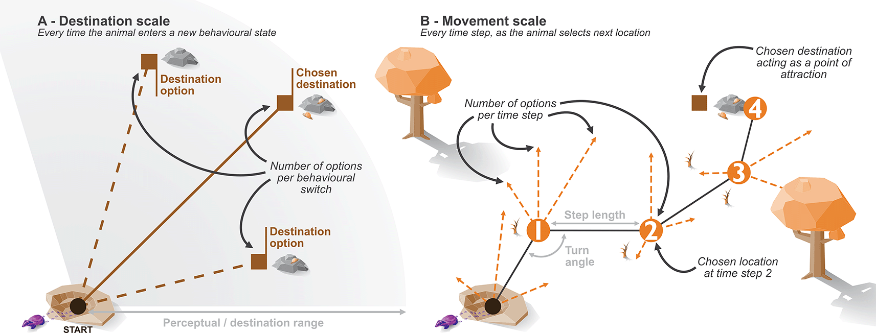
A - the time frame of the destination choice, B - the time frame of movements at each time step.
The animal has three behavioural states, broadly defined here as state 0 - sheltering (or resting), state 1 - exploring, and state 2 - foraging, that broadly define its movement characteristics and goals. In the sheltering state, the animal chooses a known shelter location to head towards; in the exploration state, the animal randomly moves within the landscape guided only by the movement resistance of the landscape; in the foraging state, the animal chooses a foraging location and moves towards it.
Additionally, each behavioural state modifies the movement characteristics of the animal; for example, exploring comprises of more random movements with longer distances between subsequent chosen locations, whereas sheltering behaviour is largely defined by stationary or very low discrete movements after returning to a shelter site. The movement characteristics are defined by two distributions: a Gamma distribution that step lengths are drawn from, and a Von-Mises distribution that turn angles are drawn from. The resulting step length, combined with a turn angle, describes the change in animal location between each time step (as selected from a given number of options). Here, we define these based on the movement capacity of the animal over a minute; however, there is no fixed underlying time frame for the simulation itself.
As the simulation will be running with three behavioural states, we need to define how likely an animal is to switch between the behaviours. We achieved this by creating a transition matrix that describes the probability at each time step of the animal changing to another behaviour [ Figure 2], where each value describes the probability of the animal transitioning from the current behaviour (row: b0 - sheltering, b1 - exploring, b2 - foraging), to the behaviour for the next time step (columns: b0, b1, b2). The diagonal describes the probability of the animal remaining in the same behavioural state. These probabilities can be kept high to introduce autocorrelation in the behavioural state; a high autocorrelation is required if we are modelling time steps as one minute. For the included example, we select probabilities that allow the animal to express all behavioural state reasonably evenly and allow behavioural cycles to be easily visible in the resulting simulated movement data.
##        b0      b1     b2
## b0 0.9700 0.01000 0.0010 # shelter
## b1 0.0002 0.95000 0.0008 # explore
## b2 0.0010 0.00001 0.9900 # forage
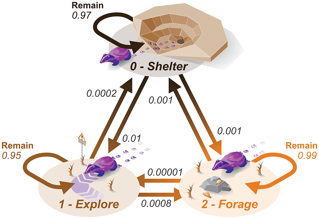
Remain values indicate the probabilities of the animal remaining in the same behavioural state. Values correspond directly to those in the transition matrix used as a simulation input.
Animals behaviour is frequently expressed via cycles, such as day/night or diel cycles61; therefore, we want the transition matrix to vary over time. We describe a number of cycles (or waves) that can be applied to the core transition matrix impacting the probability of entering sheltering behaviour. For example, a diel cycle can be expressed via a Sine wave with a frequency of 12 hours and an amplitude of 0.1. At each time step, we draw a value from the wave and add that weighting (from -0.05 to 0.05) to the transition probability of entering sheltering state (row 1, column 1 of the matrix); therefore, the probability of sheltering will increase and decrease following the Sine wave at a approximately 12 hour activity pattern. We can define as many cycles as needed, with varying frequencies, and they impact the sheltering probability additively.
When entering the sheltering behavioural state, the animal will seek out a shelter site. In the abmAnimalMovement package, we can supply a number of shelter sites to simulate this need and create site fidelity. As these shelter sites act as points of attraction for the animal, the animal occupies a consistent area, or something approximating a home range. Home ranges are meant to represent areas in which the animal can source all resources required for a given life stage.46 The predefined and steady state of these shelter sites provides the stability we look for in a home range, as well as a means of predefining a level of site fidelity. As the abmAnimalMovement model can have multiple attraction (rest) sites supplied, we can simulate home ranges with unequal and behaviourally influenced space use.
In addition to the predefined attraction to shelter sites, the abmAnimalMovement package allows for a more dynamic attraction to areas of high resource quality. Movements cannot be directly translated to animal preference; for example, habitat preference may miss key movement corridors,62 or the habitat decisions may occur at scales different to observed movement.1 Therefore, the simulation required a mechanism that somewhat detaches the preference/choice for observed movements. When entering the foraging behavioural state, the animal randomly selects foraging destinations as a point of attraction (weighted towards areas of higher quality) [Figure 1]. This desired destination remains constant for the duration the animal remains in the foraging state; subsequent times the animal enters the foraging state a new destination is selected. While in the foraging state, this destination attraction impacts the movement choices made at each time step, with the animal more likely to choose (and therefore move to) options closer to the foraging destination. Therefore, foraging destination choice operates on a different time frame to the movement and allows movements through low-quality foraging areas to reach a high-quality destination. This presents a critical benefit of the simulation approach, as we define the internal state decision making process of the animal. The two time frames also allow exploration of assumptions connecting simulated movement choices to choices grounded in resource use, and whether downstream analyses can accurately recover a hidden decision making process.
At all times, the subsequent locations of the animal are impacted by a movement resistance matrix. Differing values represent different environmental conditions that could change how easily/likely an animal is to use that area to move towards a destination. For example, rivers or hard barriers within a landscape could present very high movement resistance and an animal would aim to avoid traversing them. Alternatively, areas of lower movement resistance could aid movement, and potentially form movement corridors. The movement matrix has values that describe the weighting of movement probability (lower values indicating a lower probability of entering a cell). Whereas the resource environmental layer and shelter locations interact with destination/goal decisions, the movement resistance affects the step-by-step movement decisions.
The interplay between shelter sites, foraging quality, and movement resistance simulates the site fidelity required for home ranges, while allowing the environment to help shape the size and diffusion of that home range. Simulating a more dynamic and messy array of movements can help test how far assumptions of uniform circular animal movement are practical.
To demonstrate the variation that movement ecology methods need to wrangle, as well as the scope of movements the agent-based model can recreate, we provide three example species. The examples cover a range of movement capacities, site fidelity, and resting/sheltering patterns. Unlike alternative methods that are built to fit and simulate movements from existing data, our examples are loosely based on summary statistics from previous published results (cited below in each example species’ section). The choice of using species specific examples is intended to provide some biological context while demonstrating a range of simulation parametrisations. Therefore, we are only interested in whether the simulated data return the intended broad traits we are attempting to simulate for each example species (e.g., avoidance, site fidelity, expected step lengths). We show one example via a more detailed walk-through (badger), and the other example parametrisations are included as use cases at the end of the manuscript (vulture, king cobra).
2.3.1 Ecology and objectives - badger
Our primary example is based on a badger. Badgers occupy setts, in our example a two home/shelter sites, to where they routinely return.63,64 When not at the sett, the badger forages, and the foraging distances are impacted by resource position and movement capacity of the badger (i.e., how far can a badger feasibly travel for food from the sett). The badger therefore expresses very high site fidelity, a range dictated by the spatial positioning of resources, and is subject to the movement resistance of the terrestrial environment.
We can draw on studies such as Refs. 63 and 65 to roughly gauge the speed of badgers (i.e., step length per minute). How this speed differs between behaviours is more difficult to estimate from existing literature, but we can use Ref. 63 reported maximum speed to guide more direct movements (e.g., state 0 - sheltering and state 1 - exploring). In particular Ref. 63 mentioned the heightened speeds moving from and to the setts. We also want to allow the exploratory (state 1) movements to be great enough to occasionally exceed the normal home range or territory.66 We can draw on statements regarding maximum distance travelled in a night from papers such as, Refs. 63, 65 and 67 to approximate how distance foraging locations could be from a sett, While also confirming the nocturnal activity cycle for the badger. For the example, we will consider badgers as fully nocturnal, and with active periods lasting for around 8 hours each night.65,68 The 8 hour active periods are not consistent throughout the year. Badger occupying temperate areas are impacted by seasonal shifts that modify daylight hours and available resources.65,68 Badger movements are also impacted by their territoriality, avoiding areas occupied by other badger groups, but also displaying occasional extra-territorial movements.64,66 This suggests a general, but not complete avoidance of areas occupied by other badger groups.
We can broadly summarise the badger ecology we want to parametrise as follows:
The abmAnimalMovement package requires links to the Rcpp (>= 1.0.8.3)56–58 and BH (>= 1.78.0.0) packages,69 and therefore requires a version of R >=3.5.070 (available from www.r-project.org). Currently the abmAnimalMovement package can be installed from Github using install_github provided by the devtools package.69
While only the abmAnimalMovement package is required for running core simulations (abm_simulate function), to generate, organise, and review the inputs and outputs of simulations, we make use of a number of R packages. An alternative simpler implementation with no dependencies is provided as a package vignette.
library(abmAnimalMovement) # core package
library(dplyr) # data manipulation
library(reshape2) # data manipulation
library(ggplot2) # visualisation
library(ggforce) # visualisation
library(ggtext) # visualisation
library(ggridges) # visualisation
library(patchwork) # visualisation
library(raster) # environmental matrix generation
library(NLMR) # environmental matrix generation
We used R v.4.2.170 via RStudio v.2022.2.2.485,72 and used rmarkdown v.2.14,73–75 bookdown v.0.26,76,77 tinytex v.0.39,78,79 and knitr v.1.3980–82 packages to generate type-set outputs. We used the here v.1.0.1 package83 to help with relative file path definition. We used the dplyr v.1.0.9 and reshape2 v.1.4.4 packages for data manipulation.84,85 We used ggplot2 v.3.3.6 for creating figures,86,87 with the expansions: ggridges v.0.5.3,88 ggtext v.0.1.1,89 ggforce v.0.3.3,90 and patchwork v.1.1.1.91 We used the raster v.3.5.21,92 sp v.1.4.7,93–95 and NLMR v.1.196,97 for generating environmental matrices. NLMR is no long available on CRAN but still accessible here https://github.com/ropensci/NLMR, and installed using ‘remotes::install_github(“ropensci/NLMR”)’.
2.5.1 Generating environmental matrices
To ensure that the simulation completed during this example is repeatable, we set a seed. For the sake of simplicity, the year the examples were written (2022) is used.
seed ˂- 2022
set.seed(seed)
Before starting to simulate animal movement, we need to generate a landscape. The landscapes in this case will take the form of matrices, where each cell is describing the quality of foraging, shelter, and movement ease. The highest quality locations/cells are coded as 1, with quality decreasing as the values range down to 0. The 1 to 0 quality values in each cell are later used to help the animal to choose how and where it moves throughout the landscape. Depending on the behavioural state, the weighing of which matrix/layer to use will change (e.g., when in a sheltering behavioural state the shelter site quality layer is used).
For most applications, a landscape would be known a priori, but for this demonstration and testing of methods, we will use a selection of random generated landscape matrices [ Figure 3], using the NLMR package (neutral landscape models).
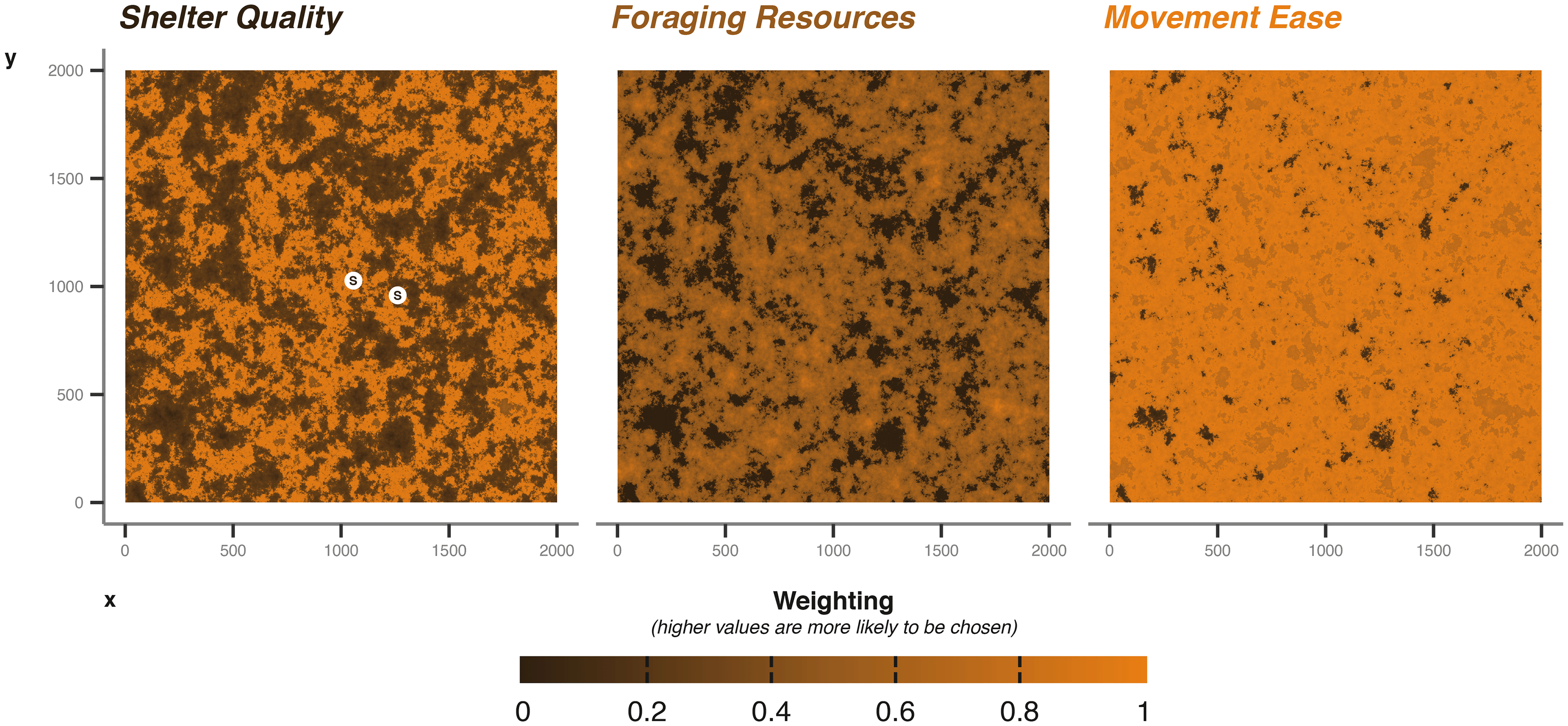
The points marked with S indicate the generated shelter sites randomly sampled from the underlying shelter quality matrix. X and Y axes cell numbers; in the case of the badger example cell is 5 m by 5 m.
We used a Gaussian field with an autocorrelation range of 40, a magnitude of variation across the landscape of 5, a magnitude of variation in the scale of autocorrelation range of 0.2, and a mean of 0.5. For foraging, we build on the Gaussian field already produced, allocating all values lower than 0.4 as 0 (i.e., no value for foraging), then normalising the remaining values between 0 and 1.
For a baseline movement resistance layer, we take the original Gaussian field and increase areas greater than 0.6 by 0.5 to allow areas of high resource quality to be easily accessible. We also greatly increase the movement ease in “edge” habitat (+1), where values fall between 0.6 and 0.3. Again we normalise between 0 and 1, where 1 are areas easily traversed. The resulting environment is one with easily traversable edge areas, surrounding better quality foraging locations than can be moved into easily.
Shelter quality is intermediate; we increased weighting by +1 in areas where cell values were greater than 0.5 and lower than 0.7. Thereby shelter sites are more likely to occur in the areas of higher foraging quality, but not in the core (i.e., >0.7), nor in the edge areas (<0.5). This provides some balance between accessibility and proximity to resources. The three matrices described provide a baseline for our examples, but can easily be modified for different scenarios [ Figure 3]. To aid balancing, we keep values between 0 and 1; any numeric value can be used, but the simulation will interpret the values as relative weights when the animal is making decisions (Note: The current implementation of cpp_get_values that extracts values from the matrices during the simulation returns -99.9 weighting when presented with NA values; therefore, -99.9 serves as a lower limit to the matrix weighting values).
Once generated will supply the core simulation function (abm_simulate) with each of these layers via the shelteringMatrix, foragingMatrix, and movementMatrix arguments (Table 1).
Arguments are the terms used in the function, the inputs are the R objects created during this example, the descriptions provide a brief overview of what the argument is configuring.
2.5.2 Animal parameters
We predefine a suite of parameters describing the movement and behaviour characteristics of the animal (e.g., badger) loosely based on summary statistics and general statements from previous research (e.g., Refs. 63–68). We store the parameters as objects we can later input into the abm_simulate function. We complete this process for three species; the badger values are displayed below, whereas the values for vulture and king cobra examples are provided at the end of the manuscript.
We parametrise shelter information in the following ways. For the sett, we draw two sets of coordinates from the shelter quality layer. During the simulation, the badger will randomly select a sett to return to each time it enters the sheltering behavioural state. The choice of which sett to return to is weighted by the values supplied via the shelter quality environmental layer [ Figure 3]. The coordinate data frame is provided to the core simulation function’s shelterLocations argument.
The shelterSize argument describes the radius around the shelter locations within which the animal exhibits near stationary behaviour. We specify the shelter size to be 8 m, meaning that when within 8 m of the selected shelter site the animal’s possible step lengths are decreased 100-fold. The shelter site size of 8 m allows for small movements near/within the sett during sheltering behaviour.
sampledShelters ˂- sampleRandom(raster(landscapeLayersList$shelter), 2,
                                ext = extent(0.45, 0.65, 0.45, 0.65),
                                rowcol = TRUE)

BADGER_shelterLocs ˂- data.frame(
 "x" = sampledShelters[,2],
 "y" = sampledShelters[,1])

BADGER_shelterSize ˂- 8
Badger movement is set via the definition of three pairs of Gamma and Von Misses distributions. Each behavioural state is provided with a Gamma distribution to describe the step lengths between locations, and a Von Mises to describe the turn angles. When combined these two distributions provide the animal with a number of locations to choose from at each time step [ Figure 1]. As we have three behavioural states, each movement parameter takes the form of a vector of length three. The step lengths require predefined shape (k) and scale (θ) parameters to describe the Gamma distributions, and we provide these to the simulate function via the k_step and s_step arguments. For the turn angles, we require the mean (μ) and concentration (κ) to defined the Von Mises distributions and provide these via the mu_angle and k_angle arguments.
The perceptual range (implemented here as destination range) is how far the badger can “see” when deciding where to forage and is set in a similar fashion. Where destinationRange provides the shape (k) and scale (θ) for the Gamma distribution describing distance of possible foraging locations, and destinationDirection provides the mean (μ) and concentration (κ), the Von Mises distribution describes the angle at which those locations can fall in relation to the previous direction of movement [ Figure 4].
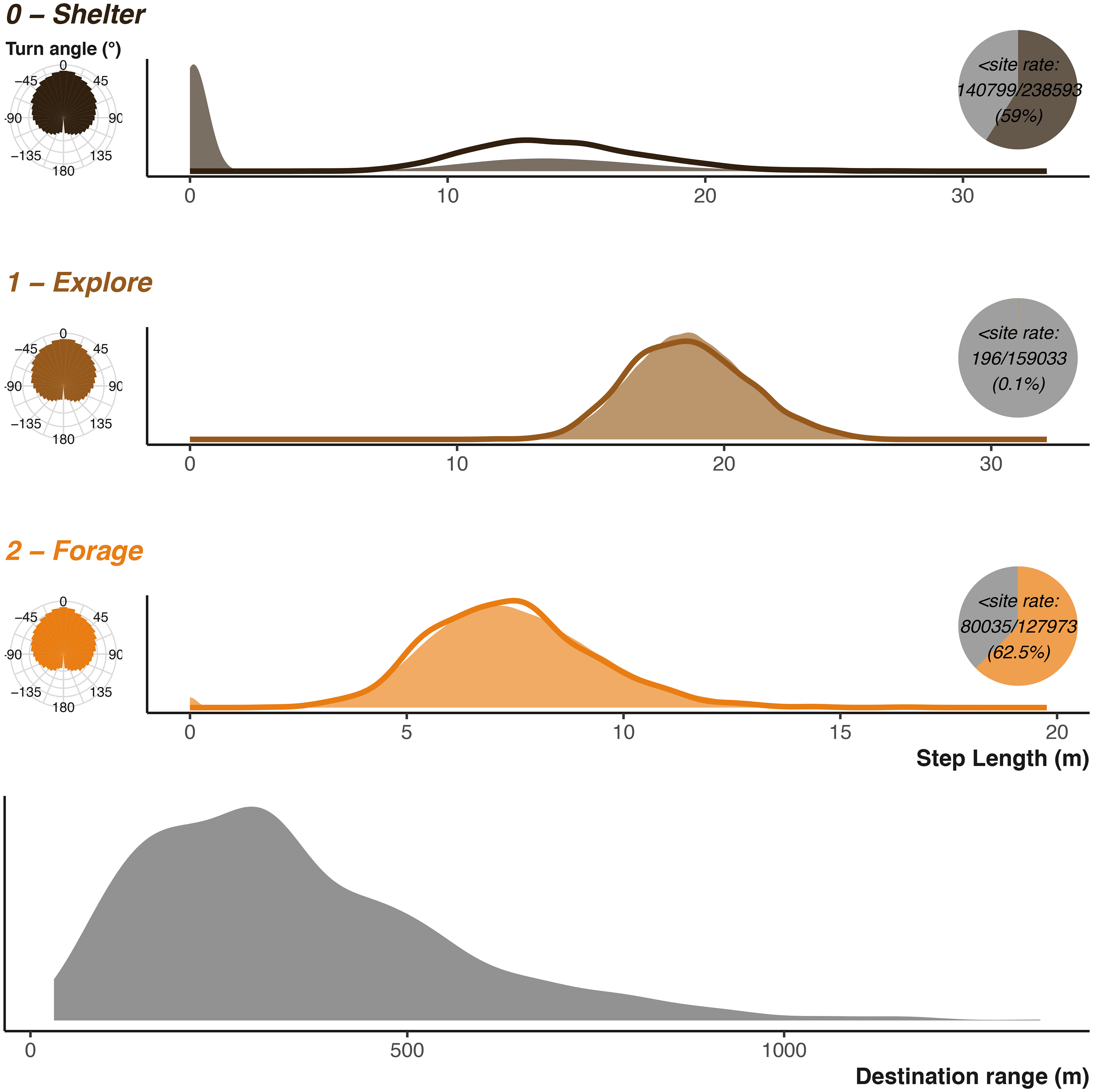
Parametrising distributions are shown as solid areas using the same shape and scale parameters used as input into the simulation function. The lower plot shows the distribution used to generate potential foraging destinations. The realised resulting simulated step lengths (scaled to the input units) are shown by the solid lines. The realised resulting turn angles are shown in left hand sub-plots. Inset pie charts show the number of step lengths that were below the shelter site size. Note that x axis is not consistent between the three plots.
We can also alter the strength of attraction to the foraging destinations. At each time step, the animal is offered a number of location options to move to next time step. The simulation calculates the distance between all options and the destination (i.e., a foraging location or shelter site), then normalises the distances between 0 and 1. The normalises values serve as weighting to increase the chances the animal will move towards its destination. We modify the weighting with the destinationTransformation and destinationModifier arguments. The destinationTransformation allows for weightings to be transformed (where 0 = no transformation, 1 = weights are square-rooted, 2 = weights are squared). Values supplied destinationModifier applies a linear multiplicative effect to all the weightings. When these weightings increase in value, the animal will exhibit a stronger attraction and choose more direct movements to its current destination.
We also store a value ready for the rescale_step2cell argument. The rescale value is a simple means of adjusting the environment layers to fit with the scale/unit in which the step lengths are provided. In this case, we treat each cell as 5m by 5m, thereby ensuring that our 2000x2000 matrix is sufficient for the badger to traverse without leaving the extent of the generated landscape. The rescale value therefore allows high resolution movements on lower resolution environments, offering a crucial memory saving optimisation.
BADGER_k_step ˂- c(0.3*60, 1.25*60, 0.25*60)
BADGER_s\_step ˂- c(0.8, 0.25, 0.5)
BADGER_mu_angle ˂- c(0, 0, 0)
BADGER_k_angle ˂- c(0.6, 0.99, 0.6)

BADGER_destinationRange ˂- c(3, 120)
BADGER_destinationDirection ˂- c(0, 0.01)
BADGER_destinationTransformation ˂- 2
BADGER_destinationModifier ˂- 2

BADGER_rescale ˂- 5
The territoriality is not simulated directly via other individuals. Instead we approximate it by supplying a number of point locations the badger will avoid. An alternative way of simulating this behaviour would be to create areas of high movement resistance to prevent the badger from entering. We provide a set of x, y coordinates of locations to be avoided. Alongside the locations, we need to define how strongly the badger will avoid them using avoidTransformation (distance to point is weighting squared) and avoidModifier (distance to point is weighting multiplied by 4). Both avoidTransformation and avoidModifier operate in the same way as the destination attraction arguments, but inverted; therefore, the avoidance behaviour will directly counteract the attraction to destination behaviour.
BADGER_avoidLocs ˂- data.frame(
 "x" = c(1205, 1500, 1165),
 "y" = c(980, 1090, 1250))

BADGER_avoidTransformation ˂- 2
BADGER_avoidModifier ˂- 4
We implement two cycles to capture the daily and seasonal cycles the badger experiences. Both cycles are created by describing a Sine wave defined by its amplitude, midline, offset (ϕ) and frequency (τ; via the cycle_draw function). The abm_simulate function has two arguments for wave parameters: rest_Cycle is a mandatory input to describe diel activity cycling, and additional_Cycles to define any number of additive additional cycles. For rest_Cycle, we will store a vector of length 4, with values defining the amplitude, midline, offset, and frequency in that order (Frequency is supplied in hours, i.e., 60 times the time step). We set the amplitude to 0.12 and midline as 0, meaning the probability of sheltering will be modified by values ranging from -0.06 to 0.06 depending on the location in the wave. Our badger example requires a 24 hour cycle where the probability of sheltering will peak and nadir, hence offset and frequency are set to 24 hours. When combined with the base transition probability to shelter, the above parametrisation creates a scenario of approximately 8 hour periods of activity every 24 hours.
To add a seasonal cycle, we will use additional_Cycles. We predefine a data frame where each row contains four elements describing the amplitude, midline, offset, and frequency. Whereas our diel activity is defined by a 24 hour cycle, a seasonal cycle is 365 days, and we shift the peak half a year (offset = 365/2). The seasonal wave will increase the probability of sheltering behaviour during a portion of the year, while not also overwhelming a relatively stable diel cycle (i.e., badger will sleep longer during one part of the year) as we have set a lower amplitude for the seasonal cycle (0.075). A more extreme implementation of the second cycle could introduce hibernation behaviour.
We also pull forward the behaviour transition matrix we showed during the overview, and rename it so all simulation input objects have the BADGER_ prefix.
BADGER_rest_Cycle ˂- c(0.12, 0, 24, 24)

# additional cycle
c0 ˂- c(0.075, 0, 24* (365/2), 24* 365) # seasonal

BADGER_additional_Cycles ˂- rbind(c0)
BADGER_additional_Cycles

##     [,1] [,2] [,3] [,4]
## c0 0.075   0 4380 8760

BADGER_behaveMatrix ˂- Default_behaveMatrix
BADGER_behaveMatrix

##        b0      b1     b2
## b0 0.9700 0.01000 0.0010
## b1 0.0002 0.95000 0.0008
## b2 0.0010 0.00001 0.9900
2.5.3 Running the simulation
We need to initially define a start location for our animal. To introduce some more individual variation, we can randomly vary this starting location, but we will restrict the start locations to be proximal to the centre of the environment. For the simulation, we need a vector of length 2, where the first value is the x location, the second is y.
startLocation ˂- sample(900:1100, 2, replace = TRUE)
We finally have some parameters that describe the scope and intensity of the simulation. The length of the simulation is provided via the timesteps argument; in our examples, we are operating under the assumption that one time step is equal to one minute. Equally timesteps can be thought as the number of movement choices simulated. We also need to specify how many options will be drawn and considered by the animal at each time step. The options argument is where this is input. Similarly, des_options is where we specify the number of dynamically selected foraging attraction/destinations to choose from when it enters the foraging behaviour mode (state 1).
We can then call all our settings describing badger behaviour and movement settings we stored as objects previously, and run the simulation using abm_simulate (Table 1).
The simulation function (abm_simulate) outputs a list containing: (1) a dataframe of realised simulated movements, (2) a dataframe of options the animal had available, and (3) a list of the inputs used to simulate the movement. The realised movement dataframe (locations) describes all simulated locations the animal occupied, step length information, behavioural state, and current point of attraction, where each row is equal to a time step. Note the simulation is scale agnostic, so each row can represent a different time step to the example. Other than the lack of timestamps and location error, the format largely mirrors a typical movement dataset. Our example is minute by minute; changing what the time step represents would require a reparametrisation of step length and behavioural transition probabilities. The options dataframe describes all the options available to the animal over the entire simulation duration, where each row is equal to an option repeated for each time step.
Once simulated, we can review the movement characteristics of the three species. The simplest to examine is the movement speeds or step lengths. During the simulation parametrisation we provided rescale values for the size of the cells describing environmental information (see rescale_step2cell argument). The simulated movement will return the scaled values, so to plot something comparable to the input values, we must rescale the simulated step lengths.
We can compare the simulation’s inputs displayed in Figure 4 and see that they largely agree as expected. The discrepancy in the sheltering behaviour is due to the elevated instances of negligible movement once the animal has reached their chosen shelter site. The turn angles are more variable, as the destination decisions and attraction to locations heavily influence the distribution overriding the initial parametrisation of the Von Mises distribution. Figure 11 and Figure 12 in the uses cases section show the outputs for vulture and king cobra simulations.
We can review how the movements appear in space. With the badger example, the impact of the avoidance points is clearly visible [ Figure 5A], whereas the lack of or weaker avoidance in vulture [ Figure 5B] and king cobra [ Figure 5C] makes the avoidance less influential. The vulture’s movements and chosen foraging locations are largely to the east, demonstrating the impact of the underlying foraging quality environmental layer. The king cobra plot shows the impact of a near impermeable barrier truncating the southward movements.
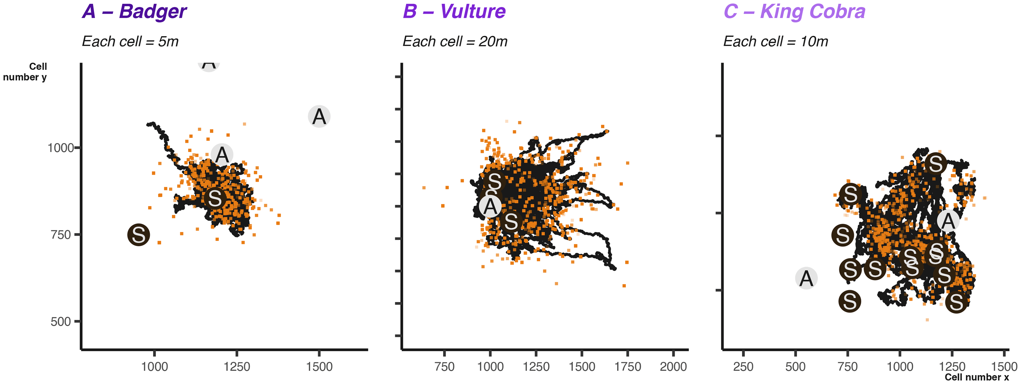
Black points show the simulated location at each time step. The orange squares show the dynamically selected foraging destinations. Circles with an interior S show the shelter site locations, and circles with an interior A show the avoidance points. Note that the size represented by each unit on the x and y axis differs depending on the species as governed by the rescale argument.
The activity cycles and the timing of behavioural shifts is a key component in the simulations. We can examine that the predefined cycles result in expected patterns. A year of data makes observing all but the broadest cycles difficult, so in Figure 7 we can look at several months of data as well as the daily cycle. Badger and vulture daily cycles are largely the same [ Figure 7A & B], with a consistent daily activity cycle differing only slightly in the time spent active and balance between shifts from sheltering to foraging and exploring. Some of the differences are a result of the different behavioural transition matrices provided to simulate the two species, where both had different baseline probabilities of shifting between behavioural states. By contrast, the king cobra example demonstrates the interaction between the daily and weekly cycles [ Figure 8]. We can see intermittently extended sheltering periods, punctuated by short exploratory or foraging bouts.
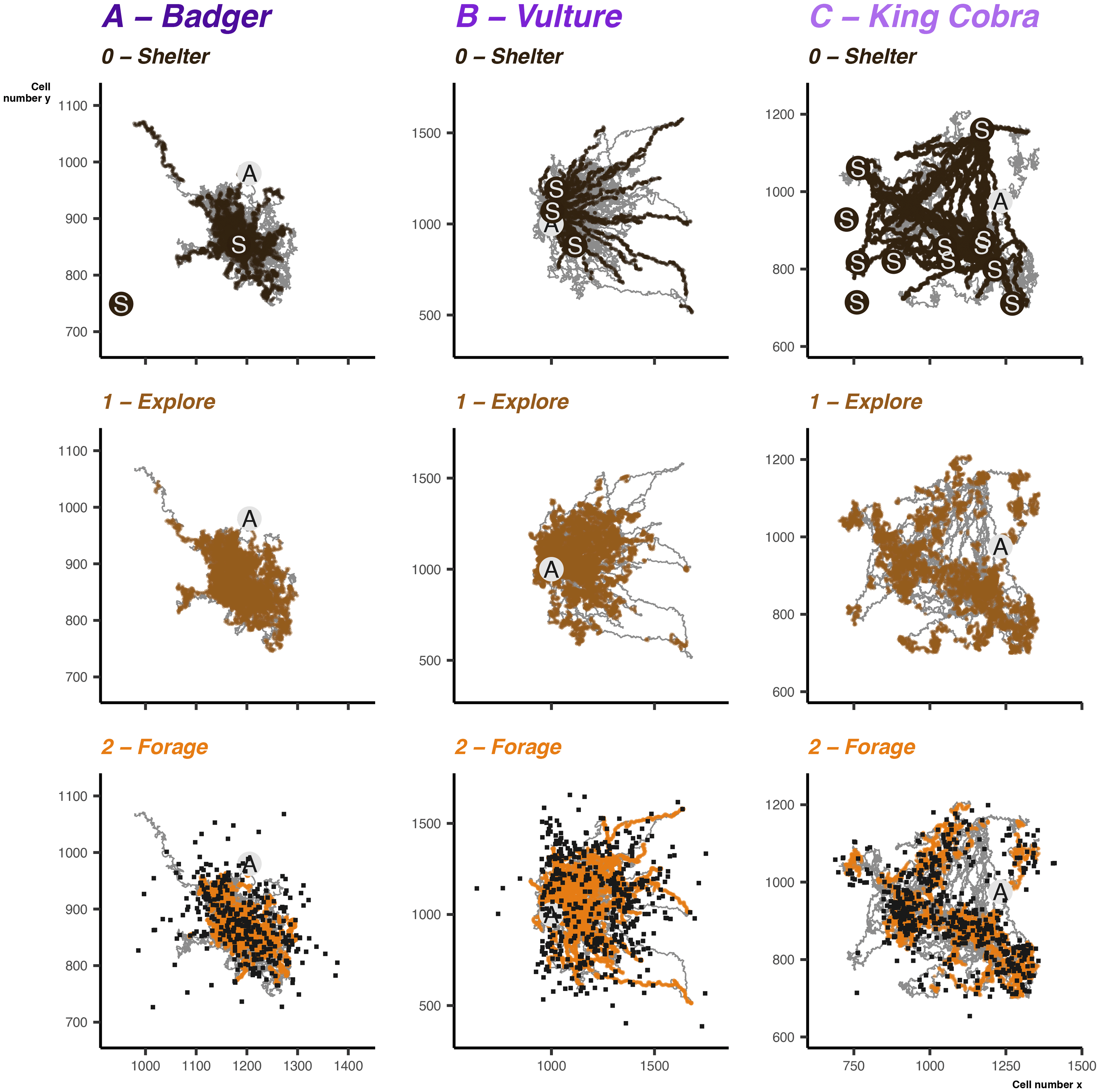
Grey path shows the overall movement during that month, overlaid points indicate where the animal was in a given behavioural mode. Circles with an interior S show the shelter site locations, and cricles with an interior A show the avoidance points, black squares show the dynamically selected foraging destinations. Note that the size represented by each unit on the x and y axis differs depending on the species.
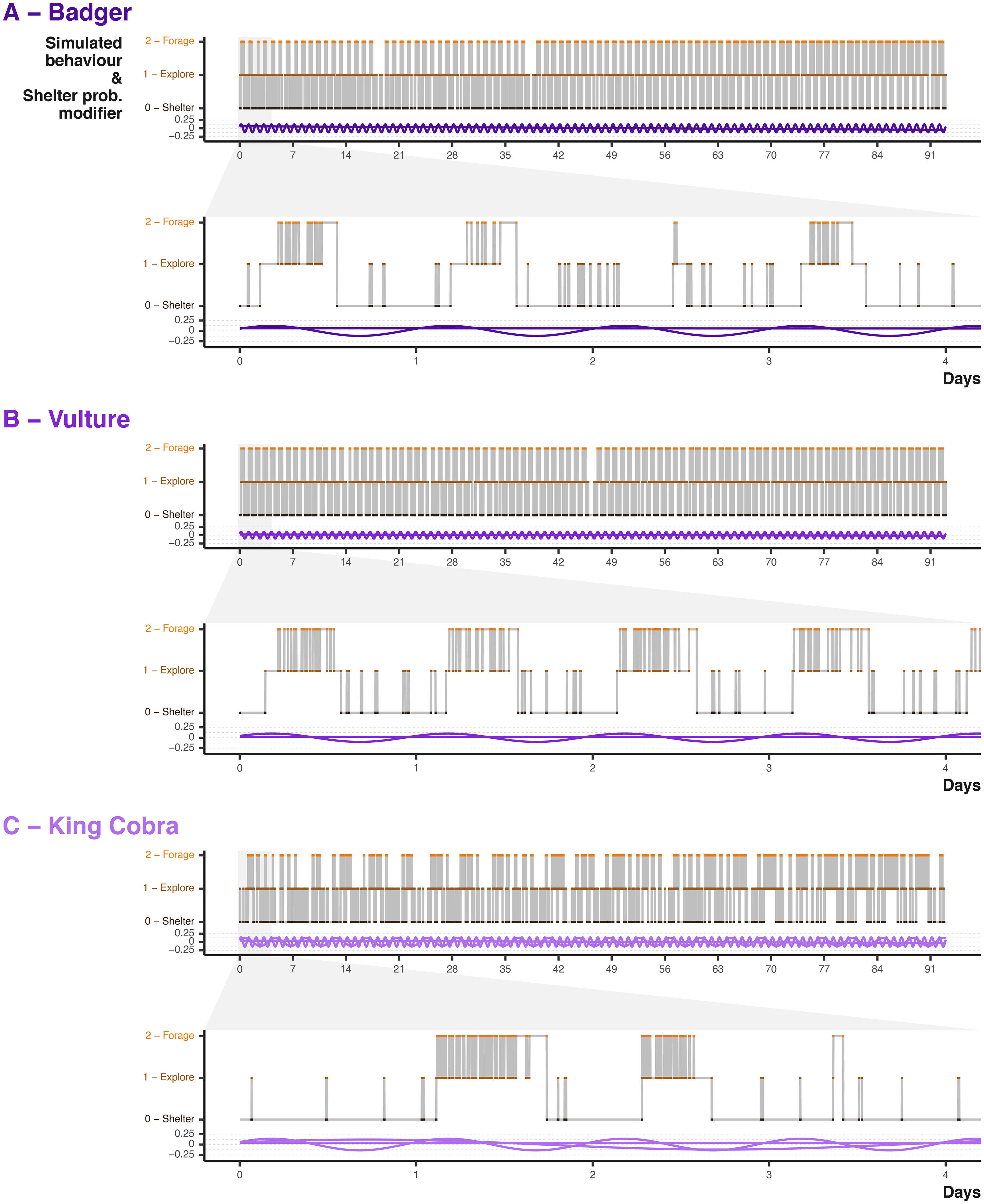
Point colour and position describe the behavioural state at each simulated time step, whereas the purple waves indicated the input values. That the input shelter probability waves are additively combined with the underlying behavioural transition matrix of each species.
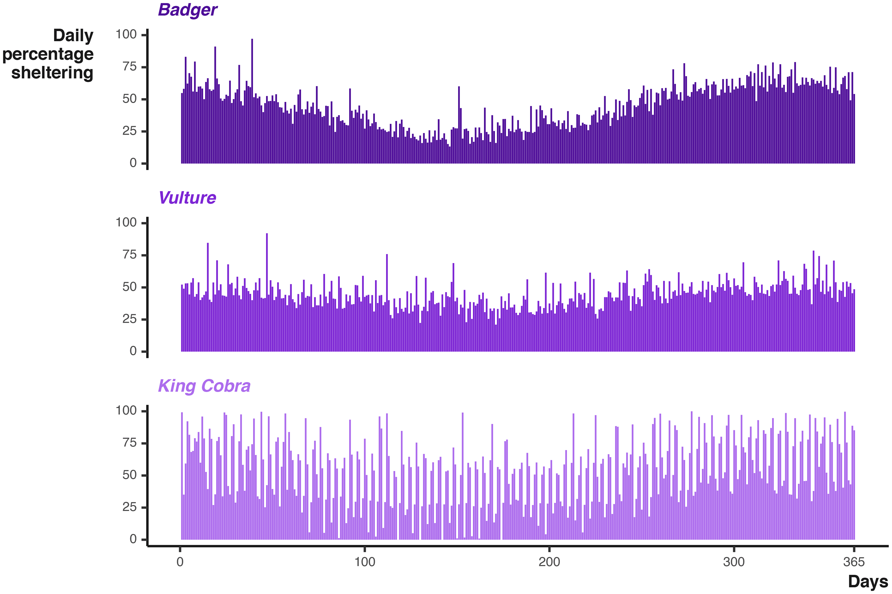
At the daily and monthly scale, we cannot see the impact of the broad scale seasonal cycles. Instead we can look at the percentage of time steps per day the animal was in sheltering behaviour [ Figure 9]. Again the Badger and Vulture sheltering rates are similar, differing in intensity, but with both demonstrating a seasonal decrease in the middle of the simulation. The king cobra cycles reveal decrease in the number of days spent entirely sheltering and an overall impression that the seasonal cycle is less influential (as it is only one of three activity cycles).
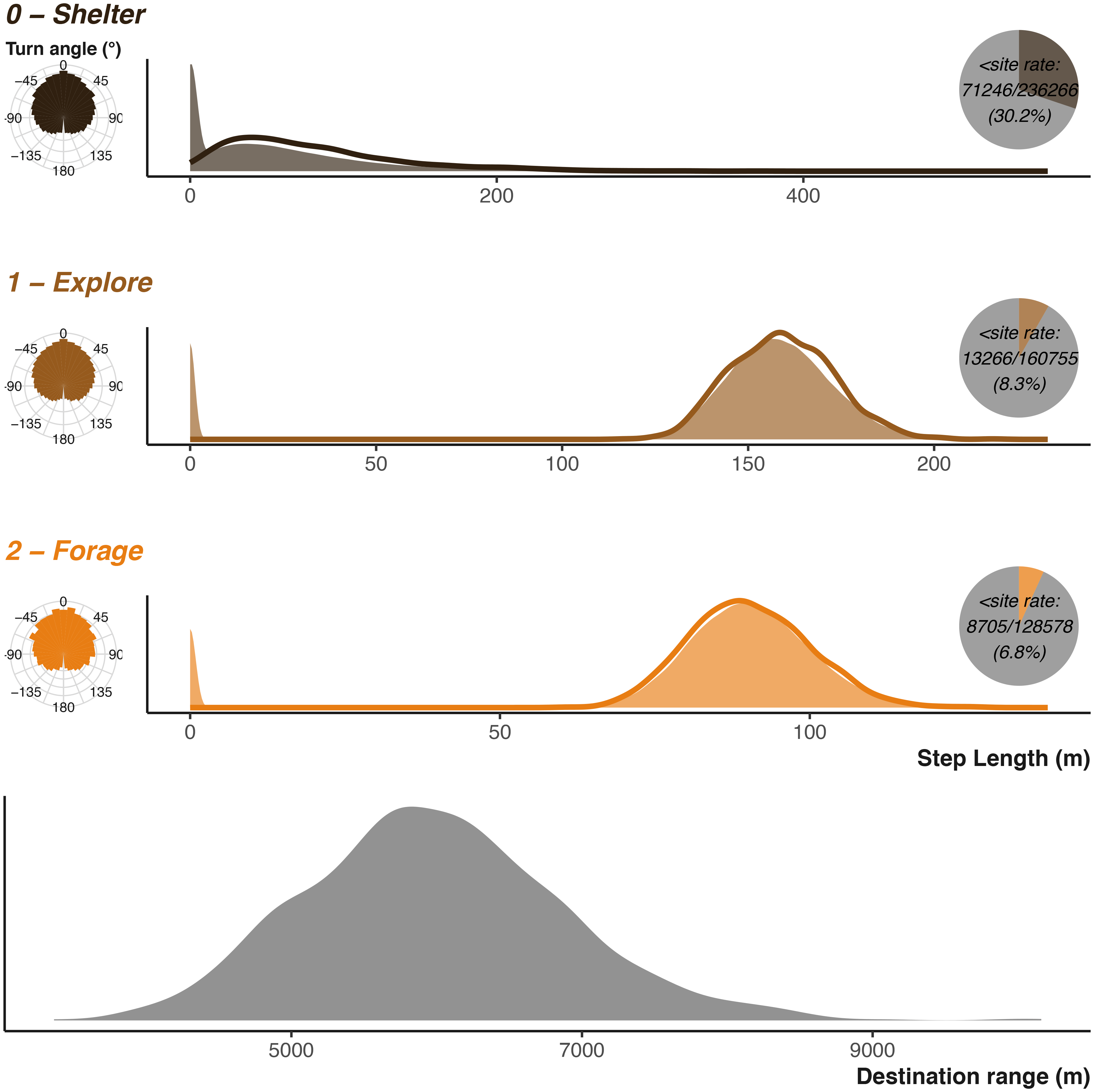
Parametrising distributions are shown as solid areas using the same shape and scale parameters used as input into the simulation function. The lower plot shows the distribution used to generate potential foraging destinations. The realised resulting simulated step lengths (scaled to the input units) are shown by the solid lines. The realised resulting turn angles are shown in left hand sub-plots. Inset pie charts show the number of step lengths that were below the shelter site size. Note that x axis is not consistent between the three plots.
Animal movement datasets are complex and require a suite of analytical approaches to tackle satisfactorily. Efforts to develop new, and test existing, analyses would be aided by access to a range of diverse datasets. While ideal simulations often accompany new analysis methods and provide superb validation for the method in question, reaffirming the method’s robustness and pushing them to new limits with a messier, more stochastic, simulation approach could greatly strengthen our confidence in results. The abmAnimalMovement package provides an independent route to test new methods, which covers a range of interacting movement features, not necessarily directly tied to a single analytical method. For example, we have used this simulation to explore the impacts of analysis choice on researcher’s ability to extract habitat selection estimates from movement data.54,55 By knowing the underlying mechanism of habitat selection, we are able to state whether analysis methods returned corrected or expected results, while quantifying how different analytical choices led to uncertainty.
By including a range of features linked to movement and behaviour, the abmAnimalMovement package can be implemented to investigate a suite of questions commonly asked of movement data –from habitat selection, to behaviour detection (for examples of common themes see Ref. 13). While some of the features can appear simplistic, there remains ample flexibility to simulate a wide range of useful scenarios. For example, we conceptualise the three movement states as sheltering, exploring, and foraging. However, only several aspects are immutable: one state exhibits site fidelity (state 0), one state is free from all attraction (state 1), and one state is driven by an underlying environmental layer (state 2). Reduction to a two or one state scenario could be achieved via manipulation of the transition probabilities. For animals demonstrating more behavioural states, the abmAnimalMovement package would need considerable extension to be useful; the same for migratory species, especially those travelling long distances into mutually exclusive areas.
The abmAnimalMovement package has an advantage over data-driven simulation methods in scenarios where data are scarce, as much of the animal world is untracked.13,25 For the untracked animals, we may be limited to basic information of speed, activity, and resources, or such information may even need to be inferred from ecologically similar species. In such data starved situations, the abmAnimalMovement package’s low computational cost and minimal data requirements allows for a large number of alternative parametrisations to be explored. Via the explorations of different parametrisations, researchers can help build a picture of the study and analysis methods best suited for their questions, with the opportunity to test those analyses on synthetic simulated data.
In cases where data cannot be shared (e.g. due to concerns over species sensitivity), using a synthetic dataset could allow researchers to provide peer reviewers a dataset to test and error-check analysis code.98 Providing data is a key component to ensuring computational reproducibility,99 and synthetic datasets provide an avenue to limit the reproducibility loss from data sharing restrictions. Additionally, such synthetic datasets could be integrated into preregistration as a means of demonstrating the validity of an analysis plan prior to undertaking a study, or as post hoc exploration of sampling uncertainty.35
Producing a range of simulated datasets that cover alternate scenarios may present researchers with opportunities to test real data against a null model. For example, researchers looking to investigate whether an animal was avoiding a certain landscape feature could calibrate a number of simulations covering a range of differing avoidance strengths. The simulated results could then be compared to the real data to gauge how different the real data was from simulations exhibiting zero avoidance (i.e., a null model scenario). This approach could complement current analysis methods, akin to sensitivity analysis.
The abmAnimalMovement package provides adequate functionality to simulate a range of scenarios and movements. However, there are several aspects that will bear updating in future versions.
1. Dynamic state 0. While state 0 and the steady state of the attraction locations is key to simulating range stability (i.e., home range), there maybe scenarios where this stability is not desired. For example, simulating dispersal behaviour of juvenile or sub-adult animals there may be a desire to have shelter site dynamically chosen for a time. Currently such behaviour could be simulated, but it would require the dispersal to occur immediately, and the dispersal destination to be predefined (i.e., the sites for state 0 attraction). Therefore, in the current state the package may be limited in its ability to help predict possible dispersal destination, but potentially capable of informing dispersal routes.
2. Autocorrelated speed. We may need to improve the autocorrelation of the animal’s speed. Currently the speeds are non-independent based on the behavioural mode of the animal. The need to implement a more aggressive movement momentum/autocorrelative structure may be felt more acutely at different time frames, and for animals with a great variation in step lengths (i.e., a larger θ for the Gamma distribution). Explorations of simulated data using methods that measure autocorrelation in animal speed will reveal how much of a priority this should be.
3. Dynamic environment. All the environmental matrices are static; currently there is no system to update values during the simulation. This prevents shifts in the landscape such as seasonal variation in resources, or the development of trails. Currently, the closest solution is to run multiple simulations where the end location of simulation1 is the start location for simulation2, where simulation2 is provided with a new season-appropriate resource layer. This solution would be inadequate for trail development, as trail development would require a system within the simulation to update previously used cells for the animal at each time step.
This section provides alternative parametrisations for the secondary examples to better demonstrate the range of movement types and scenarios the abmAnimalMovement package can replicate. Primarily, we created these further examples for use in Ref. 54, 55, to broaden the generalisablity of the findings explored in those papers. We provide example implementations of vulture and king cobra-like movement.
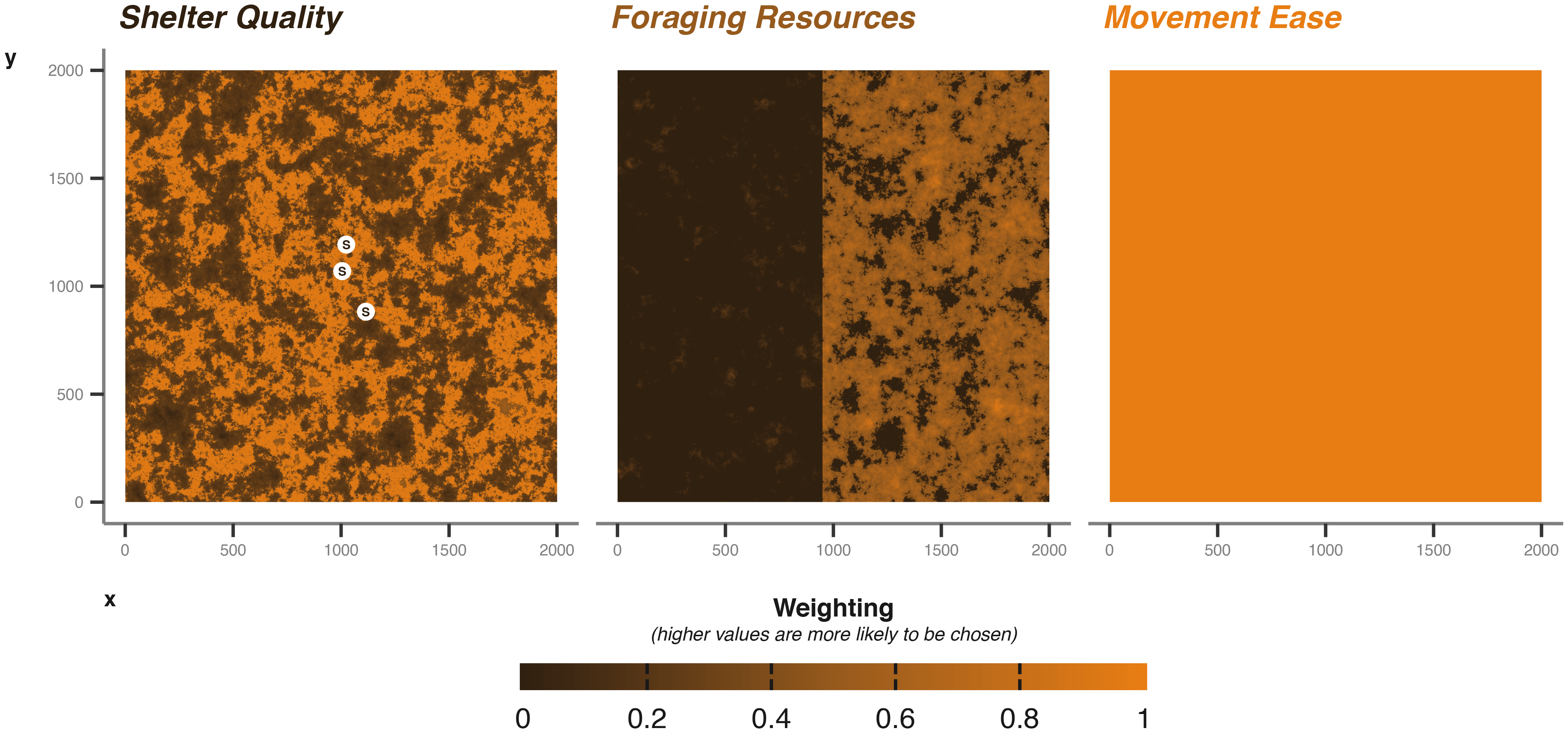
Unlike badgers and other terrestrially moving animals, vultures can move great distances with minimal obstruction [ Figure 9]. Vultures can also move greater distances more rapidly,100 resulting in a more variable and distribution of step lengths101–103 [ Figure 9].
Similar to badgers vultures exhibit significant site fidelity, re-using roosting and nesting sites.104 Such shelter sites could be predefined; for example, if shelter sites were known a priori discovered via the capture and tagging of animals, which in the case of birds is more likely.
Vultures also offer an opportunity to demonstrate how the underlying resource availability impact the movements of animals. Their moments have been seen to follow carcass, creating starkly contrasting areas where vultures will and will not travel9 [ Figure 10].
Vultures have a very similar cycle pattern to the badgers (just inverted), one defined by a standard 12 hours of activity during the day, and 12 hours of increased sheltering behaviour during the night. The importance of simulating such cycles is made clear by vultures studies demonstrating that day-night cycles can impact rates of location collection.105 How the animals’ activity cycle and the probability of collected data interact could be key consideration for some research questions. Again similar to badgers we would expect seasonal shifts in the form of an increase and decrease in activity depending on the time of year.100–102,106
We can broadly summarise the vulture ecology we want to parametrise as follows:
4.2.2 Ecology and objectives - king cobra
Whereas the previous two species have a very limited or single shelter sites, king cobras make use of a wider range of shelter sites distributed more widely over their home ranges.107,108 These sites can also be larger, comprising burrow systems or rock complexes.
What more dramatically sets king cobras, and other snakes, apart is a vastly differing shelter-forage cycle. While snakes still exhibit a diel cycle, the intermittent depredation of large prey items and the time required sheltering to digest large meals results in a second broader activity cycle operating over a more widely observed diel cycle.108–111 We can conceptualise this pattern as two additive cycles, one that will describe the daily activity cycle, and a second that describes the foraging and digestion cycle. Seasonality also impacts king cobra activity. As king cobras occupy tropical regions, the seasonality they experience is not as pronounced as the badger or vulture examples. Overall king cobras have three activity cycles acting on three different scales.
In this example, we can also demonstrate the movement resistance dramatically impacting movement possibilities. King cobra movement can be limited by roads,112,113 where unless provided with crossing structures king cobras are vulnerable to vehicle hits [ Figure 11]. In addition to roads presenting linear barriers across the landscape, king cobras face persecution when near or in human settlements.113,114 Despite the risks, avoidance of such areas appears weak.
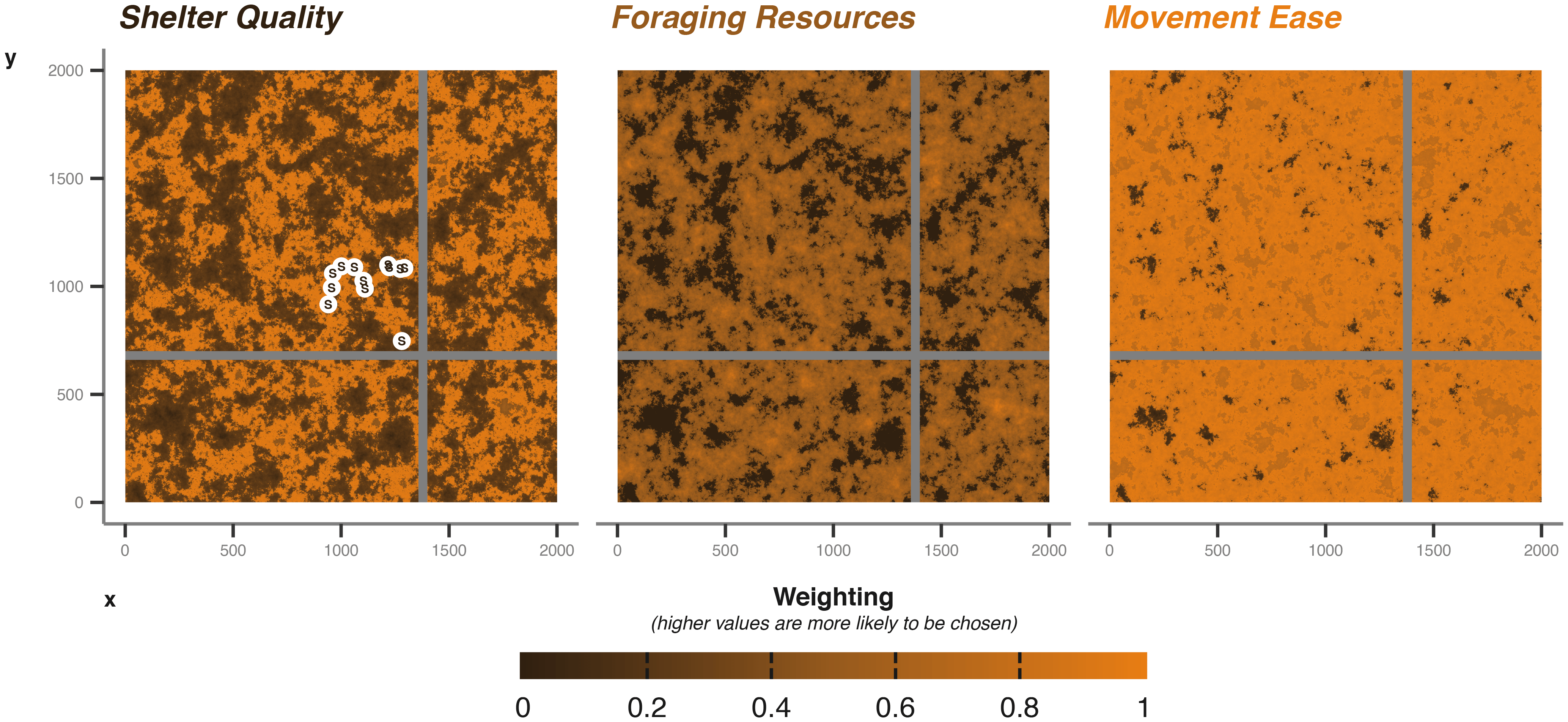
Movement ease is blocked by bars of -99 weighting.
Finally, king cobra movement characteristics will be dramatically reduced compared to the vulture’s, but with similar shape to the badger with greater variability [ Figure 12] as king cobras are known to range over large areas.107,108,115
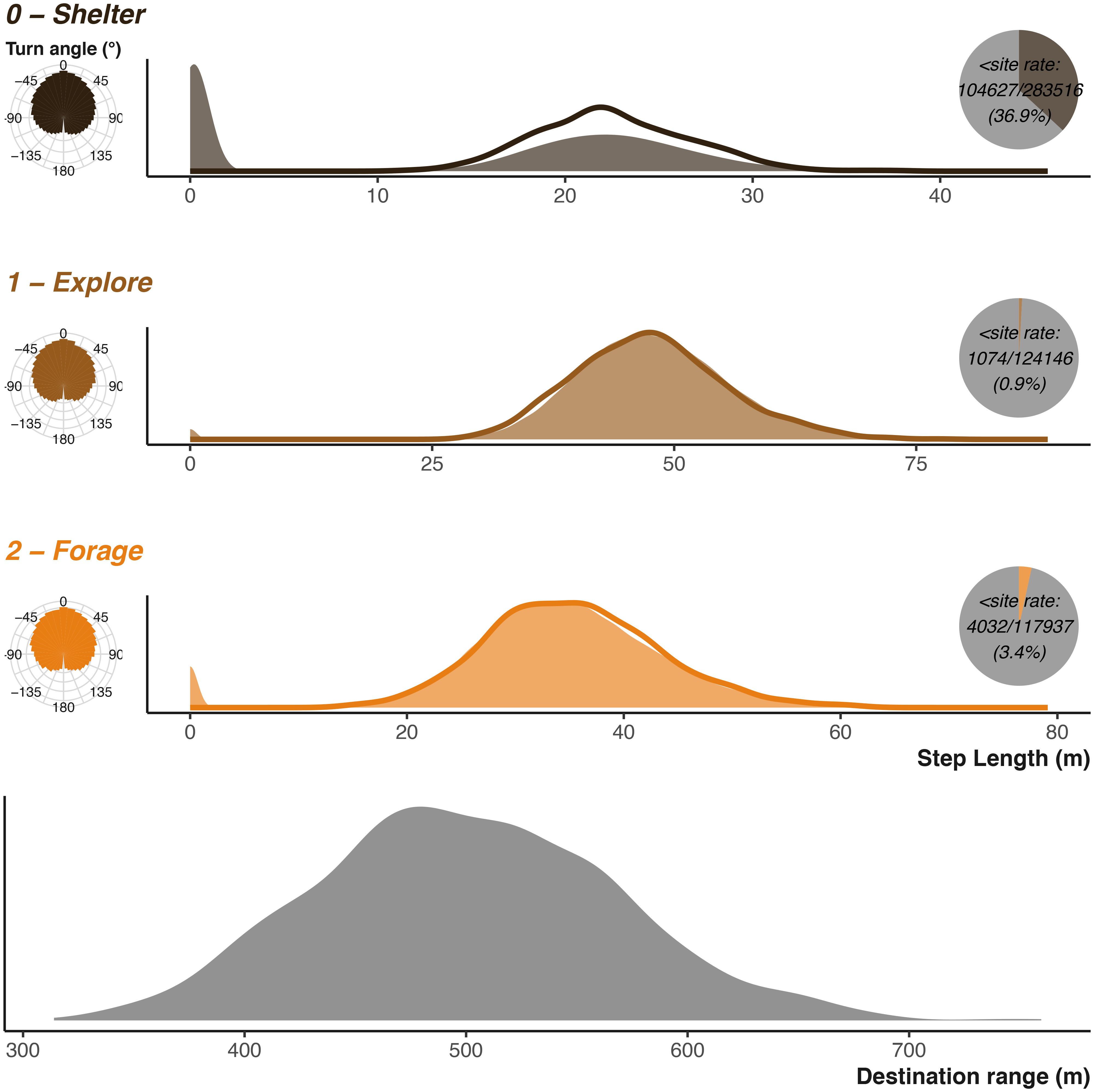
Parametrising distributions are shown as solid areas using the same shape and scale parameters used as input into the simulation function. The lower plot shows the distribution used to generate potential foraging destinations. The realised resulting simulated step lengths (scaled to the input units) are shown by the solid lines. The realised resulting turn angles are shown in left hand sub-plots. Inset pie charts show the number of step lengths that were below the shelter site size. Note that x axis is not consistent between the three plots.
We can broadly summarise the king cobra ecology we want to parametrise as follows:
1. Lower site fidelity via the use of many shelter sites107,108
2. Movement speed approximated by summary statistics from previous studies,107,108,115 with examples of very high landscape derived resistance112,113
3. A 8-12 hour activity cycle, with approximately weekly forage-digest cycle, and weak seasonality108–111
4.2.3 Simulation inputs
Vulture Inputs The vulture parametrisation largely the vulture parametrisation matches the badger. We specified a number of predefined resting/shelter sites, assuming that bird bio-tagging is more likely to occur at known site (i.e., nests or roosts). The shelter site size is smaller than the badger sett, so is only 5 m. Step length parameters are all larger and more variable, along with destination ranges [ Figure 11]. We also set a larger rescale value to ensure the vulture has a larger landscape to operate across. The shelter cycle is broadly similar, with a 12 hour diel cycle and gentle seasonality. We make two small modifications to the transition matrix allows for more frequent switches between foraging and exploring. We also alter two of the environmental matrices. We maximise movement ease across the entire landscape, while also lowering the foraging quality for an area to the West reflecting lower resources in that area [ Figure 9]. Finally, we specify that the vulture will not be avoiding any locations; we still require inputs for the simulation, but we can provide zeroes to negate the effect.
# predefined shelter sites
VULTURE_shelterLocs ˂- data.frame(
 "x" = c(1024}, 1005, 1115),
 "y" = c(1193, 1070, 882))
# shelter site radius to reduce movements
VULTURE_shelterSize ˂- 5

# parameters defining Gamma (step length) and Von Mises (turn angle) for each
# behaviour state
# Gamma shape
VULTURE_k_step ˂- c(2, 2.2*60, 1.5*60)
# Gamma scale
VULTURE_s_step ˂- c(40, 1.2, 1)
# Von Mises mean
VULTURE_mu_angle ˂- c(0, 0, 0)
# Von Mises concentration
VULTURE_k_angle ˂- c(0.6, 0.99, 0.6)

# parameters defining Gamma (shape and scale) and Von Mises (mean and
# concentration) for foraging destination options
VULTURE_destinationRange ˂- c(50, 120)
VULTURE_destinationDirection ˂- c(0, 0.01)
# the transformation (2 = squared) and strength of attraction to destinations
VULTURE_destinationTransformation ˂- 2
VULTURE_destinationModifier ˂- 2

# each cell of the environmental matrix is 20x20
VULTURE_rescale ˂- 20

# the diel resting/active cycle: amplitude, midline, offset, frequency
VULTURE_rest_Cycle ˂- c(0.1, 0, 24, 24)
# additional cycles as a dataframe: amplitude, midline, offset, frequency
c0 ˂- c(0.025, 0, 24* (365/2), 24* 365) # seasonal
VULTURE_additional_Cycles ˂- rbind(c0)

# select modifications to the default behavioural transition matrix
VULTURE_behaveMatrix ˂- Default_behaveMatrix
VULTURE_behaveMatrix[2,3] ˂- 0.0002
VULTURE_behaveMatrix[3,2] ˂- 0.000015

# maximising movement ease by changing the default movement matrix
VULTURE_movementMatrix ˂- landscapeLayersList$movement
VULTURE_movementMatrix[] ˂- 1

# reducing foraging quality in the West of the landscape
VULTURE_forageMatrix ˂- landscapeLayersList$forage
VULTURE_forageMatrix[1:950,1:2000] ˂- VULTURE_forageMatrix[1:950,1:2000] - 0.6
VULTURE_forageMatrix[VULTURE_forageMatrix[˂ 0] ˂- 0

# place holder avoidance location
VULTURE_avoidLocs ˂- data.frame(
 "x" = c({1000),
 "y" = c(1000))
# vulture has zero avoidance of the place holder point
VULTURE_avoidTransformation ˂- 0
VULTURE_avoidModifier ˂- 0
King Cobra Inputs Compared to the vulture, the king cobra movements are smaller, but king cobras can still occupy large areas [ Figure 12]. We provide a rescale value of 10 m to provide a large enough landscape to capture a potentially large range. The activity cycle provides an opportunity to demonstrate three additive cycles. The diel cycle is largely similar to the other examples, but we also define an approximately weekly cycle to cover the forage-digestion cycle as well as a weak seasonal cycle. Combined, the three cycles create an activity pattern quite different from either the badger or vulture. To balance the three cycles and their influence on the behaviour transitions, we make some minor adjustments to the underlying behavioural transition matrix. As mentioned in the ecology and justifications, we want to simulate a barrier limiting movement. We construct this by altering the values in the environmental matrices, minimising the weighting in cells following two perpendicular lines [ Figure 10]. We also provide a set of avoidance locations and a relatively weak avoidance weighting coefficient. Finally, we can set the shelter sites. We draw 12 sites randomly based on shelter site quality and limit the area that they can be draw from to ensure they are not on the far side of the barrier. We use a larger shelter site size, as king cobras are known to occupy large rock complexes at times.
# parameters defining Gamma (step length) and Von Mises (turn angle) for each
# behaviour state
# Gamma shape
KINGCOBRA_k_step ˂- c(30, 40, 20)
# Gamma scale
KINGCOBRA_s_step ˂- c(0.75, 1.2, 1.75)
# Von Mises mean
KINGCOBRA_mu_angle ˂- c(0, 0, 0)
# Von Mises concentration
KINGCOBRA_k_angle ˂- c(0.6, 0.99, 0.6)

# parameters defining Gamma (shape and scale) and Von Mises (mean and
# concentration) for foraging destination options
KINGCOBRA_destinationRange ˂- c(50, 10)
KINGCOBRA_destinationDirection ˂- c(0, 0.01)
# the transformation (2 = squared) and strength of attraction to destinations
KINGCOBRA_destinationTransformation ˂- 2
KINGCOBRA_destinationModifier ˂- 1.5

# each cell of the environmental matrix is 10x10
KINGCOBRA_rescale ˂- 10

# the diel resting/active cycle: amplitude, midline, offset, frequency
KINGCOBRA_rest_Cycle ˂- c(0.14, 0, 24, 24)
# additional cycles as a dataframe: amplitude, midline, offset, frequency
c0 ˂- c(0.12, 0, 24, 24*4) # digestion
c1 ˂- c(0.05, 0, 24 * (365/2), 24* 365) # seasonal
KINGCOBRA_additional_Cycles ˂- rbind(c0, c1)

# select modifications to the default behavioural transition matrix
KINGCOBRA_behaveMatrix ˂- Default_behaveMatrix
KINGCOBRA_behaveMatrix[1,1] ˂- 0.95
KINGCOBRA_behaveMatrix[1,2] ˂- 0.005
KINGCOBRA_behaveMatrix[3,1] ˂- 0.00025
KINGCOBRA_behaveMatrix[3,2] ˂- 0.000001
KINGCOBRA_behaveMatrix[3,3] ˂- 0.999

# extracting the default matrices ready for changes
KINGCOBRA_shelteringMatrix ˂- landscapeLayersList$shelter
KINGCOBRA_forageMatrix ˂- landscapeLayersList$forage
KINGCOBRA_movementMatrix ˂- landscapeLayersList$movement
# defining the start and end of strong intersections hampering movement
roadMin_x ˂- 1360
roadMax_x ˂- roadMin_x + 40
roadMin_y ˂- 660
roadMax_y ˂- roadMin_y + 40

# applying the change, dramatically reducing the weighting for all matrices
KINGCOBRA_shelteringMatrix[roadMin_x:roadMax_x,1:2000] ˂-
KINGCOBRA_shelteringMatrix[roadMin_x:roadMax_x,1:2000] - 90
KINGCOBRA_shelteringMatrix[1:2000,roadMin_y:roadMax_y] ˂-
KINGCOBRA_shelteringMatrix[1:2000,roadMin_y:roadMax_y] - 90
KINGCOBRA_shelteringMatrix[!{KINGCOBRA_shelteringMatrix >= -99.9] ˂- -99

KINGCOBRA_forageMatrix[roadMin_x:roadMax_x,1:2000] ˂-
KINGCOBRA_forageMatrix[roadMin_x:roadMax_x,1:2000] - 90
KINGCOBRA_forageMatrix[1:2000,roadMin_y:roadMax_y] <-
KINGCOBRA_forageMatrix[1:2000,roadMin_y:roadMax_y] - 90
KINGCOBRA_forageMatrix[!KINGCOBRA_forageMatrix >= -99.9] <- -99

KINGCOBRA_movementMatrix[roadMin_x:roadMax_x,1:2000] <-
KINGCOBRA_movementMatrix[roadMin_x:roadMax_x,1:2000] - 90
KINGCOBRA_movementMatrix[1:2000,roadMin_y:roadMax_y] <-
KINGCOBRA_movementMatrix[1:2000,roadMin_y:{roadMax_y] - 90
KINGCOBRA_movementMatrix[!KINGCOBRA_movementMatrix >= -99.9] <- -99

# defining a number of avoidance points
KINGCOBRA_avoidLocs <- data.frame(
 "x" = c(552, 1232, 1587),
 "y" = c(789, 975, 1356))
# and specifying a weak avoidance of the points
KINGCOBRA_avoidTransformation <- 2
KINGCOBRA_avoidModifier <- 1

# after the matrices have been altered, drawing 12 shelter sites based on shelter quality
sampledShelters <- sampleRandom (raster (KINGCOBRA_shelteringMatrix), 12,
                    ext = extent(0.35, 0.65, 0.42, 0.65),
                    rowcol = TRUE)
# and storing those shelter sites as a dataframe ready for the simulation function
KINGCOBRA_shelterLocs <- data.frame(
 "x" = sampledShelters[,2],
 "y" = sampledShelters[,1])
# specifying a larger shelter site radius
KINGCOBRA_shelterSize <- 10
4.2.4 Simulation outputs
Figures 9 and 12 describe the inputs for the vulture and king cobra example respectively, and can be compared to the realised movements. Figures 9, and 12 also provide information on the rates of stationary behaviour, defined in the plot as step lengths less than the shelter site size. The king cobra example in particular highlights the prolonged near weekly sheltering periods.
All data underlying the results are generated as part of the article; no source data are required.
The parameters used to generate the examples (based on Refs. 63–68 for the badger example; Refs. 99–105 for the vulture example; and Refs. 106–114 for the king cobra example) presented in this study are included in the GitHub and Zenodo repositories in the file ‘notebook/manuscript/Agent-based_model_walkthrough.Rmd’.
A minimally dependent example of the simulation code is available in the package vignette (https://github.com/BenMMarshall/abmAnimalMovement/tree/v.0.1.4.0000/vignettes).
Zenodo: Simulated data from abmAnimalMovement: An R package for simulating animal movement using an agent-based model, https://doi.org/10.5281/zenodo.6992496.116
This project contains the following underlying data:
• eg_simdata_BADGER_locations.csv (A csv file that contains the realised locations of the example badger simulation, where each row is equal to a timestep. Columns include: timestep, the timestep as a integer; x, the x coordinate of the animal; y, the y coordinate of the animal; sl, the step length between locations used during the simulation; sl_rescale the rescale factor required to return step lengths back to the input scale; ta, turning angle between locations in degrees; behave, the behavioural mode the animal was in at a given timestep; chosen, the location chosen out of the number of options available; destination_x and destination_y the point the animal was attracted to at that time (note exploratory behaviour is not subject attraction)).
• eg_simdata_BADGER_options.csv (A csv file that contains the options available to the example badger simulation over the entire simulation duration, where each row is equal to an option repeated for each timestep. Columns include: timestep, the timestep as an integer; oall_x, and oall_y show the x and y coordinates of all the options available to an animal at a timestep; oall_steplengths are the step lengths from the current location compared to all the options).
• eg_simdata_completelist.RDS (This RDS file contains a list object of length three, where the full simulation outputs from each three example is stored. Each species slot contains the “locations” dataframe (see description of locations.csv), the “options” dataframe (see description of options.csv), and a nested list containing all the “inputs” used to generate the simulated results (split into subsections: inputs_basic that contains inputs linked to simulation duration and intensity, inputs_destination that contains inputs linked to destination and attraction aspects, inputs_movement that contains inputs linked to movement capacity and behavioural switching, inputs_cycle that contains inputs linked to activity cycling, inputs_layerSeed that contains the environmental matrices and seed). A fourth object is return called “others” that captures all other outputs, mainly used internally for debugging and checking).
• eg_simdata_KINGCOBRA_locations.csv (A csv file that contains the realised locations of the example king cobra simulation, where each row is equal to a timestep. The file structure follows the same as the BADGER_options.csv file).
• eg_simdata_KINGCOBRA_options.csv (A csv file that contains the options available to the example king cobra simulation over the entire simulation duration, where each row is equal to an option repeated for each timestep. The file structure follows the same as the BADGER_options.csv file).
• eg_simdata_VULTURE_locations.csv (A csv file that contains the realised locations of the example vulture simulation, where each row is equal to a timestep. The file structure follows the same as the BADGER_locations.csv file).
• eg_simdata_VULTURE_options.csv (A csv file that contains the options available to the example vulture simulation over the entire simulation duration, where each row is equal to an option repeated for each timestep. The file structure follows the same as the BADGER_locations.csv file).
• eg_landscapedata_completelist.RDS: This RDS file contains the landscape matrices required for recreating the simulated outputs described in the manuscript named above. It is a list of three objects (“shelter”, “forage”, “movement”), each a numeric matrix of equal size, with values describing the quality of each landscape characteristic.
• argument_table.csv: Descriptive table of the simulation inputs used in the walk-through manuscript.
Data are available under the terms of the Creative Commons Attribution 4.0 International license (CC-BY 4.0).
Source code available from: https://github.com/BenMMarshall/abmAnimalMovement/tree/v.0.1.4.0000
Archived source code at time of publication: https://doi.org/10.5281/zenodo.6951938117
License: GPL-3.0-only
| Views | Downloads | |
|---|---|---|
| F1000Research | - | - |
|
PubMed Central
Data from PMC are received and updated monthly.
|
- | - |
Is the rationale for developing the new software tool clearly explained?
No
Is the description of the software tool technically sound?
No
Are sufficient details of the code, methods and analysis (if applicable) provided to allow replication of the software development and its use by others?
No
Is sufficient information provided to allow interpretation of the expected output datasets and any results generated using the tool?
No
Are the conclusions about the tool and its performance adequately supported by the findings presented in the article?
No
Competing Interests: No competing interests were disclosed.
Reviewer Expertise: Spatial ecology
Is the rationale for developing the new software tool clearly explained?
Yes
Is the description of the software tool technically sound?
Partly
Are sufficient details of the code, methods and analysis (if applicable) provided to allow replication of the software development and its use by others?
Yes
Is sufficient information provided to allow interpretation of the expected output datasets and any results generated using the tool?
Yes
Are the conclusions about the tool and its performance adequately supported by the findings presented in the article?
Partly
Competing Interests: No competing interests were disclosed.
Reviewer Expertise: Research software engineering, movement ecology, behavioural ecology, evolutionary biology, epidemiology
Is the rationale for developing the new software tool clearly explained?
Yes
Is the description of the software tool technically sound?
Yes
Are sufficient details of the code, methods and analysis (if applicable) provided to allow replication of the software development and its use by others?
Partly
Is sufficient information provided to allow interpretation of the expected output datasets and any results generated using the tool?
No
Are the conclusions about the tool and its performance adequately supported by the findings presented in the article?
Partly
References
1. Gochanour B, Fernández‐López J, Contina A: abmR : An R package for agent‐based model analysis of large‐scale movements across taxa. Methods in Ecology and Evolution. 2023; 14 (1): 218-230 Publisher Full TextCompeting Interests: No competing interests were disclosed.
Reviewer Expertise: Movement Ecology.
Is the rationale for developing the new software tool clearly explained?
Yes
Is the description of the software tool technically sound?
Yes
Are sufficient details of the code, methods and analysis (if applicable) provided to allow replication of the software development and its use by others?
No
Is sufficient information provided to allow interpretation of the expected output datasets and any results generated using the tool?
Partly
Are the conclusions about the tool and its performance adequately supported by the findings presented in the article?
Partly
Competing Interests: No competing interests were disclosed.
Reviewer Expertise: Statistical ecology; movement ecology
Alongside their report, reviewers assign a status to the article:
| Invited Reviewers | ||||
|---|---|---|---|---|
| 1 | 2 | 3 | 4 | |
|
Version 2 (revision) 17 Dec 25 |
read | read | ||
|
Version 1 17 Oct 22 |
read | read | ||
Provide sufficient details of any financial or non-financial competing interests to enable users to assess whether your comments might lead a reasonable person to question your impartiality. Consider the following examples, but note that this is not an exhaustive list:
Sign up for content alerts and receive a weekly or monthly email with all newly published articles
Already registered? Sign in
The email address should be the one you originally registered with F1000.
You registered with F1000 via Google, so we cannot reset your password.
To sign in, please click here.
If you still need help with your Google account password, please click here.
You registered with F1000 via Facebook, so we cannot reset your password.
To sign in, please click here.
If you still need help with your Facebook account password, please click here.
If your email address is registered with us, we will email you instructions to reset your password.
If you think you should have received this email but it has not arrived, please check your spam filters and/or contact for further assistance.
VULTURE_behaveMatrix <- Default_behaveMatrix
Error: object 'Default_behaveMatrix' not found
VULTURE_behaveMatrix <- Default_behaveMatrix
Error: object 'Default_behaveMatrix' not found
VULTURE_behaveMatrix <- Default_behaveMatrix
Error: object 'Default_behaveMatrix' not found